Scattering length of the helium atom – helium dimer collision

Abstract

We present our recent results on the scattering length of ⁴He–⁴He₂ collisions. These investigations are based on the hard-core version of the Faddeev differential equations. As compared to our previous calculations of the same quantity, a much more refined grid is employed, providing an improvement of about 10%. Our results are compared with other ab initio, and with model calculations.

PACS numbers (2001): 21.45.+v, 34.50.-s, 02.60.Nm

I Introduction

Weakly bound small ⁴He clusters attracted considerable attention in recent years, in particular because of the booming interest in Bose-Einstein condensation of ultra-cold gases BECTheory ; molBEC .

Experimentally, helium dimers have been observed in 1993 by Luo at al. DimerExp , and in 1994 by Schöllkopf and Toennies Science . In the latter investigation the existence of helium trimers has also been demonstrated. Later on, Grisenti et al. exp measured a bond length of $52\pm 4$ Å for ⁴He₂, which indicates that this dimer is the largest known diatomic molecular ground state. Based on this measurement they estimated a scattering length of $104^{+8}_{-18}$ Å and a dimer energy of $1.1^{+0.3}_{-0.2}$ mK exp . Further investigations concerning helium trimers and tetramers have been reported in Refs. Toennies1996 ; Toennies2002 , but with no results on size and binding energies.

Many theoretical calculations of these systems were performed for various interatomic potentials Aziz87 ; Aziz91 ; TTY ; Aziz97 . Variational, hyperspherical and Faddeev-type techniques have been employed in this context (see, e.g., Nakai –RoudnevE and references therein). For the potentials given in Aziz91 ; TTY it turned out that the Helium trimer has two bound states of total angular momentum zero: a ground state of about $126$ mK and an excited state of about $2.28$ mK. The latter was shown to be of Efimov nature Gloeckle ; EsryLinGreene ; KM-YAF . In particular, it was demonstrated in KM-YAF how the Efimov states emerge from the virtual ones when decreasing the strength of the interaction. High accuracy has been achieved in all these calculations.

While the number of papers devoted to the ⁴He₃ bound-state problem is rather large, the number of scattering results is still very limited. Phase shifts of ⁴He–⁴He₂ elastic scattering at ultra-low energies have been calculated for the first time in KMS-PRA ; MSK-CPL below and above the three-body threshold. An extension and numerical improvement of these calculations was published in MSSK . To the best of our knowledge, the only alternative ab initio calculation of phase shifts below the three-body threshold was performed in RoudnevE . As shown in BHvK ; BraatenHammer , a zero-range model formulated in field theoretical terms is able to simulate the scattering situation.

Though being an ideal quantum mechanical problem, involving three neutral bosons without complications due to spin, isospin or Coulomb forces, the exact treatment of the ⁴He triatomic system is numerically quite demanding at the scattering threshold. Due to the low energy of the Helium dimer, a very large domain in configuration space, with a characteristic size of hundreds of Ångstroems, has to be considered. As a consequence, the accuracy achieved in KMS-JPB ; MSSK for the scattering length appeared somewhat limited. To overcome this limitation, we have enlarged in the present investigation the cut-off radius $\rho_{\rm max}$ from 600 to 900 Å and employed much more refined grids.

II Formalism

Besides the complications related to the large domain in configuration space, the other source of complications is the strong repulsion of the He–He interaction at short distances. This problem, however, was and is overcome in our previous and present investigations by employing the rigorous hard-core version of the Faddeev differential equations developed in Vestnik ; MerMot .

Let us recall the main aspects of the corresponding formalism (for details see KMS-JPB ; MSSK ). In what follows we restrict ourselves to a total angular momentum $L=0$. In this case one has to solve the two-dimensional integro-differential Faddeev equations

$$\left[-\displaystyle\frac{\partial^{2}}{\partial x^{2}}-\displaystyle\frac{\partial^{2}}{\partial y^{2}}+l(l+1)\left(\displaystyle\frac{1}{x^{2}}+\displaystyle\frac{1}{y^{2}}\right)-E\right]\Phi_{l}(x,y)=\left\{\begin{array}[]{cl}-V(x)\Psi_{l}(x,y),&x>c\\ 0,&x<c\,.\end{array}\right.$$ (1)

Here, $x,y$ stand for the standard Jacobi variables and $c$ for the core range. The angular momentum $l$ corresponds to a dimer subsystem and a complementary atom; for an $S$-wave three-boson state, $l$ is even ($l=0,2,4,\ldots\,).$ $V(x)$ is the He-He central potential acting outside the core domain. The partial wave function $\Psi_{l}(x,y)$ is related to the Faddeev components $\Phi_{l}(x,y)$ by

$$\Psi_{l}(x,y)=\Phi_{l}(x,y)+\sum_{l^{\prime}}\int_{-1}^{+1}d\eta\,h_{ll^{\prime}}(x,y,\eta)\,\Phi_{l^{\prime}}(x^{\prime},y^{\prime}),$$ (2)

where

$$x^{\prime}=\sqrt{\displaystyle\frac{1}{4}\,x^{2}+\displaystyle\frac{3}{4}\,y^{2}-\displaystyle\frac{\sqrt{3}}{2}\,xy\eta}\,,\qquad y^{\prime}=\sqrt{\displaystyle\frac{3}{4}\,x^{2}+\displaystyle\frac{1}{4}\,y^{2}+\displaystyle\frac{\sqrt{3}}{2}\,xy\eta}\,,$$

and $1\leq{\eta}\leq 1$. The explicit form of the function $h_{ll^{\prime}}$ can be found in Refs. MF ; MGL .

The functions $\Phi_{l}(x,y)$ satisfy the boundary conditions

$$\Phi_{l}(x,y)\left.\right|_{x=0}=\Phi_{l}(x,y)\left.\right|_{y=0}=0\,.$$ (3)

Moreover, in the hard-core model they are required to satisfy the condition

$$\Phi_{l}(c,y)+\sum_{l^{\prime}}\int_{-1}^{+1}d\eta\,h_{ll^{\prime}}(c,y,\eta)\,\Phi_{l^{\prime}}(x^{\prime},y^{\prime})=0\,.$$ (4)

This guarantees the wave function $\Psi_{l}(x,y)$ to be zero not only at the core boundary $x=c$ but also inside the core domains.

The asymptotic boundary condition for the partial wave Faddeev components of the two-fragment scattering states reads, as $\rho\rightarrow\infty$ and/or $y\rightarrow\infty$,

$$\begin{array}[]{rcl}\Phi_{l}(x,y;p)&=&\delta_{l0}\psi_{d}(x)\left\{\sin(py)+\exp({\rm i}py)\left[{\rm a}_{0}(p)+o\left(y^{-1/2}\right)\right]\right\}\\ &&+\displaystyle\frac{\exp({\rm i}\sqrt{E}\rho)}{\sqrt{\rho}}\left[A_{l}(\theta)+o\left(\rho^{-1/2}\right)\right].\end{array}$$ (5)

Here, $\psi_{d}(x)$ is the dimer wave function, $E$ stands for the scattering energy given by $E=\varepsilon_{d}+p^{2}$ with $\varepsilon_{d}$ the dimer energy, and $p$ for the relative momentum conjugate to the variable $y$. The variables $\rho=\sqrt{x^{2}+y^{2}}$ and $\theta=\arctan\displaystyle\frac{y}{x}$ are the hyperradius and hyperangle, respectively. The coefficient ${\rm a}_{0}(p)$ is nothing but the elastic scattering amplitude, while the functions $A_{l}(\theta)$ provide us, at $E>0$, with the corresponding partial-wave Faddeev breakup amplitudes. The ⁴He – ⁴He₂ scattering length $\ell_{\rm sc}$ is given by

$$\ell_{\rm sc}=-\displaystyle\frac{\sqrt{3}}{2}\,\begin{array}[]{c}\phantom{a}\\ {\rm lim}\\ \mbox{\scriptsize$p\rightarrow 0$}\end{array}\,\frac{{\rm a}_{0}(p)}{p}.$$ (6)

Surely we only deal with a finite number of equations (1)–(4), assuming $l\leq l_{\rm max}$, where $l_{\rm max}$ is a certain fixed even number. As in KMS-JPB ; MSSK we use a finite-difference approximation of the boundary-value problem (1)–(5) in the polar coordinates $\rho$ and $\theta$. The grids are chosen such that the points of intersection of the arcs $\rho=\rho_{i}$, $i=1,2,\ldots,N_{\rho}$ and the rays $\theta=\theta_{j}$, $j=1,2,\ldots,N_{\theta}$ with the core boundary $x=c$ constitute the knots. The value of the core radius is chosen to be $c=1$ Å by the argument given in MSSK . We also follow the same method for choosing the grid radii $\rho_{i}$ (and, thus, the grid hyperangles $\theta_{j}$) as described in KMS-JPB ; MSSK .

III Results

Our calculations are based on the semi-empirical HFD-B Aziz87 and LM2M2 Aziz91 potentials by Aziz and co-workers, and the more recent, purely theoretically derived TTY TTY potential by Tang, Toennies and Yiu. For the explicit form of these polarization potentials we refer to the Appendix of Ref. MSSK . As in our previous calculations we choose $\hbar^{2}/m=12.12$ K Ų, where $m$ stands for the mass of the ⁴He atom. The ⁴He dimer binding energies and ⁴He–⁴He scattering lengths obtained with the HFD-B, LM2M2, and TTY potentials are shown in Table 1. Note that the inverse of the wave number $\varkappa^{(2)}=\sqrt{|\varepsilon_{d}|}$ lies rather close to the corresponding scattering length.

Table 1: Dimer energy $\varepsilon_{d}$, wave length $1/\varkappa^{(2)}$, and ⁴He$-$⁴He scattering length $\ell_{\rm sc}^{(2)}$ for the potentials used, as compared to the experimatal values of Ref. exp .

	$\varepsilon_{d}$ (mK)	$\ell^{(2)}_{\rm sc}$ (Å)	Potential	$\varepsilon_{d}$ (mK)	$1/\varkappa^{(2)}$ (Å)	$\ell^{(2)}_{\rm sc}$ (Å)
			LM2M2	$-1.30348$	96.43	100.23
Exp. exp	$1.1^{+0.3}_{-0.2}$	$104^{+8}_{-18}$	TTY	$-1.30962$	96.20	100.01
			HFD-B	$-1.68541$	84.80	$88.50$

Table 2: The ⁴He–⁴He₂ scattering length $\ell_{\rm sc}$ (Å) for $\ell_{\rm max}=0$ in case of the TTY potential as a function of the grid parameters $\rho_{\rm max}$ and $N=N_{\rho}=N_{\theta}$.

aaaaaaa $N$	1005	1505	2005	2505	3005	3505
$\rho_{\rm max}$
600	162.33	159.80	158.91	158.61	158.31
700	164.13	159.99	158.57	157.99	157.65	157.48
800	167.15	160.98	158.90	158.03	157.46
900	171.19	162.52	159.66	158.40	157.66

Table 3: The ⁴He–⁴He₂ scattering length $\ell_{\rm sc}$ (Å) obtained for a grid with $N_{\rho}=N_{\theta}$=2005 and $\rho_{\rm max}$=700 Å.

Potential	$l_{\rm max}$	This work	MSSK	BlumeGreene	RoudnevE	Penkov	BraatenHammer
	0	158.2	$168$
LM2M2	2	122.9	$134$
	4	118.7	$131$	126	115.4	114.25	113.1
	0	158.6	$168$
TTY	2	123.2	$134$
	4	118.9	$131$		115.8		114.5
	0	159.6	$168$
HFD-B	2	128.4	$138$
	4	124.7	$135$		121.9		120.2

$\ell_{\rm sc}$ (Å)

$\rho_{\rm max}=600$ Å

$\rho_{\rm max}=700$ Å

$\rho_{\rm max}=800$ Å

$\rho_{\rm max}=900$ Å

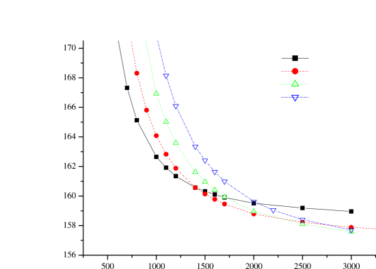
$N$

Figure 1: The ⁴He–⁴He₂ scattering length $\ell_{\rm sc}$ for $l_{\rm max}=0$ in case of the TTY potential as a function of the grid dimension $N\equiv N_{\rho}=N_{\theta}$.

Unlike the trimer binding energies, the ⁴He–⁴He₂ scattering length is much more sensitive to the grid parameters. To investigate this sensitivity, we take increasing values of the cut-off hyperradius $\rho_{\rm max}$, and simultaneously increase the dimension of the grid $N=N_{\theta}=N_{\rho}$. Surely, in such an analysis we can restrict ourselves to $l_{\rm max}=0$. The results obtained for the TTY potential are given in Table 2 and Fig. 1. Inspection of this figure shows that, when increasing the dimension $N$ of the grid, convergence of the ⁴He–⁴He₂ scattering length $\ell_{\rm sc}$ is essentially achieved, however, with different limiting values of $\ell_{\rm sc}$ for different choices of $\rho_{\rm max}$. This concerns, in particular, the transition from $\rho_{\rm max}=600$ Å to $\rho_{\rm max}=700$ Å, while the transition to $800$ Å or even $900$ Å has practically no effect.

Bearing this in mind, we feel justified to choose $\rho_{\rm max}=700$ Å when going over from $l_{\rm max}=0$ to $l_{\rm max}=2$ and 4. The corresponding results are presented in Table 3. There we also show our previous results MSSK where, due to lack of computer facilities, we had to restrict ourselves to $\rho_{\rm max}=460$ Å and $N=605$. We see that an improvement of about 10% is achieved in the present calculations, as indicated already by the trends in Fig. 1.

Table 3 also contains the fairly recent results by Blume and Greene BlumeGreene and Roudnev RoudnevE . The treatment of BlumeGreene is based on a combination of the Monte Carlo method and the hyperspherical adiabatic approach. The one of Ref. RoudnevE employs the three-dimensional Faddeev differential equations in the total angular momentum representation. Our results agree rather well with these alternative calculations.

This gives already a good hint on the quality of our present investigations. A direct confirmation is obtained by extrapolating the curves in Fig. 1. According to this figure, convergence of $\ell_{\rm sc}$ as a function of $N$ is essentially, but not fully, achieved. A certain improvement, thus, is still to be expected when going to higher $N$. In order to estimate this effect we approximate the curves of Fig. 1 by a function of the form

$$\ell_{\rm sc}(N)=\alpha+\frac{\beta}{N-\gamma}.$$ (7)

Clearly, $\ell_{\rm sc}(\infty)=\alpha$. The constants $\alpha$, $\beta$, and $\gamma$ are fixed by the values of $\ell_{\rm sc}$ at $N=1005$, 2005, and $3005$. In this way we get the corresponding optimal scattering lengths $\ell_{\rm sc}(\infty)=157.5$, 156.4, 155.4, and 154.8 Å for $\rho_{\rm max}=600$, 700, 800, and 900 Å, respectively. Comparing with Table 2 shows that the differences between these asymptotic values and the ones for $N=3005$ lie between 1 to 3 Å.

For $l_{\rm max}=4$, $\rho_{\rm max}=700$ Å and the LM2M2 potential the scattering length has been calculated for $N$ = 1005, 1505, and 2005. Employing again the extrapolation formula (7) with $\alpha$, $\beta$, $\gamma$ being chosen according to these values, we find $\ell_{\rm sc}(\infty)$ = 117.0 Å. The difference between the scattering length obtained for $N=2005$ and the extrapolated value, hence, is 1.7 Å. A direct calculation for higher $N$ should lead to a modification rather close to this result. Following this argumentation, we conclude that the true value of $\ell_{\rm sc}$ for the LM2M2 and TTY potentials lies between 115 and 116 Å.

For completeness we mention that besides the above ab initio calculations there are also model calculations, the results of which are given in the last two columns of Table 3. The calculations of Penkov are based on employing a Yamaguchi potential that leads to an easily solvable one-dimensional integral equation in momentum space. The approach of BraatenHammer (see also BHvK and references therein) represents intrinsically a zero-range model with a cut-off introduced to make the resulting one-dimensional Skornyakov-Ter-Martirosian equation STM well defined. The cut-off parameter in BHvK ; BraatenHammer as well as the range parameter of the Yamaguchi potential in Penkov are adjusted to the three-body binding energy obtained in the ab initio calculations. In other words, these approaches are characterized by a remarkable simplicity, but rely essentially on results of the ab initio three-body calculations.

- (1) F. Dalfovo, S. Giorgini, L. P. Pitaevskii, and S. Stringari, Rev. Mod. Phys. 71, 463 (1999).
- (2) T. Köhler, T. Gasenzer, P. S. Julienne, and K. Burnett, Phys. Rev. Lett. 91, 23401 (2003).
- (3) F. Luo, G. C. McBane, G. Kim, C. F. Giese, and W. R. Gentry, J. Chem. Phys. 98, 3564 (1993).
- (4) W. Schöllkopf and J. P. Toennies, Science 266, 1345 (1994).
- (5) R. Grisenti, W. Schöllkopf, J. P. Toennies, G. C. Hegerfeld, T. Köhler, and M.Stoll, Phys. Rev. Lett. 85, 2284 (2000).
- (6) W. Schöllkopf and J. P. Toennies, J. Chem. Phys. 104, 1155 (1996).
- (7) L. W. Bruch, W. Schöllkopf, and J. P. Toennies, J. Chem. Phys. 117, 1544 (2002).
- (8) R. A. Aziz, F. R. W. McCourt, and C. C. K. Wong, Mol. Phys. 61, 1487 (1987).
- (9) R. A. Aziz and M. J. Slaman, J. Chem. Phys. 94, 8047 (1991).
- (10) K. T. Tang, J. P. Toennies, and C. L. Yiu, Phys. Rev. Lett. 74, 1546 (1995).
- (11) A. R. Janzen and R. A. Aziz, J. Chem. Phys. 107, 914 (1997).
- (12) S. Nakaichi-Maeda and T. K. Lim, Phys. Rev. A 28, 692 (1983).
- (13) Th. Cornelius and W. Glöckle, J. Chem. Phys. 85, 3906 (1986).
- (14) J. Carbonell, C. Gignoux, and S. P. Merkuriev, Few–Body Systems 15, 15 (1993).
- (15) B. D. Esry, C. D. Lin, and C. H. Greene, Phys. Rev. A 54, 394 (1996).
- (16) M. Lewerenz, J. Chem. Phys. 106, 4596 (1997).
- (17) E. A. Kolganova, A. K. Motovilov and S. A. Sofianos, Phys. Rev. A. 56, R1686 (1997) (arXiv: physics/9802016).
- (18) A. K. Motovilov, S. A. Sofianos, and E. A. Kolganova, Chem. Phys. Lett. 275, 168 (1997) (arXiv: physics/9709037).
- (19) E. A. Kolganova, A. K. Motovilov, and S. A. Sofianos, J. Phys. B. 31, 1279 (1998) (arXiv: physics/9612012).
- (20) E. Nielsen, D. V. Fedorov, and A. S. Jensen, J. Phys. B 31, 4085 (1998) (arXiv: physics/9806020).
- (21) E. A. Kolganova and A. K. Motovilov, Phys. Atom. Nucl. 62, 1179 (1999) (arXiv: physics/9808027).
- (22) V. Roudnev and S. Yakovlev, Chem. Phys. Lett. 328, 97 (2000).
- (23) D. Blume and C. H. Green, J. Chem. Phys. 112, 8053 (2000).
- (24) A. K. Motovilov, W. Sandhas, S. A. Sofianos, and E. A. Kolganova, Eur. Phys. J. D 13, 33 (2001) (arXiv: physics/9910016).
- (25) P. Barletta, and A. Kievsky, Phys. Rev. A 64, 042514 (2001).
- (26) R. Guardiola, and J. Navarro, Phys. Rev. Lett. 89, 193401 (2002).
- (27) M. T. Yamashita, T. Federico, A. Delfino, and L. Tomio, Phys. Rev. A 66, 052702 (2002).
- (28) V. Roudnev, Chem. Phys. Lett. 367, 95 (2003).
- (29) P. F. Bedaque, H.-W. Hammer, and U. van Kolck, Nucl. Phys. A 646, 444 (1999).
- (30) E. Braatem and H.-W. Hammer, Phys. Rev. A 67, 042706 (2003).
- (31) A. K. Motovilov, Vestnik Leningradskogo Universiteta, 22, 76 (1983) (Russian).
- (32) S. P. Merkuriev and A. K. Motovilov, Lett. Math. Phys. 7, 497 (1983).
- (33) L. D. Faddeev and S. P. Merkuriev, Quantum scattering theory for several particle systems (Kluwer Academic Publishers, Doderecht, 1993).
- (34) S. P. Merkuriev, C. Gignoux, and A. Laverne, Ann. Phys. (N.Y.) 99, 30 (1976).
- (35) F. M. Pen’kov, JETP 97, 536 (2003).
- (36) G. V. Skorniakov and K. A. Ter-Martirosian, Sov. Phys. JETP 4, 648 (1956).