Complex networks of earthquakes and aftershocks

Abstract

We invoke a metric to quantify the correlation between any two earthquakes. This provides a simple and straightforward alternative to using space-time windows to detect aftershock sequences and obviates the need to distinguish main shocks from aftershocks. Directed networks of earthquakes are constructed by placing a link, directed from the past to the future, between pairs of events that are strongly correlated. Each link has a weight giving the relative strength of correlation such that the sum over the incoming links to any node equals unity for aftershocks, or zero if the event had no correlated predecessors. A correlation threshold is set to drastically reduce the size of the data set without losing significant information. Events can be aftershocks of many previous events, and also generate many aftershocks. The probability distribution for the number of incoming and outgoing links are both scale free, and the networks are highly clustered. The Omori law holds for aftershock rates up to a decorrelation time that scales with the magnitude, $m$, of the initiating shock as $t_{\rm cutoff}\sim 10^{\beta m}$ with $\beta\simeq 3/4$. Another scaling law relates distances between earthquakes and their aftershocks to the magnitude of the initiating shock. Our results are inconsistent with the hypothesis of finite aftershock zones. We also find evidence that seismicity is dominantly triggered by small earthquakes. Our approach, using concepts from the modern theory of complex networks, together with a metric to estimate correlations, opens up new avenues of research, as well as new tools to understand seismicity.

I introduction

Seismicity is an exceedingly intermittent phenomena (Kagan, 1994) exhibiting strong correlations in space and time. Since the seismic rate increases sharply after a large earthquake in the region, events typically are classified as aftershocks or main shocks, and the statistics of aftershock sequences are studied. Usually, aftershocks are collected by counting all events within a fixed space-time window  (Gardner and Knopoff, 1974; Keilis-Borok et al., 1980; Knopoff et al., 1982; Knopoff, 2000) following a main event. The size of the window may vary or scale with the magnitude of the main event (Kagan, 2002a), and other refinements have been made (Helmstetter, 2003). However, this method does not allow a likelyhood to be estimated that an event thereby collected is actually correlated to the main event under consideration. As a result, no straightforward algorithm exists to decide if the space-time windows are too large or too small for minimizing errors in the procedure. Also, the method cannot be easily extended to examine remote triggering (Hill et al., 1993; Gomberg et al., 2001) where main shocks may trigger aftershocks at great distance in space, or perhaps far away in time. In addition, aftershocks may have several preceding events to which they are correlated, perhaps with overlapping space-time windows. Using conventional methods the conjecture that aftershocks can rumble on for centuries (Kagan, 2002b) cannot be tested.

In fact, a growing body of work indicates that the distinction between aftershocks and main shocks is relative (Baiesi and Paczuski, 2004; Kagan, 2002b). There is no unique operational way to distinguish between aftershocks and main shocks (Bak et al., 2002). They are not caused by different relaxation mechanisms (Hough and Jones, 1997; Helmstetter and Sornette, 2003). Besides, a strict distinction may not be the most useful way to describe the dynamics of seismicity.

A particular nuisance with employing space-time windows arises from the entanglement of a vast range of scales in space, time and magnitude in seismicity. One scale-free property is the Gutenberg and Richter (1941) (G-R) distribution for the number of earthquakes of magnitude $m$ in a seismic region,

$$P(m)\sim 10^{-b\,m}\quad,$$ (1)

with $b$ usually $\approx 1$. A second is the fractal appearance of earthquake epicenters (Turcotte, 1997; Kagan, 1994; Hirata, 1989), where the fractal dimension $d_{f}\approx 1.6$ in S. California (Corral, 2003). A third is the Omori law (Omori, 1894; Utsu et al., 1995) for the rate of aftershocks in time,

$$\nu(t)\sim\frac{K}{c+t}\quad,$$ (2)

where $c$ and $K$ are constant in time, but depend on the magnitude $m$ (Utsu et al., 1995) of the earthquake.

One way forward has been suggested by (Bak et al., 2002) who take the perspective of statistical physics: Neglecting any classification of earthquakes as main shocks, foreshocks or aftershocks, analyze seismicity patterns irrespective of tectonic features and place all events on the same footing. They consider spatial areas and their subdivision into square cells of length $L$. For each of these cells, only events above a threshold magnitude $m$ are included in the analysis. In this way, one can obtain a distribution of waiting times (Bak et al., 2002; Corral, 2003; Davidsen and Goltz, 2004) and distancesDavidsen and. Paczuski (2004) between successive events with epicenters both in the same cell of linear extent $L$. Since both the threshold magnitude and the length scale of the cell (or the space window) are arbitrary, one looks for robust or universal features of this distribution that appear when these parameters are varied.

We (Baiesi and Paczuski, 2004) have previously introduced an alternative method for characterizing seismicity that completely avoids using fixed space-time windows and, at the same time, makes available powerful concepts and methods that are being developed to describe complex networks (Albert and Barabási, 2002; Bornholdt and Schuster, 2002; Newman, 2003). Here we extend the method to allow more than one incoming link per earthquake. This allows the network to deviate from a tree structure and exhibit characteristic properties of complex networks, such as “clustering” Baiesi (2004), which may be relevant to characterizing seismicity. Our method also takes into account, in an unbiased way, that an aftershock can be correlated to many previous events. By unbiased, we mean that we do not fix any length, time or magnitude scales for identifying aftershocks. Nor do we fix the number of events they can be aftershocks of.

II The Method

A general description of our method is as follows: The first step is to propose, as a null hypothesis (Jaynes, 2003), that earthquakes are uncorrelated in time. Then we detect instances when that hypothesis is strongly violated, indicating that the opposite is true. The second step is to assign a real number, or metric, that quantifies the correlation between any two earthquakes, based on gross violations of the null hypothesis. The third step is to construct a directed network where the events that are correlated according to the metric are nodes connected by links. Each link contains several variables such as the time between the linked events, the spatial distance between their epicenter or hypocenters, the magnitudes of the earthquakes, and the metric or correlation between the linked pairs. We can study the statistical properties of the network and its ensemble of space/time/magnitude variables to gain new insights into seismicity. Note that many variations of the null hypothesis and associated metric are possible, but the key feature of a useful null hypothesis, in this context, is that earthquakes are uncorrelated in time.

The null hypothesis, which we previously used, is that earthquakes occur with a distribution of magnitudes given by the G-R law, with epicenters located on a fractal of dimension $d_{f}$, at random in time. Of course, it is patently false that earthquakes are uncorrelated in time. It is also unclear if epicenters form a monofractal with dimension $d_{f}\leq 2$. The point is to look for strong violations of the null hypothesis.

Consider an earthquake $j$ in the seismic region, which occurs at time $T_{j}$ at location $R_{j}$. Look backward in time to the appearance of earthquake $i$ of magnitude $m_{i}$ at time $T_{i}$, at location $R_{i}$. One can ask, how likely is event $i$ given that event $j$ occurred where and when it did? According to the null hypothesis, the expected number of earthquakes of magnitude within an interval $\Delta m$ of $m_{i}$ that would be expected to have occurred within the time interval $t=T_{j}-T_{i}$ seconds, and within a distance $l=|R_{i}-R_{j}|$ meters is

$$n_{ij}\equiv(\textit{const})\,t\,l^{d_{f}}\,10^{-bm_{i}}\,\Delta m\quad.$$ (3)

Note that the space-time domain $(t,l)$ appearing in Eq. 3 is selected by the particular history of seismic activity in the region and not preordained by any observer. The constant term in Eq. 3 is estimated by the overall seismic rate in the region over the time span of recorded events and is evaluated later. However, our results are insensitive to the precise value of this constant, since its value is absorbed into a threshold we define later, $c_{<}$. We find that many of the statistical properties of the networks are robust with respect to varying parameters such as $c_{<}$, $d_{f}$, and $b$. In particular, we can choose $d_{f}=2$ without substantially varying the results. See also (Baiesi and Paczuski, 2004).

Consider a pair of earthquakes $(i,j)$ where $n_{ij}\ll 1$; so that the expected number of earthquakes according to the null hypothesis is very small. However, event $i$ actually occurred relative to $j$, which, according to the metric, is surprising. Hence, it is unlikely that the pair would occur in that space-time domain if they were uncorrelated. A small value $n_{ij}\ll 1$ indicates that the correlation between $j$ and $i$ is very strong, and vice versa. By this argument, the correlation $c_{ij}$ between any two earthquakes $i$ and $j$ can be estimated to be inversely proportional to $n_{ij}$, or

$$c_{ij}=1/n_{ij}\quad.$$ (4)

As we show later, the distribution of the correlation variables $c_{ij}$ for all pairs ${i,j}$ is extremely broad. Therefore, for each earthquake $j$, some exceptional events in its past have much stronger correlation than all the others combined. These strongly correlated pairs of events can be marked as linked nodes, and the collection of linked nodes forms a sparse network of highly clustered graphs. Unless otherwise stated in this work, earthquakes are linked only if their correlation value, $c_{ij}$, is greater than $c_{<}=10^{4}$, or the expected number of events according to the null hypothesis, $n_{ij}$, is less than $10^{-4}$. The error made in ignoring weakly linked pairs of events is discussed later.

In the language of modern complex network theory (Albert and Barabási, 2002; Bornholdt and Schuster, 2002; Newman, 2003), a time-oriented weighted network grows, where nodes (earthquakes) have internal variables (magnitude, occurrence time, and location), and links between the nodes carry a strength (the correlation $c_{ij}$) and are directed from the older to the newer nodes. Empirically, we find that both the distribution of outgoing and incoming links are scale free. The network is composed of highly clustered, disconnected graphs of correlated earthquakes. Events with incoming links, or aftershocks, typically connect to many previous events rather than just one. However, the networks are sparse and the number of links in the network is much less (about 0.1%) than the number of pairs of earthquakes. We find neither that every earthquake is correlated to every other event, nor that events typically are correlated to zero or one previous events, but a picture in between where the number of events an aftershock is correlated to is scale-free.

Due to the continuous nature of the link variable, $c_{ij}$, no event is purely an aftershock or a main shock, and it is not possible to separate events into distinct classes. This is consistent with previous studies indicating no physical distinction between main shocks and aftershocks (Hough and Jones, 1997; Bak et al., 2002). Note that singularities in Eq. 3 are eliminated by taking a small scale cutoff in time (here $t_{\rm min}=60$ sec) and a minimum spatial resolution (here $l_{\rm min}=100$ meters).

III Data and parameters

The catalog we have analyzed is maintained by the Southern California Earthquake Data Center, and can be downloaded via the Internet at http://www.data.scec.org/ftp/catalogs/SCSN/. We use data ranging from January 1, 1984 to December 31, 2003, and follow a procedure similar to our previous work (see Baiesi and Paczuski (2004) for more details).

Table 1: Network quantities for the Southern California data set, unless otherwise noted.

Quantity	Symbol	Value
magnitude threshold	$m_{<}$	3
magnitude precision	$\Delta m$	0.1
Gutenberg-Richter exponent	$b$	0.95
fractal dimension of epicenters	$d_{f}$	1.6
fractal dimension of hypocenters	$D_{f}$	2.6
number of earthquakes	$N_{\rm node}$	8858

Table 2: Parameters for the network of Southern California obtained with the 2D version of the metric, unless otherwise noted.

Quantity	Symbol	Value
seismicity constant (see Eq. 3)	const	$10^{-11}$
correlation threshold	$c_{<}$	$10^{4}$
number of links	$N_{\rm link}$	166507
average in-degree	$\langle k_{\rm in}\rangle$	$18.8$
number of clusters	$N_{\rm cluster}$	$2252$

Table 3: Parameters for the network of Southern California obtained with the 3D version of the metric, unless otherwise noted.

Quantity	Symbol	Value
seismicity constant (see Eq. 8)	const’	$10^{-15}$
correlation threshold	$c_{<}$	$10^{4}$
number of links	$N_{\rm link}$	$154792$
average in-degree	$\langle k_{\rm in}\rangle$	$17.5$
number of clusters	$N_{\rm cluster}$	$2327$

The relevant quantities for our present work are summarized in Tables 1, 3, and 3. Events with magnitude smaller than $m_{<}=3$ are discarded, and $\Delta m=0.1$. The number of earthquakes or nodes in the network constructed using the entire catalog is $N_{\rm node}=8858$. The $b$-value of the G-R law is $b\simeq 0.95$ for this data set, while $d_{f}\simeq 1.6$ was found by  Corral (2003).

We consider two closely related variants of the metric: in the two-dimensional (2D) version, the earthquake depth is not considered, and the distance between two events $i$ and $j$ is measured as the arc length on the Earth’s surface,

$$l_{ij} =R_{0}\arccos[ \,\sin(\theta_{i})\sin(\theta_{j})+$$ (5)

$$\cos(\theta_{i})\cos(\theta_{j})\cos(\phi_{i}-\phi_{j})\,]\quad,$$

where the Earth radius is $R_{0}=6.3673\times 10^{6}$ meters, and ($\theta_{i}$,$\phi_{i}$) are the latitude and longitude, in radians, of the epicenter of th $i$’th event in the catalogue.

The second version (3D) takes into account the depth $h_{i}$ of each event. Hence Euclidean distances between hypocenters are calculated,

$$l_{ij}=\sqrt{\sum_{a=1}^{3}(x_{i}^{a}-x_{j}^{a})^{2}}$$ (6)

with

$$x_{i}^{1} = (R_{0}-h_{i})\cos\theta_{i}\cos\phi_{i}$$

$$x_{i}^{2} = (R_{0}-h_{i})\cos\theta_{i}\sin\phi_{i}$$ (7)

$$x_{i}^{3} = (R_{0}-h_{i})\sin\theta_{i}$$

and $d_{f}$ in the metric is replaced by the hypocenter fractal dimension $D_{f}$, which is approximated as $D_{f}=d_{f}+1\simeq 2.6$ for Southern California. Thus, the 3D metric is

$$n_{ij}\equiv\textit{const'}\,t\,l^{D_{f}}\Delta m\,10^{-bm_{i}}\quad.$$ (8)

Most of the statistical results we find are not sensitive to the choice of the metric, nor to the precise values of $b$, $d_{f}$, or $D_{f}$. For this reason, we pick as a standard metric the 2D version (Eq. 3), and use the 3D metric only when explicitly stated.

The constant in Eq. 3 was estimated to be $\textit{const}=10^{-11}$ for the 2D metric using the same method as in Baiesi and Paczuski (2004). However in that work a fractal dimension of $d_{f}=1.2$ was inadvertently used to estimate const, resulting in a different value. Similarly, here we compute $\textit{const'}=10^{-15}$ for the 3D metric, Eq. (8). Both values give consistent results, but they are not expected to be precise due to the high variability of seismicity rates in the region even over a time span of years. However, varying the constants, const and const’, in our analysis is equivalent to varying the correlation threshold for linking events, $c_{<}$. We observe that many of the statistical results presented below are robust to variations of $c_{<}$. This is primarily for two reasons. First, as we will show the distribution of link weights $P(c)$ is very broad and doesn’t pick out preferred values. Second, the distributions we compute are weighted using the link weight. Reducing the threshold for included links only adds earthquake pairs that give progressively lower contribution to the final correlation structure. We give later a numerical estimate for the error made in throwing out these degrees of freedom. The advantage, obviously, is that a sparse network with $c_{<}$ chosen appropriatly, enables us to vastly reduce the size of the data set from approximately 10-100 Gigabytes to around 10 Megabytes or so, without losing important information about correlations between earthquakes. The network allows a ’renormalization’ which removes irrelevant degrees of freedom, or links with low weights $c_{ij}$ while keeping important ones.

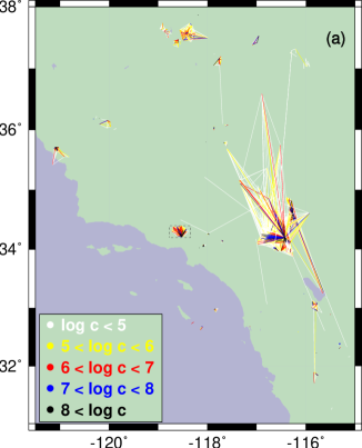
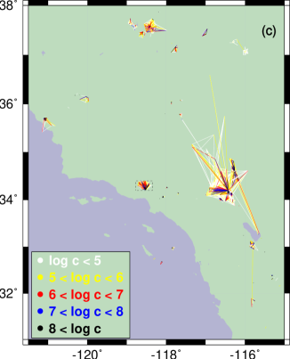
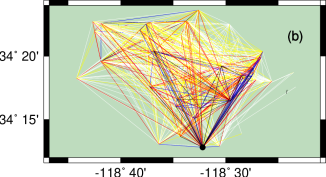
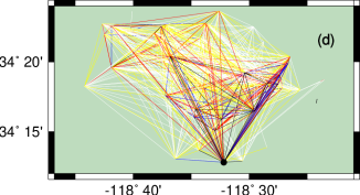
Figure 1: (a) Scale free network of earthquakes obtained with the 2D metric using $m_{<}=4$ and $c_{<}=10^{4}$. This network has $791$ nodes, and its $7931$ links follow the color code in the legend. Several clusters are evident, the biggest being related to the Landers earthquake. The Northridge cluster, enclosed within a dashed box in (a), is enlarged in (b), where the solid black dot represents the epicenter of the Northridge event. Figures (c) and (d) are obtained using the 3D metric with $m_{<}=4$ and $c_{<}=5\times 10^{3}$ giving $7947$ links, very close to the number of links in the 2D version. Note that the networks found using these two metrics are similar, indicating that the method is robust to variations in the metric.

IV Results

Networks constructed using our method are shown in Fig. 1. For comparison, networks obtained with the 2D metric [Fig. 1(a) and (b)] and with the 3D metric [Fig. 1(c) and (d)] are both displayed. For visual clarity, a higher threshold for earthquake magnitudes $m_{<}=4$ was used in order to reduce the number of nodes and links in the figure. Adjusting the parameter $c_{<}$ slightly, two networks with a similar number of links, with very similar clusters of correlated events are formed. There is a more abundant presence of long distance links in the 2D version but the similar details in the Northridge clusters [Fig. 1(b) and (d)] suggest that it is mainly seismic history that determines the network structure, rather than the precise details of our metric.

IV.1 Explanation of Method

Fig. 2 shows the probability distribution of correlation values, $P(c)$, obtained by sampling the values $c_{ij}$ over all earthquake pairs in the data set. It is a fantastically broad distribution that exhibits power law behavior over sixteen orders of magnitude (in the 3D case):

$$P(c)\sim c^{-\tau}$$ (9)

with $\tau=1.43\pm 0.03$ using the 2D metric and $\tau=1.38\pm 0.03$ using the 3D one.

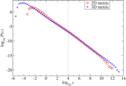
Figure 2: The probability distribution of the correlation, $c$, between all earthquake pairs in the data base, with $m_{<}=3$, using both the 2D metric and the 3D one. They are scale free distributions over many orders of magnitude. The threshold $c_{<}=10^{4}$ where correlations are considered significant and links are made is indicated in the figure. Note that, with that threshold, most links are eliminated from the network, giving a reduced data set to examine seismic properties.

Given such a broad distribution, for any earthquake $j$, some extreme events $i$ exist whose correlation $c_{ij}$ are much larger than all the others. Therefore, it makes sense to represent these earthquake pairs as nodes that are linked, while not linking pairs that have much smaller values of $c_{ij}$. Then the sequence of earthquakes may be usefully represented as a sparse network, where links exist between the most strongly correlated events, i.e. those pairs $(i,j)$ where $c_{ij}>c_{<}$. Hence a natural decomposition of the network into disconnected clusters is achieved, where the first earthquake in the directed cluster has no incoming link, or correlation variable into it greater than $c_{<}$. Clearly, the first earthquake in the entire catalogue also no incoming link. The correlated events are reliably detected when $c_{<}$ is greater than one but not extremely large. In the latter case, correlated events detach, and a very fragmented network appears. For small $c_{<}$ some uncorrelated events make links, and a giant cluster appears. Both for the 2D and for the 3D case we set $c_{<}=10^{4}$, unless otherwise noted, obtaining a similar number of links in the realization of the networks.

IV.2 The Scale-Free Network

The resulting network of earthquakes is scale free. As shown in Fig. 3, both the distribution of the number of incoming links, or the “in-degree” $k_{\rm in}$, to a node and the distribution of the number of outgoing links, or the “out-degree” $k_{\rm out}$, to any node exhibit power law behavior,

$$P(k_{\rm in})\sim 1/k_{\rm in}\,,\quad P(k_{\rm out})\sim 1/k_{\rm out}$$ (10)

up to a degree $\approx 100$.

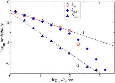
Figure 3: The in-degree and out-degree distributions of the network of earthquakes and aftershocks. The out-degree, $k_{\rm out}$, is the number of outgoing links from an earthquake, linking it to its aftershocks. The in-degree, $k_{\rm in}$, is the number of incoming links to an earthquake, linking it to its main shocks. These two distributions are similar. Also shown is the distribution of the weighted number of aftershocks, $P(N_{{\rm after}})$, from any event, using $\eta=1$ in Eqs. 11 and  12. This has the same scaling behavior as the extremal network, with $\eta\rightarrow\infty$.

IV.2.1 Aftershocks with more than one main shock

Since an earthquake can have more than one incoming link, in attributing aftershocks to an event we must be careful not to overweight aftershocks with many incoming links. To prevent the overcounting of aftershocks, one can consider a new event with two incoming links, for example, to be “half an aftershock” of both of its precursors, or they can be weighted in a different fashion according to their correlation values. In general, we can attribute the relative correlation to previous events, so that each event contributes a total weight of unity to the global aftershock number if it is linked to at least one previous event, and zero otherwise, as follows:

For each event $j$ that has at least one incoming link, so that it can be called an aftershock, define a weight for each ”parent” earthquake $i$ it is linked to as

$$w_{ij}={c_{ij}^{\eta}\over\sum_{k}^{\rm in}c_{kj}^{\eta}}\quad,$$ (11)

where the sum is over all earthquakes $k$ with links going into $j$. The weighted number of aftershocks attributable any event $i$ is then

$$N_{{\rm after},i}=\sum_{j}^{\rm out}w_{ij}\quad.$$ (12)

Here, the sum is over all of the outgoing links from event $i$. In the limit that $\eta\rightarrow\infty$, the extremal network studied by Baiesi and Paczuski (2004) is recovered, since only the single incoming link to aftershock $j$, with the largest correlation $c_{ij}$, contributes. In that case, for each node, the quantity $N_{{\rm after}}$ discussed here coincides with the quantity $k_{\rm out}$ in Baiesi and Paczuski (2004). In the following, we consider the case $\eta=1$.

Sampling over all earthquakes, we get a probability distribution for the number of (weighted) aftershocks as also shown in Fig. 3. It is a power law distribution, $P(N_{\rm after})\sim(N_{\rm after})^{-\gamma}$ scaling over more than three decades, with an index $\gamma=2.0(1)$. This distribution is very close to the distribution we obtained previously for the number of aftershocks in the extremal network, corresponding to the limit $\eta\rightarrow\infty$. The distribution for the number of weighted aftershocks appears to be universal, in the sense that the power law exponent does not depend on $\eta$, for $\eta\geq 1$. Note that chosing a positive $\eta$ gives more weight to more strongly correlated pairs and is therefore consistent with using a threshold $c_{<}$ to eliminate weakly correlated ones.

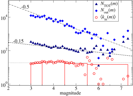
Figure 4: The total number of outgoing links from all events of magnitude $m$ (diamonds), the total number of weighted aftershocks of all events of magnitude $m$ (triangles) and average number of incoming links ($\langle k_{\rm in}(m)\rangle$, circles and histogram) as a function of $m$. The first two quantities have a scaling consistent with the law $\sim 10^{\alpha m}$, with $\alpha^{\prime}\approx b-0.5\approx 0.45$ for outgoing links, and $\alpha\approx b-0.15\approx 0.8$ for weighted aftershocks. For $\langle k_{\rm in}(m)\rangle$ there is no evident departure from the average value $\langle k_{\rm in}\rangle\simeq 18.8$ (dotted line).

IV.2.2 Is Seismicity driven by small or large earthquakes?

The average number of aftershocks of an earthquake of magnitude $m$ has been proposed to scale with $m$ (Utsu, 1969; Kagan and Knopoff, 1987) as

$$N_{\rm after}(m)\sim 10^{\alpha m}\quad.$$ (13)

Larger main shocks release more energy and therefore “trigger” more aftershocks than smaller earthquakes. However, smaller earthquakes are more frequent, as indicated by the G-R relation. The total number of aftershocks generated by all earthquakes of magnitude $m$ is therefore given by the product of these two relations as

$$N_{\rm TOT}(m)=N_{\rm after}(m)P(m)\sim 10^{(\alpha-b)m}\quad.$$ (14)

If the exponent $\alpha>b$ then small earthquakes are the dominant triggering mechanism for seismicity, whereas if $\alpha<b$ the large earthquakes dominate aftershock production. Often it is assumed that $\alpha=b$ (Kagan and Knopoff, 1987; Reasenberg and Jones, 1989).

Recently, Helmstetter (2003) analyzed earthquake catalogues by means of a ”stacking” method using space-time windows, and found that aftershocks were predominantly triggered by small earthquakes. She determined the value of the exponent $\alpha$ to be between $\alpha=0.72$ and $\alpha=0.82$, depending on the parameters of the aftershock detection algorithm that she used.

Fig. 4 shows $N_{\rm TOT}(m)$ obtained using the 2D metric with $\eta=1$. The results shown in this figure also suggests that small earthquakes are the dominant mechanism driving aftershock production. We determine the value of the exponent $\alpha\approx 0.8$, consistent with Helmstetter’s previous findings. Thus at this rather detailed level, results obtained using our method are consistent with results obtained using traditional methods of aftershock detection. This is true despite the fact that aftershocks in our algorithm are typically attached to many previous events rather than just one, and no space-time scales are used by us for aftershock identification.

Fig. 4 also shows the total number of links emanating from events of magnitude $m$, $N_{\rm out}(m)$. This corresponds to an unweighted aftershock number, with $N_{\rm out}(m)\sim 10^{-(\alpha^{\prime}-b)}$ and $\alpha^{\prime}=0.45$. Since both $\alpha$ and $\alpha^{\prime}$ are less than $b$, our results suggest that irrespective of the manner in which aftershocks are weighted, small earthquakes are the dominant mechanism driving aftershock production. Note however, that the largest events may appear to present a deviation from this behavior, but the statistical uncertainties of single events are large.

IV.2.3 Båth’s Law

In Fig. 4, we also show the dependence of the number of incoming links to a node on its magnitude. The quantity $\langle k_{\rm in}(m)\rangle$, is the average number of incoming links to earthquakes of magnitude $m$. This quantity is independent of earthquake magnitude for $3\leq m\leq 5$. For larger magnitudes, the poor statistics forces us to average $k_{\rm in}(m)$ over wider bins, chosen so that there is a significant number of events inside each one. These averages are indicated as horizontal lines in Fig. 4, while vertical lines denote the bin boundaries. The averages do not show any detectable trend for larger earthquakes.

Our results suggest that earthquakes of all magnitudes are equally likely to be aftershocks, and support the conclusion reached by Helmstetter and Sornette (2003) that observations of Båth’s law are due to biases in labelling earthquakes as aftershocks. According to Båth’s law (Båth, 1965), the average magnitude difference between a main shock and its largest aftershock is around 1.2, independently of the main shock magnitude. Of course, the definitions we use here for main shocks, as nodes giving outgoing links, and aftershocks, where nodes have incoming links (so that a single event can be both a main shock and aftershock), differs from the standard definition.

IV.2.4 Clustering of nodes

Among the concepts in network theory that may be useful to characterize seismicity, and are not accessible via other approaches, the clustering of nodes deserves particular attention. Indeed, the clustering in space and time of earthquakes can be quantified in their network by the clustering coefficient. The clustering coefficient of a node $i$ is the number $\Delta_{i}$ of linked triangles it forms with its $k_{i}$ neighbors (or equivalently, the pairs of linked neighbors) divided by the maximum number of linked triangles it could potentially have ($k_{i}(k_{i}-1)/2$), i.e.,

$$C_{i}=\frac{2\Delta_{i}}{k_{i}(k_{i}-1)}\quad.$$ (15)

This definition ignores the directionality of links. Thus, in this formula the degree of node $i$, is the sum of its incoming and outgoing degrees, i.e. $k_{i}=k_{i,\rm in}+k_{i,\rm out}$. In all cases $0\leq C_{i}\leq 1$, and $C_{i}=0$ if less than two links are joined to node $i$, or if no links between its linked neighbors are present, while $C_{i}=1$ only if all neighbors are linked to each other.

Using Eq. (15) to compute the average clustering coefficient of the network,

$$C=\frac{1}{N_{\rm node}}\sum_{i=1}^{N_{\rm node}}C_{i}\quad,$$ (16)

we obtain $C=0.50$ for $m_{<}=3$. This value is relatively stable with respect to variations of $m_{<}$. For instance, with $m_{<}=4.5$ we get $C=0.55$. The same values are obtained for the 3D version of the metric. These are remarkably high values of $C$, compared to many other complex networks, such as technological or biological ones (Newman, 2003).

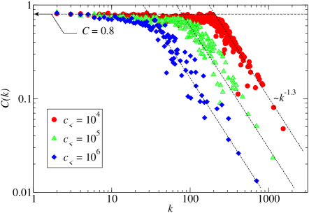
Figure 5: The network density, or clustering coefficient as a function of the degree, $k$, of a node, where $k=k_{in}+k_{out}$. For small values of $k$, the clustering coefficient is independent of $k$ and $c_{<}$, and $C\approx 0.80$. For large values of $k$, $C(k)$ tends toward power law behavior $C(k)\sim k^{-\delta}$, with $\delta\approx 1.3$. The power law regime takes place at smaller $k$ for larger thresholds $c_{<}$.

Universal clustering properties of seismic networks

The average of the clustering coefficient can be performed over nodes with the same degree $k$. This quantity is shown in Fig. 5, where one can observe that it does not depend on $k$ for small values of $k$ and approaches a power law $C(k)\sim k^{-\delta}$ with $\delta\approx 1.3$ for large values of $k$. This power law behavior is typically found in networks with a modular structure (Ravasz and Barabási, 2003). At small $k$, $C(k)$ approaches a universal value approximately equal to $0.8$, which is independent of $k$ and of the thresholds $c_{<}$ and $m_{<}$ used to construct the network. The power law exponent $\delta$ at large values of $k$ also appears to be independent of $c_{<}$, and may also be a universal quantity for seismic networks.

IV.3 Scaling Law for Aftershock Distances

In the network constructed using the 2D metric, the link length, $l$, is the distance between the epicenters of an earthquake and one of its aftershocks, weighted according to the link weight $w$. In the corresponding network constructed using the 3D metric, the link length is the distance between the hypocenters of an earthquake and one of its aftershocks, weighted according to the link weight $w$. The distribution $P_{m}(l)$ of link lengths depends on the magnitude $m$ of the predecessor, being on average greater for larger $m$. To compute this distribution, we put the weight of each link into a bin corresponding to its $l$ value and the magnitude of the predecessor $m$ to get $P_{m}(l)$. A maximum in the distribution occurs, which shifts to larger $l$ on increasing $m$, as shown in Fig. 6. This behavior is superficially consistent with using larger space-time windows to collect aftershocks from larger events, or the Kagan (2002a) hypothesis of aftershock zone scaling with main shock magnitude.

IV.3.1 Comparison with Aftershock Zone Scaling

It is widely believed that an aftershock zone exists which is equivalent to the rupture length. Within the aftershock zone, earthquakes generate aftershocks, while outside the zone they do not. The rupture length, $R$, is believed to scale as $R\sim 10^{0.5m}$ with the magnitude of the main shock. This is a restatement of the relation derived by Kanamori and Anderson (1975), who argued that the seismic moment $M\sim 10^{1.5m}$ scales with $R$ as $M\sim R^{3}$, at least for intermediate magnitude earthquakes. For a generalization to all earthquakes, see Kagan (2002a). In this scenario main shocks of all magnitudes generate aftershocks at the same rate within their respective aftershock zones, so that the greater number of aftershocks coming from large events is due solely to their larger aftershock zones. Needless to say, the observation of aftershock zone scaling is based on the idea that the aftershock zone is finite – on the order of tens of kilometers for large main shocks.

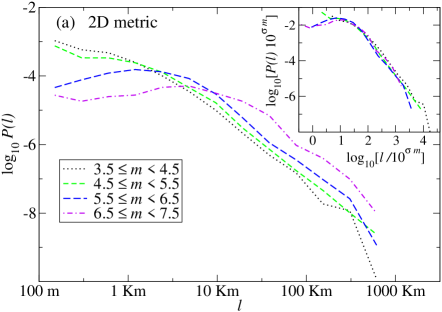
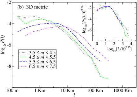
Figure 6: Link length distribution for different magnitudes of the emitting earthquake, (a) for the 2D case and (b) for the 3D one. The length where the maximum in the distribution occurs increases with magnitude roughly as $l_{\rm max}\sim 10^{0.37m}$ in both cases. Both distributions also have a fat tail, extending up to hundreds of kilometers even for intermediate magnitude events. These distributions are consistent with a hierarchical organization of events, where big earthquakes preferentially link at long distance with intermediate ones, which in turn link to more localized aftershocks, and so on. Insets: Distributions rescaled according to Eq. 17 with $\sigma=0.37$ and with $m$ equal to the central magnitude of the range for each distribution.

In contrast, we find the distribution of lengths between main shocks and their aftershocks exhibits no cutoff at large distances, but rather decays slowly as a power law with $l$, up to the linear extent of the seismic region covered by the catalog, hundreds of kilometers. The two distributions are both consistent with a scaling ansatz:

$$P_{m}(l)\simeq 10^{-\sigma m}F\big{(}l/10^{\sigma m}\big{)}\,$$ (17)

where $l$ is measured in meters and $F(x)$ is a scaling function. Remarkably in both cases, $\sigma\approx 0.37$. Note in particular that $\sigma\neq 0.5$.

For $x\gg 1$, the tail of the scaling function is a power law, i.e. $F(x)\sim x^{-\lambda}$ with $\lambda\approx 2$ (2D) or $\lambda\approx 2.6$ (3D). The results obtained using the data collapse technique applied using ansatz (17) are shown in the insets of Fig. 6(a) and (b). Such slow decays at large distances calls into question the use of sharply defined space windows for collecting aftershocks, as already pointed out by Ogata (1998a). The length scale we find $l_{m}^{*}\sim 10^{0.37m}$ to describe the fat-tailed distribution of distances between earthquakes and their aftershocks should not be confused with the scaling of a finite aftershock zone as proposed by Kagan (2002a). Instead, our results are consistent with observations of remote triggering of aftershocks by Hill et al. (1993) and Gomberg et al. (2001) as well as the observation that the distribution of distances between subsequent earthquakes in regions of size $L$ is a power law, not trivially given by the correlation dimension, $d_{2}$ of earthquakes, and which is cutoff only by the size of the region $L$ Davidsen and. Paczuski (2004).

IV.4 The Omori Law for Earthquakes of All Magnitudes

Figure 7 shows the rate of aftershocks for the Landers, Hector Mine, and Northridge events, obtained with the 2D metric. The weights, $w$, of the links to aftershocks occurring at time $t$ after one of these events are binned into geometrically increasing time intervals. The number of weighted aftershocks in each bin is then divided by the temporal width of the bin to obtain a rate of weighted aftershocks per second. The same procedure is applied to each remaining event, not aftershocks of these three. An average is made for the rate of aftershocks linked to events having a magnitude within an interval $\Delta m$ of $m$. Figure 7 also shows the averaged results for $m=3$ (1871 events), $m=4$ (175 events), $m=5$ (28 events) and $m=5.9$ (4 events).

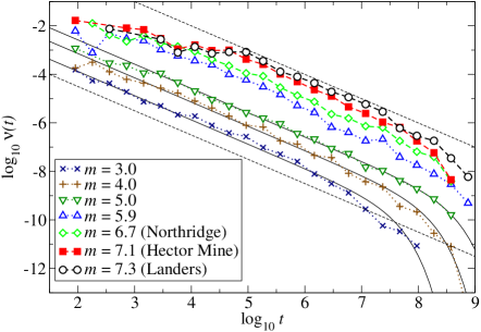
Figure 7: The Omori law for aftershock rates. These rates are measured for aftershocks linked to earthquakes of different magnitudes. For each magnitude, the rate is consistent with the original Omori law, Eq. 2, up to a cutoff time that depends on $m$. As guides to the eye, dashed lines represent a decay $\sim 1/t$. The dense curves represent the fits obtained by means of Eq. 19 for $m=3$, $m=4$, and $m=5$.

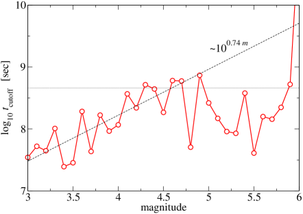
Figure 8: Decorrelation time, $t_{\rm cutoff}$ of the aftershock rates to fall out of the Omori regime, as a function of the earthquake magnitude. The horizontal line indicates 20 years, i.e. the time span of the catalogue. The dashed line is the interpolation given in Eq. 20.

The collection of aftershocks linked to earthquakes of all magnitudes is one of the main results of our method. Even intermediate magnitude events can have aftershocks that persist up to years. Earthquakes of all magnitudes have aftershocks which decay according to the Omori law (Omori, 1894; Utsu et al., 1995),

$$\nu(t)\sim\frac{K}{c+t}\quad,\quad{\rm for}\ t<t_{\rm cutoff}$$ (18)

where $c$ and $K$ are constant in time, but depend on the magnitude $m$ (Utsu et al., 1995) of the earthquake. We find that the Omori law persists up to a decorrelation time $t_{\rm cutoff}$ that also depends on $m$.

A rough estimate of the decorrelation times can be extracted by non-linear fits of $\log_{10}\nu_{m}(t)$ vs $\log_{10}t$, using an interpolating function

$$\nu_{m}(t)\sim t^{-1}e^{-t/t_{\rm cutoff}}\quad.$$ (19)

The range of the fit excludes short times, where the the aftershock rates are not yet scaling as $1/t$. The short time deviation from power law behavior is presumably due to saturation of the detection system, which is unable to reliably detect events happening at a fast rate. However, this problem does not occur at later times, where the rates are lower. Some examples of these fits are also shown in Fig. 7 for the intermediate magnitude events.

In Fig. 8 we show the resulting values of $t_{\rm cutoff}$, for $m$ up to $6$. The horizontal dotted line represents the time span of the catalogue we study, which precludes accurate estimates of much longer $t_{\rm cutoff}$. Thus, from the rates of aftershocks of events with $3\leq m\leq 4.6$, where the time span of the catalogue is comparable or longer than the estimated decorrelation time, we find that the increase of $t_{\rm cutoff}$ with $m$ can be fitted by the function

$$t_{\rm cutoff}(m)\simeq 10^{5.25+0.74m}\quad{\rm sec}\quad,$$ (20)

represented as a dashed line in Fig. 8. It roughly corresponds to $t_{\rm cutoff}\approx 11$ months for $m=3$, and to $t_{\rm cutoff}\approx 5$ years for $m=4$. An extrapolation yields $t_{\rm cutoff}\approx 1400$ years for an event with $m=7.3$ such as the Landers event! However, we stress that Eq. 20 is just rough estimate of $t_{\rm cutoff}(m)$.

Note that Helmstetter (2003) also found an Omori law for aftershocks of earthquakes of all magnitudes using finite space-time windows. However, for this reason, she was not able to estimate the decorrelation of aftershocks or the cutoff in the duration of the Omori regime for different magnitudes.

V Discussion

At present, we are unaware of any reliable method to determine the best metric. Thus, the best route to study how sensitive the results are to variations of the metric or to the parameters of the metric. Although we have not yet made an exhaustive and detailed study to determine which properties may be universal and hold for many different metrics, several general conclusions are already apparent.

V.1 Robustness with respect to changes in parameters

Many of the statistical results we find are relatively robust with respect to variations in the metric. For instance, using both the 2D metric (Eq. 3) and the 3D metric (Eq. 8), similar networks are found as indicated qualitatively in Fig. 1. In addition, the scaling behaviors demonstrated in Figs. 2-7 are independent of the metric, with the notable exception of the exponent $\lambda$ characterizing the fat tailed distribution of aftershock distances. However, the exponent $\sigma$ for the rescaled variable combining main shock magnitude and aftershock distance is independent of the metric, as is the Omori behavior. Furthermore, the distribution of correlations $P(c)$ depends only weakly on the metric, and the scale-free and clustering properties of the network are insensitive as well.

One could object that the values of $b$, $d_{f}$ and $D_{f}$ can depend on the region of the Earth being considered, or may fluctuate depending on the specific fault zone being studied. However, the statistical results we find, as shown in the Figures, are also robust to variations in either of these parameters, or of the threshold $m_{<}$. This robustness was also found in the Baiesi and Paczuski (2004) studies of the extremal earthquake network. For instance, varying $d_{f}$ over a wide range, from $1$ to $2$ does not alter considerably the distribution of incoming or outgoing links. The distribution of correlations $P(c)$, is even more insensitive to variations of $b$ and $d_{f}$. Also the Omori law with $p\approx 1$, shown in Fig. 7, does not depend sensibly on the parameters, and holds for aftershocks linked to earthquakes of all magnitudes.

Our interpretation of this observed robustness is that the correlation structure of seismicity is unambiguous and clear-cut, and has a network structure similar to other complex networks. Even if we use an approximate measure, or metric, the underlying correlations are sufficiently strong that they survive the approximation and can be reliably detected.

V.2 Errors and Data Set Reduction

One could also object that the parameter $c_{<}$ is arbitrary, and its choice plays a similar role to choosing space-time windows in the traditional manner. However, one can consider all pairs of earthquakes, using their weights $c_{ij}$, so the parameter $c_{<}$ is conceptually unnecessary. This differs from the necessity of choosing space-time windows in the traditional approach. However, as a practical matter, to reduce the size of the data set, it is useful to choose a particular $c_{<}$, and thereby construct a sparse network. The choice involves a trade-off between the amount of data stored, and the accuracy of the representation of seismicity one can make using that data set. From the distribution $P(c)$ shown in Fig. 2, and from the average number of incoming links $\langle k_{in}\rangle$ with a given choice of $c_{<}$, we can estimate the error made in throwing out weak links. The average correlation $c$ contribution from all of the $\approx N_{\rm node}=8858$ incoming links that are pruned from any earthquake when imposing the threshold $c_{<}$ is

$$N_{\rm node}\int_{c_{min}}^{c_{<}}cP(c)dc\simeq AN_{\rm node}c_{<}^{2-\tau}\quad,$$ (21)

where $A$ is a constant given by the amplitude of $P(c)$, and $c_{min}$ is the minimum value of $c$ observed in the measurement of $P(c)$.

The average correlation contribution from the incoming links actually represented in the network with that choice of $c_{<}$ is

$$\langle k_{in}\rangle\int_{c_{<}}^{c_{max}}cP(c)dc\simeq A\langle k_{in}\rangle c_{max}^{2-\tau}\quad,$$ (22)

with $c_{max}\approx 10^{12}$ for the 2D metric. The relative error with a given $c_{<}$ can thus be estimated as

$${\rm Error}=\frac{N_{\rm node}}{\langle k_{in}\rangle}\big{(}\frac{c_{<}}{c_{max}}\big{)}^{2-\tau}\quad.$$ (23)

With our choice $c_{<}=10^{4}$ we get an estimate of the relative error to be approximately one percent, or ${\rm Error}=0.013$ with the fraction the data set stored $N_{links}/N_{\rm node}^{2}\approx 0.002$. In other words, throwing out about $99.8\%$ of the data set we can accurately represent the correlation structure of seismicity using a sparse network with an estimated error of order one percent. Conversely, we are not aware of any quantitative estimate of the error with particular choices of space time windows.

V.3 Bench mark test for models of seismicity

The statistical properties of the network of seismicity we find can be used to test various models of seismicity. A self-organized critical model proposed by Olami et al. (1992) exhibits a universal Gutenberg-Richter law for earthquakes (Lise and Paczuski, 2001), independent of the dissipation parameter, as well as foreshocks and aftershocks (Hergarten and Neugebauer, 2002). However, no evident self-organized spatial structure corresponding to the recurrence of earthquakes on a heterogeneous system of faults exists. For this reason, we believe it is unlikely that this model can reproduce the observed network properties of seismicity. Although no satisfactory dynamical model of the self-organization of the Earth’s crust and resultant seismicity exists at present, a stochastic branching process, known as the ETAS model (Kagan and Knopoff, 1987; Ogata, 1998a), or its spatially extended version (Helmstetter and Sornette, 2002) could be tested by constructing a network using our method for particular realizations of that process in space, time and magnitude, and comparing with our results. For instance, the appearance of the scaling variable $l10^{-\sigma m}$ combining spatial distances with main shock magnitude could be ascertained. Since the distance variable between mother daughter pairs in the spatially extended ETAS model is chosen from a power law distribution, $\Phi(\vec{r})$, independent of the parent’s magnitude, this model is unlikely to reproduce observed behavior and would have to be modified. Conversely, one could also check if our method of constructing networks linking main shocks and aftershocks correctly identifies mother-daughter pairs given by the algorithm of the ETAS process or if there might be differences.