Enhanced transmission versus localization of a light pulse
by a subwavelength metal slit

Abstract

The existence of resonant enhanced transmission and collimation of light waves by subwavelength slits in metal films [for example, see T.W. Ebbesen et al., Nature (London) 391, 667 (1998) and H.J. Lezec et al., Science, 297, 820 (2002)] leads to the basic question: Can a light pulse be enhanced and simultaneously localized in space and time by a subwavelength slit? To address this question, the spatial distribution of the energy flux of an ultrashort (femtosecond) wave-packet diffracted by a subwavelength (nanometer-size) slit was analyzed by using the conventional approach based on the Neerhoff and Mur solution of Maxwell’s equations. The results show that a light pulse can be enhanced by orders of magnitude and simultaneously localized in the near-field diffraction zone at the nm- and fs-scales. Possible applications in nanophotonics are discussed.

I Introduction

In the last decade nanostructured optical elements based on scattering of light waves by subwavelength-size metal objects, such as particles and screen holes, have been investigated intensively. The most impressive features of the optical elements are resonant enhancement and spatial localization of optical fields by the excitation of electron waves in the metal (for example, see the studies Neer ; Harr ; Betz1 ; Ash ; Lewi ; Betz2 ; Pohl ; Ebbe ; Leze ; Port ; Hibb ; Gar1 ; Gar2 ; Dog ; Li ; Stoc ; Kuk1 ; Kuk2 ; Stav ; Bori ; Taka ; Yang ; Cschr ; Trea ; Salo ; Cao ; Smol ; Barb ; Alte ; Dykh ; Stee ; Nawe ; Sun ; Shi ; Scho ; Naha ; Gome ). Recently some nanostructures, namely a single subwavelength slit, a grating with subwavevelength slits, and a subwavelength slit surrounded by parallel deep and narrow grooves attracted a particular attention of researchers. The study of resonant enhanced transmission and collimation of waves in close proximity to a single subwavelength slit acting as a microscope probe Neer ; Harr ; Betz1 was connected with developing near-field scanning microwave and optical microscopes with subwavelength resolution Ash ; Lewi ; Betz2 ; Pohl . The resonant transmission of light by a grating with subwavelength slits or a subwavelength slit surrounded by grooves is an important effect for nanophotonics Ebbe ; Leze ; Port ; Hibb . The transmissivity, on the resonance, can be orders of magnitude greater than out of the resonance. It was understood that the enhancement effect has a two-fold origin: First, the field increases due to a pure geometrical reason, the coupling of incident plane waves with waveguide mode resonances located in the slit, and further enhancement arises due to excitation of coupled surface plasmon polaritons localized on both surfaces of the slit (grating) Port ; Hibb ; Gar1 . A dominant mechanism responsible for the extraordinary transmission is the resonant excitation of the waveguide mode in the slit giving a Fabry-Perot like behaviour Hibb . In addition to the extraordinary transmission, a series of parallel grooves surrounding a nanometer-size slit can produce a micrometer-size beam that spreads to an angle of only few degrees Leze . The light collimation, in this case, is achieved by the excitation of coupled surface plasmon polaritons in the grooves Gar1 . At appropriate conditions, a single subwavelength slit flanked by a finite array of grooves can act as a ”lens” focusing light Gar2 . It should be noted that the diffractive spreading of a beam can be reduced also by using a structured aperture or an effective nanolens formed by self-similar linear chain of metal nanospheres Dog ; Li .

New aspects of the problem of resonantly enhanced transmission and collimation of light are revealed when the nanostructures are illuminated by an ultra-short (femtosecond) light pulse Stoc ; Kuk1 ; Kuk2 ; Stav ; Bori . For instance, in the study  Stoc , the unique possibility of concentrating the energy of an ultrafast excitation of an ”engineered” or a random nanosystem in a small part of the whole system by means of phase modulation of the exciting fs-pulse was predicted. The study  Kuk1 theoretically demonstrated the feasibility of nm-scale localization and distortion-free transmission of fs visible pulses by a single metal slit, and further suggested the feasibility of simultaneous super resolution in space and time of the near-field scanning optical microscopy (NSOM). The quasi-diffraction-free optics based on transmission of pulses by a subwavelength nano-slit has been suggested to extend the operation principle of a 2D NSOM to the ”not-too-distant” field regime (up to $\sim$ 0.5 wavelength) Kuk2 . Some interesting effects, namely the pulse delay and long living resonant excitations of electromagnetic fields in the resonant-transition gratings were recently described in the studies Stav ; Bori .

The great interest to resonant enhanced transmission, spatial localization (collimation) of continuous waves and light pulses by subwavelength metal slits leads to the basic question: Can a light pulse be enhanced and simultaneously localized in space and time by a subwavelength slit? If the field enhancement can be achieved together with nm-scale spatial and fs-scale temporal localizations, this could greatly increase the potentials of the nanoslit systems in high-resolution applications, especially in near-field scanning microscopy and spectroscopy. In the present article we test whether the resonant enhancement could only be obtained at the expense of the spatial and temporal broadening of a light wavepacket. To address this question, the spatial distribution of the energy flux of an ultrashort (fs) pulse diffracted by a subwavelength (nanosized) slit in a thick metal film of perfect conductivity will be analyzed by using the conventional approach based on the Neerhoff and Mur solution of Maxwell’s equations. In short, we first will summarize the theoretical development of Neerhoff and Mur (Section II) and the model will then be used to calculate the spatial distribution of the energy flux of the transmitted pulse (wavepacket) under various regimes of the near-field diffraction (Section III). We will show that a light pulse can be enhanced by orders of magnitude and simultaneously localized in the near-field diffraction zone at the nm- and fs-scales. The implications of the results for diffraction-unlimited near- and far-field optics will then be discussed. In Section IV we summarize the results and present the conclusions.

II Theoretical background

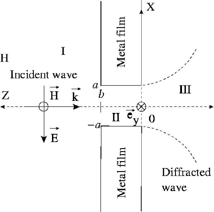
Figure 1: Propagation of a continuous wave through a subwavelength nano-sized slit in a thick metal film.

An adequate description of the transmission of light through a subwavelength nano-sized slit in a thick metal film requires solution of Maxwell’s equations with complicated boundary conditions. The light-slit interaction problem even for a continuous wave can be solved only by extended two-dimensional $(x,z)$ numerical computations. The three-dimensional $(x,z,t)$ character of the pulse-slit interaction makes the numerical analysis even more difficult. Let us consider the near-field diffraction of an ultrashort pulse (wave-packet) by a subwavelength slit in a thick metal screen of perfect conductivity by using the conventional approach based on the Neerhoff and Mur solution of Maxwell’s equations. Before presenting a treatment of the problem for a wave-packet, we briefly describe the Neerhoff and Mur formulation Neer ; Betz1 for a continuous wave (a Fourier $\omega$-component of a wavepacket). The transmission of a plane continuous wave through a slit (waveguide) of width $2a$ in a screen of thickness $b$ is considered. The perfectly conducting nonmagnetic screen placed in vacuum is illuminated by a normally incident plane wave under TM polarization (magnetic-field vector parallel to the slit), as shown in Fig. 1. The magnetic field of the wave is assumed to be time harmonic and constant in the $y$ direction:

$${\vec{H}}(x,y,z,t)=U(x,z){\exp}(-i\omega{t}){\vec{e}}_{y}.$$ (1)

The electric field of the wave (1) is found from the scalar field $U(x,z)$ using Maxwell’s equations:

$${E_{x}}(x,z,t)=-{\frac{ic}{\omega{\epsilon_{1}}}}{{\partial}_{z}}{U(x,z)}{\exp}(-i\omega{t}),$$ (2)

$${E_{y}}(x,z,t)=0.$$ (3)

$${E_{z}}(x,z,t)={\frac{ic}{\omega{\epsilon_{1}}}}{{\partial}_{x}}{U(x,z)}{\exp}(-i\omega{t}).$$ (4)

Notice that the restrictions in Eq. 1 reduce the diffraction problem to one involving a single scalar field $U(x,z)$ in two dimensions. The field is represented by $U_{j}(x,z)$ ($j$=1,2,3 in each of the three regions I, II and III). The field satisfies the Helmholtz equation:

$$({\nabla}^{2}+k_{j}^{2})U_{j}=0,$$ (5)

where $j=1,2,3$. In region I, the field $U_{1}(x,z)$ is decomposed into three components:

$$U_{1}(x,z)=U^{i}(x,z)+U^{r}(x,z)+U^{d}(x,z),$$ (6)

each of which satisfies the Helmholtz equation. $U^{i}$ represents the incident field, which is assumed to be a plane wave of unit amplitude:

$$U^{i}(x,z)=\exp(-ik_{1}z).$$ (7)

$U^{r}$ denotes the field that would be reflected if there were no slit in the screen and thus satisfies

$$U^{r}(x,z)=U^{i}(x,2b-z).$$ (8)

$U^{d}$ describes the diffracted field in region I due to the presence of the slit. With the above set of equations and standard boundary conditions for a perfectly conducting screen, a unique solution exists for the diffraction problem. To find the field, the 2-dimensional Green’s theorem is applied with one function given by $U(x,z)$ and the other by a conventional Green’s function:

$$({\nabla}^{2}+k_{j}^{2})G_{j}=-{\delta}(x-x^{\prime},z-z^{\prime}),$$ (9)

where $(x,z)$ refers to a field point of interest; $x^{\prime},z^{\prime}$ are integration variables, $j=1,2,3$. Since $U_{j}$ satisfies the Helmholtz equation, Green’s theorem reduces to

$$U(x,z)=\int_{Boundary}(G{\partial}_{n}{U}-U{\partial}_{n}{G})dS.$$ (10)

The unknown fields $U^{d}(x,z)$, $U_{3}(x,z)$ and $U_{2}(x,z)$ are found using the reduced Green’s theorem and boundary conditions on $G$

$$U^{d}(x,z)=-{\frac{\epsilon_{1}}{\epsilon_{2}}}\int_{-a}^{a}G_{1}(x,z;x^{\prime},b)DU_{b}(x^{\prime})dx^{\prime}$$ (11)

for $b<z<\infty$,

$$U_{3}(x,z)={\frac{\epsilon_{3}}{\epsilon_{2}}}\int_{-a}^{a}G_{3}(x,z;x^{\prime},0)DU_{0}(x^{\prime})dx^{\prime}$$ (12)

for $-{\infty}<z<0$,

$$U_{2}(x,z)=-\int_{-a}^{a}[G_{2}(x,z;x^{\prime},0)DU_{0}(x^{\prime})-U_{0}(x^{\prime}){\partial}_{z^{\prime}}G_{2}(x,z;x^{\prime},z^{\prime})|_{z\rightarrow{0^{+}}}]dx^{\prime}$$

$$+\int_{-a}^{a}[G_{2}(x,z;x^{\prime},b)DU_{b}(x^{\prime})-U_{b}(x^{\prime}){\partial}_{z^{\prime}}G_{2}(x,z;x^{\prime},z^{\prime})|_{z\rightarrow{b^{-}}}]dx^{\prime}$$ (13)

for $|x|<a$ and $0<z<b$. The boundary fields in Eqs. 11-II are defined by

$$U_{0}(x)=U_{2}(x,z)|_{z\rightarrow{0^{+}}},$$ (14)

$$DU_{0}(x)={\partial}_{z}U_{2}(x,z)|_{z\rightarrow{0^{+}}},$$ (15)

$$U_{b}(x)=U_{2}(x,z)|_{z\rightarrow{b^{-}}},$$ (16)

$$DU_{b}(x)={\partial}_{z}U_{2}(x,z)|_{z\rightarrow{b^{-}}}.$$ (17)

In regions I and III the two Green’s functions in Eqs. 11 and 12 are given by

$$G_{1}(x,z;x^{\prime},z^{\prime})={\frac{i}{4}}[H_{0}^{(1)}(k_{1}R)+H_{0}^{(1)}(k_{1}R^{\prime})],$$ (18)

$$G_{3}(x,z;x^{\prime},z^{\prime})={\frac{i}{4}}[H_{0}^{(1)}(k_{3}R)+H_{0}^{(1)}(k_{3}R^{\prime\prime})],$$ (19)

with

$$R=[(x-x^{\prime})^{2}+(z-z^{\prime})^{2}]^{1/2},$$ (20)

$$R^{\prime}=[(x-x^{\prime})^{2}+(z+z^{\prime}-2b)^{2}]^{1/2},$$ (21)

$$R^{\prime\prime}=[(x-x^{\prime})^{2}+(z+z^{\prime})^{2}]^{1/2},$$ (22)

where $H_{0}^{(1)}$ is the Hankel function. In region II, the Green’s function in Eq. II is given by

$$G_{2}(x,z;x^{\prime},z^{\prime})={\frac{i}{4a{\gamma_{0}}}}{\exp}(i{\gamma}_{0}|z-z^{\prime}|)+{\frac{i}{2a}}{\sum}_{m=1}^{\infty}{\gamma}_{m}^{-1}$$

$${\times}{\cos[m{\pi}(x+a)/2a]}{\cos[m{\pi}(x^{\prime}+a)/2a]}$$

$${\times}{\exp(i{\gamma}_{m}|z-z^{\prime}|)},$$ (23)

where $\gamma_{m}=[k_{2}^{2}-(m{\pi}/2a)^{2}]^{1/2}.$ The field can be found at any point once the four unknown functions in Eqs. 14-17 have been determined. The functions are completely determined by a set of four integral equations:

$$2U_{b}^{i}(x)-U_{b}(x)={\frac{\epsilon_{1}}{\epsilon_{2}}}\int_{-a}^{a}G_{1}(x,b;x^{\prime},b)DU_{b}(x^{\prime})dx^{\prime},$$ (24)

$$U_{0}(x)={\frac{\epsilon_{3}}{\epsilon_{2}}}\int_{-a}^{a}G_{3}(x,0;x^{\prime},0)DU_{0}(x^{\prime})dx^{\prime},$$ (25)

$${\frac{1}{2}}U_{b}(x)=-\int_{-a}^{a}[G_{2}(x,b;x^{\prime},0)DU_{0}(x^{\prime})-U_{0}(x^{\prime}){\partial}_{z^{\prime}}G_{2}(x,b;x^{\prime},z^{\prime})|_{z\rightarrow{0^{+}}}]dx^{\prime}$$

$$+\int_{-a}^{a}[G_{2}(x,b;x^{\prime},b)DU_{b}(x^{\prime})]dx^{\prime},$$ (26)

$${\frac{1}{2}}U_{0}(x)=\int_{-a}^{a}[G_{2}(x,0;x^{\prime},b)DU_{b}(x^{\prime})-U_{b}(x^{\prime}){\partial}_{z^{\prime}}G_{2}(x,0;x^{\prime},z^{\prime})|_{z\rightarrow{b^{-}}}]dx^{\prime}$$

$$-\int_{-a}^{a}[G_{2}(x,0;x^{\prime},0)DU_{0}(x^{\prime})]dx^{\prime},$$ (27)

where $|x|<a$, and

$$U_{b}^{i}(x)=\exp(-ik_{1}b).$$ (28)

The coupled integral equations 24-II for the four boundary functions are solved numerically. The magnetic ${\vec{H}}(x,z,t)$ and electric ${\vec{E}}(x,z,t)$ fields of the diffracted wave in region III are found by using Eq. 12. The fields are given by

$${\vec{H}}(x,z,t)=i{\frac{a}{N}}{\frac{\epsilon_{3}}{\epsilon_{2}}}{\sum_{j=1}^{N}}H_{0}^{(1)}\left[k_{3}\sqrt{(x-x_{j})^{2}+z^{2}}\right]$$

$${\times}(D{\vec{U}}_{0})_{j}{\exp}(-i\omega{t}){\vec{e}}_{y},$$ (29)

$$E_{x}(x,z,t)=-{\frac{a}{N}}{\frac{\sqrt{\epsilon_{3}}}{\epsilon_{2}}}{\sum_{j=1}^{N}}{\frac{z}{\sqrt{(x-x_{j})^{2}+z^{2}}}}H_{1}^{(1)}\left[k_{3}\sqrt{(x-x_{j})^{2}+z^{2}}\right]$$

$${\times}(D{\vec{U}}_{0})_{j}{\exp}(-i\omega{t}),$$ (30)

$$E_{y}(x,z,t)=0,$$ (31)

$$E_{z}(x,z,t)={\frac{a}{N}}{\frac{\sqrt{\epsilon_{3}}}{\epsilon_{2}}}{\sum_{j=1}^{N}}{\frac{x-x_{j}}{\sqrt{(x-x_{j})^{2}+z^{2}}}}H_{1}^{(1)}\left[k_{3}\sqrt{(x-x_{j})^{2}+z^{2}}\right]$$

$${\times}(D{\vec{U}}_{0})_{j}{\exp}(-i\omega{t}),$$ (32)

where $x_{j}=2a(j-1/2)/N-a$, $j=1,2,...,N$; $N>2a/z$; $H_{1}^{(1)}$ is the Hankel function. The coefficients $(D{\vec{U}}_{0})_{j}$ are found by solving numerically the four integral equations 24-II. For more details of the model and the numerical solution of the coupled integral equations 24-II see refs. Neer ; Betz1 .

Let us now consider the diffraction of an ultra-short pulse (wave packet). The magnetic field of the incident pulse is assumed to be Gaussian-shaped in time and both polarized and constant in the $y$ direction:

$${\vec{H}}(x,y,z,t)=U(x,z){\exp[-2\ln(2)(t/{\tau})^{2}]}{\exp}(-i\omega_{0}{t}){\vec{e}}_{y},$$ (33)

where $\tau$ is the pulse duration and $\omega_{0}=2{\pi}c/\lambda_{0}$ is the central frequency. The pulse can be composed in the wave-packet form of a Fourier time expansion (for example, see ref. Kuk1 ; Kuk2 ):

$${\vec{H}}(x,y,z,t)=\int_{-{\infty}}^{{\infty}}{\vec{H}}(x,z,\omega){\exp}(-i\omega{t})d\omega.$$ (34)

The electric and magnetic fields of the diffracted pulse are found by using the expressions (1-II) for each Fourier $\omega$-component of the wave-packet (34). This algorithm is implemented numerically by using the discrete Fast Fourier-Transform (FFT) instead of the integral (34). The spectral interval $[\omega_{min},\omega_{max}]$ and the sampling points $\omega_{i}$ are optimized by matching the FFT result to the original function (33).

The above presented approach deals with the incident waves having TM polarization. This polarization is considered for the following reasons. According to the theory of waveguides, the vectorial wave equations for this polarization can be reduced to one scalar equation describing the magnetic field H of TM modes. The electric component E of these modes is found using the field H and Maxwell’s equations. The reduction simplifies the diffraction problem to one involving a single scalar field in only two dimensions. The TM scalar equation for the component H is decoupled from the similar scalar equation describing the field E of TE (transverse electric) modes. Hence, the formalism works analogously for TE polarization exchanging the E and H fields. Moreover, in the case of perfectly conducting nonmagnetic screen placed in vacuum considered in the present paper, the symmetry of wave equations indicates that large transmission coefficients (enhancement effect) do exist at the same experimental conditions for the TM and TE polarizations.

III Numerical analysis and discussion

In this section, we test whether a light pulse can be resonantly enhanced and simultaneously localized in space and time by a subwavelength nano-sized metal slit. To address this question, the spatial distribution of the energy flux of the transmitted pulse under various regimes of the near-field diffraction is analyzed numerically. The electric ${\vec{E}}$ and magnetic ${\vec{H}}$ fields of the transmitted pulse in the near-field diffraction zone are computed by solving the equations (1-II) for each Fourier $\omega$-component of the wave-packet (34). The amplitude of a FFT $\omega$-component of the wave-packet transmitted through the slit depends on the wavelength $\lambda=2{\pi}c/{\omega}$. Owing to the dispersion, the Fourier spectra of the transmitted wave-packet changes leading to modification of the pulse width and duration. The dispersion of a continuous wave is usually described by the normalized transmission coefficient $T_{cw}(\lambda)$, which is calculated by integrating the normalized energy flux $S_{z}/S_{z}^{i}$ over the slit width Neer ; Betz1 :

$$T_{cw}=-\frac{\sqrt{\epsilon_{1}}}{4a}\int_{-a}^{a}{\lim_{z\rightarrow{0^{-}}}}[(E_{x}H_{y}^{*}+E_{x}^{*}H_{y})]dx,$$ (35)

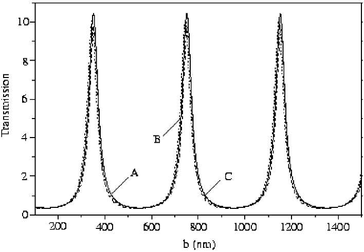
Figure 2: The transmission coefficient $T_{cw}$ for a continuous wave ($\omega$-Fourier component of a wave-packet) as a function of screen thickness $b$ computed for the wavelength $\lambda$=800 nm and the slit width $2a$ = 25 nm. Curve A, B and C correspond to the numerical near-field formula (35), the analytical near-field formula (36) and the analytical far-field formula (39), respectively. For computational reasons, in the case of curve C the limits of the integral were chosen to -1000$\lambda$ and 1000$\lambda$ instead of $-\infty$ and $\infty$; the computation was performed at $z=-10\lambda$.

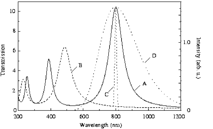
Figure 3: The dispersion $T_{cw}=T_{cw}(\lambda)$ for a continuous wave ($\omega$-Fourier component of a wave-packet) computed for the slit width $2a$ = 25 nm and different values of the screen thickness $b$: A - 350 nm and B - 200 nm. The Fourier spectra (curves C and D) are presented for the comparison. Curves C and D show the Fourier spectra of incident wave-packets with central wavelength $\lambda_{0}=$ 800 nm and duration ${\tau}=100$ fs and $\tau=5$ fs, respectively, which were used in the computations presented in Fig. 4 and 5.

where $S_{z}^{i}$ is the energy flux of the incident wave of unit amplitude; $S_{z}$ is the transmitted flux. Equation 35, which includes the evanescent modes that decay in the far zone, defines the transmission coefficient in the near-field zone. In order to establish guidelines for the results of our numerical analysis, we computed the transmission coefficient $T_{cw}({\lambda},a,b)$ for a continuous wave (Fourier $\omega$-component) as a function of screen thickness $b$ and/or wavelength $\lambda$ for different values of slit width $2a$. Throughout the computations, the magnitude of the incident magnetic field is assumed to be equal to 1. We consider a perfectly conducting nonmagnetic screen placed in vacuum ($\epsilon_{1}=\epsilon_{2}=\epsilon_{3}=1$) As an example, the dependence $T_{cw}=T_{cw}(b)$ computed for the wavelength $\lambda$ = 800 nm and the slit width $2a$ = 25 nm is shown in Fig. 2. The dispersion $T_{cw}=T_{cw}(\lambda)$ for $2a$ = 25 nm and different values of the screen thickness $b$ is presented in Fig. 3. In Fig. 2, we note the transmission resonances of $\lambda$/2 periodicity with the peak heights $T_{cw}{\approx}{\lambda}/{2\pi}a$ at the resonances. Notice that the resonance positions and the peak heights are in agreement with the results Harr ; Betz1 . The resonance peaks appear with spacing of 400 nm, but at values somewhat smaller than 400, 800, 1200 nm, etc. In order to better understand the shift of the resonant wavelengths from the naively expected values we have derived a simple analytical formula (36) for the transmission coefficient $T_{cw}~{}=~{}T_{cw}(a,b,\lambda)$ of a narrow slit (the fundamental mode only is retained):

$$T_{cw}(a,b,\lambda)=\frac{a}{2\frac{\pi}{\lambda}}\left[\left(\mathrm{Re}\left(D\left(b,\lambda\right)\right)\right)^{2}+\left(\mathrm{Im}\left(D\left(b,\lambda\right)\right)\right)^{2}\right]$$ (36)

, where

$$D(b,\lambda)=\frac{4}{2i\frac{\pi}{\lambda}}\left[\left[\exp\left(2ib\frac{\pi}{\lambda}\right)\left(A(\lambda)-\frac{i}{2\pi/\lambda}\right)\right]^{2}-\left(A(\lambda)+\frac{i}{2\pi/\lambda}\right)^{2}\right]^{-1}$$ (37)

and

$$A(\lambda)=ia\left[H_{0}^{(1)}\left(\lambda\right)+\frac{\pi}{2}\left(\mathbf{H}_{0}\left(\lambda\right)\cdot H_{1}^{(1)}\left(\lambda\right)+\mathbf{H}_{1}\left(\lambda\right)\cdot H_{0}^{(1)}]\left(\lambda\right)\right)\right]$$ (38)

In Eq. 38, $H_{0}^{(1)}(\lambda)$ and $H_{1}^{(1)}(\lambda)$ are the Hankel-functions, while $\mathbf{H}_{0}(\lambda)$ and $\mathbf{H}_{1}(\lambda)$ are the Struve-functions. It is interesting to compare the ”near-field” ($z<<\lambda$) transmittance with the conventional ”far-zone” ($z>>\lambda$) transmittance measured in experiments. The transmittance in the far-field zone can be described by the following formula:

$$T_{cw}=-\frac{\sqrt{\epsilon_{1}}}{4a}\int_{-\infty}^{\infty}{\lim_{z\rightarrow{0^{-}}}}[(E_{x}H_{y}^{*}+E_{x}^{*}H_{y})]dx,$$ (39)

Figure 2 compares the transmission coefficients $T_{cw}=T_{cw}(b)$ calculated by using the formula (36) with the values given by the numerical solution of the equations (24-II, 35) and the values obtained from the evaluation of (39). We notice that the results are practically undistinguishable. Analysis of the denominator of the formula (36) indicates that for $2a/\lambda$ small enough, the transmission $T_{cw}~{}=~{}T_{cw}(b)$ will exhibit the maximums around wavelengths $\sim$ $\lambda$/2. The shifts of the resonance wavelengths from the value $\lambda$/2 are caused by the wavelength dependent terms in the denominator of Eq. 36.

The dispersion $T_{cw}=T_{cw}(\lambda)$ presented in Fig. 3 indicates the wave-slit interaction behaviour, which is similar to those of a Fabry-Perot resonator. The transmission resonance peaks, however, have a systematic shift towards longer wavelengths. Analysis of the denominator of the formula (36) indicates that for $2a/\lambda$ small enough, the transmission $T_{cw}~{}=~{}T_{cw}(\lambda)$ will exhibit the Fabry-Perot like maximums around wavelengths where $\sin(kb)$ is zero. Such a behaviour has already been described in refs. Hibb ; Yang ; Taka . The shifts of the resonance wavelengths from the Fabry-Perot resonances are caused by the wavelength dependent terms in the denominator of Eq. 36. It should be noted that the values of the shifts calculated using Eq. 36 are in good agreement with the shifts calculated using the analytical formula (8) of the study  Taka . Our computations showed that the peak heights at the main (strongest) resonant wavelength $\lambda_{0}^{R}$ (in the case of Fig. 3, $\lambda_{0}^{R}$= 500 or 800 nm) are given by $T_{cw}(\lambda_{0}^{R},a){\approx}{\lambda_{0}^{R}}/{2\pi}a$. Notice that the Fabry-Perot like behaviour of the transmission coefficient is in agreement with analytical and experimental results published earlier Taka ; Yang . The enhancement coefficient ($T_{cw}\sim 30$) calculated using Eqs. 35 and 36, however, is different from the attenuation ($T_{cw}~{}<~{}1$) predicted by the study  Taka . The one order difference between the experimental value and the enhancement calculated in the present article is attributed to the small transverse dimension $D$ ($D\sim\lambda/2$) of the metal plates that form the slit. In our calculations we studied a slit in infinite transverse dimension ($D~{}=~{}\infty$).

Analysis of Fig. 3 indicates that a minimum thickness of the screen is required to get the waveguide resonance inside the slit at a given wavelength. The result is in agreement with the study  Taka , which demonstrated that there is no transmission peaks at the condition $b~{}<~{}\lambda/2$. Notice that the transmission enhancement mediated by surface plasmons does exist at considerably smaller thicknesses of the metal in comparison with the thickness required for the waveguide resonance. The surface plasmons/polaritons are excited in the skin, the depth of which is about the extinction length of the energy decay of electromagnetic wave in the metal. For instance, the extinction length in an aluminum screen is $\sim$ 4 nm for $\lambda$ = 800 nm. Therefore, for not too narrow slits (2$a$ = 25 nm) in thick screens ($b$ = 200 and 350 nm) considered in the paper, the finite skin depth does not fundamentally modify the process of the extraordinary optical transmission. At the wavelength 800 nm, the 10-times enhancement ($T_{cw}(a,\lambda)$ $\approx$ $\lambda/2\pi{a}$ $\approx$ 10) is limited by the slit width ($2a$ = 25 nm). In the far-infrared region ($\lambda$ $\approx$ 100 $\mu$m) several orders of magnitude enhancement can be achieved at the same experimental conditions. It should be noted that the optimal choice of parameters has been discussed in the literature and the obtained enhancement by the factors 10 and 1000 are typical for continuous waves in the optical and far-infrared spectral ranges. In the case of narrower and thinner slits, however, the influence of the finite conductivity effects on the transmission and localization of a pulse should be taken into account  Betz1 ; Taka .

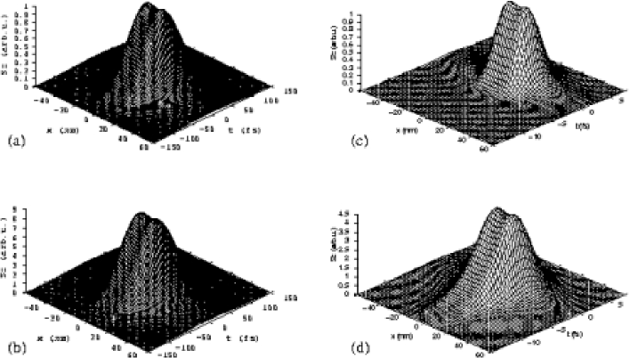
Figure 4: The energy flux of a transmitted pulse at the distance $|z|$ = $a/2$. (a), (c) The non-resonant transmission by the slit ($2a$ = 25 nm, $b$ = 200 nm; $\tau~{}=100$ fs and 5 fs, respectively). (b), (d) The resonant transmission by the slit ($2a$ = 25 nm, $b$ = 350 nm; $\tau=100$ fs and 5 fs, respectively). The central wavelength of the incident wave-packet is $\lambda_{0}=$ 800 nm.

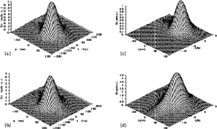
Figure 5: The energy flux of a transmitted pulse at the distance $|z|$ = $a$. (a), (c) The non-resonant transmission by the slit ($2a$ = 25 nm, $b$ = 200 nm; $\tau~{}=100$ fs and 5 fs, respectively). (b) The resonant transmission by the slit ($2a$ = 25 nm, $b$ = 350 nm; $\tau~{}=100$ fs and 5 fs, respectively). The central wavelength of the incident wave-packet is $\lambda_{0}=$ 800 nm.

The existence of transmission resonances for Fourier $\omega$-components of a wave-packet leads to the question: What effect the resonant enhancement has on the spatial and temporal localization of a light pulse? Presumably, the high transmission at resonance occurs when the system efficiently channels Fourier-components of the wave-packet from a wide area through the slit. At resonance, one might assume that if the energy flow is symmetric about the screen, the pulse width and duration should increase very rapidly past the screen. Thus the large pulse strength associated with resonance could only be obtained at the expense of the spatial and temporal broadening of the wave-packet. To test this hypothesis, the spatial distributions of the energy flux of a transmitted wave-packet were computed for different slit thicknesses corresponding to the resonance and anti-resonance position. The characteristic difference between the resonant and non-resonant transmissions could be understood better through a single figure of the field distributions in all regions I, II and III. However, it seems to be impossible to do this, because the visualization of a pulse by a single figure requires a 4-dimensional (U, x, z, t) coordinate system or a great number of 3-dimensional figures at different locations and suitable fixed times in all the regions. Therefore we present the eight 3-dimensional distributions (4(a)-(d) and 5(a)-(d)) only in the zone of main interest (region III). As an example, Figs. 4 (a) and 5 (a) show the energy flux of the anti-resonantly transmitted pulses. Figures 4 (b) and 5 (b) correspond to the case of the waveguide-mode resonance in the slit. Figures 4 and 5 show the transmitted pulses at the distances $|z|$ = $a/2$ and $a$, respectively. The rigorous analysis Betz1 showed that the number of modes required for the accurate computation of the transmittance, near-field distribution, and other optical characteristics of the system is given by $N~{}>~{}2a/z$, where N is the number of the waveguide modes and z is the distance from the screen. Therefore at the distances $|z|$ = $a/2$ and $a$ the calculations required at least 4 and 2 modes, respectively.

The shape and intensity of an output pulse depends on the slit parameters and the spectral width of the pulse. For narrow slits, the spectral width of a 100-fs input pulse is smaller compared to the spectral width of the resonant transmission (see, Fig. 3). The comparison of the flux distribution presented in Fig. 4 (a) with that of Fig. 4 (b) shows that, for the parameter values adopted, a transmitted wavepacket is enhanced by one order of magnitude and simultaneously localized in the 25-nm and 100-fs domains of the near-field diffraction zone. The shapes of the intensity distributions of the output pulses are very much the same off and on resonance. The figures differ only in the order of magnitude of $S_{z}$. Thus at the distance $|z|$ = $a/2$, the slit resonantly enhances the intensity of the pulse without its spatial and temporal broadening. The result can be easily understood by considering the dispersion properties of the slit. For the screen thickness $b$ = 200 nm, the amplitudes of the Fourier-components of the wave-packet, whose central wavelength $\lambda_{0}$ is detuned from the main (at 500 nm) resonance, are practically unchanged in the wavelength region near 800 nm (see, curve B in Fig. 3). This provides the dispersion- and distortion-free non-resonant transmission of the wave-packet (Figs. 4(a) and 5(a)). In the case of the thicker screen (b = 350 nm), the slit transmission experiences strong mode-coupling regime at the wavelengths near to 800 nm (see curve A of Fig. 3) that leads to a profound and uniform enhancement of amplitudes of all of the Fourier $\omega$-components of the wave-packet (see curve C in Fig. 3). Thus, the slit resonantly enhances by one order of magnitude the intensity of the pulse without its spatial and temporal broadenings (Figs. 4(b) and 5(b)). Also, notice that at the distance $|z|$ = $a$ (Figs. 5(a) and 5(b)), both the resonantly and anti-resonantly transmitted pulses experience natural spatial broadening in the transverse direction, while their durations are practically unchanged. The spectral width of a 5-fs input pulse, however, is bigger than the spectral width of the resonant transmission (Fig. 3). In this case the durations of the resonantly transmitted 5-fs pulses are longer in comparison with the pulses transmitted off the resonance (Figs. 4(c), (d) and respectively 5(c), (d)). We also notice that the enhancement of the intensity of 5-fs pulses is approximately two times lower in comparison with the 100-fs pulses. The temporal broadening of the pulse and the decrease of the enhancement indicates a natural limitation for the simultaneous temporal and spatial localization of a pulse together with its enhancement.

By comparing the data for anti-resonant and resonant transmissions presented in Figs. 4 and 5 one can see that at the appropriate values of the distance $|z|$ and the wave-packet spectral width $\Delta{\omega}$ the resonance effect does not influence the spatial and temporal localization of the wave-packet. To verify this somewhat unexpected result, the FWHMs of the transmitted pulse in the transverse and longitudinal directions were calculated for different values of the slit width $2a$, central wavelength $\lambda_{0}$ and pulse duration ${\tau}{\approx}1/\Delta{\omega}_{p}$ as a function of screen thickness $b$ at two particular near-field distances $|z|$ = $a/2$ and $a$ from the screen. It was seen that, at the dispersion-free resonant transmission condition $\Delta{\omega}_{p}~{}<~{}\Delta{\omega}_{r}$, the transmitted pulse indeed does not experience temporal broadening. Thus the temporal localization associated with the duration $\tau$ of the incident pulse remains practically unchanged under the transmission. The value of $\tau$ is determined by the dispersion-free condition ${\tau}{\approx}1/\Delta{\omega}_{p}>1/\Delta{\omega}_{r}$, where $\Delta{\omega}_{r}=\Delta{\omega}_{r}(a)$ practically does not depend on the screen thickness $b$. We found that the energy flux of the transmitted wave-packet can be enhanced by a factor $T_{cw}(\lambda_{0}^{R},a){\approx}{\lambda_{0}^{R}}/{2\pi}a$ by the appropriate adjusting of the screen thickness $b=b(\lambda_{0}^{R})$, for an example see Figs. 3-5. Thus the wave-packet can be enhanced by a factor ${\lambda_{0}^{R}}/{2\pi}a$ and simultaneously localized in the time domain at the ${\tau}={\tau}(a)$ scale. It was also seen that the FWHM of the transmitted pulse in the transverse direction depends on the wave-packet central wavelength $\lambda_{0}$ and the distance $z$ from the slit. Nevertheless, the FWHM of the transmitted pulse can be always reduced to the value $2a$ by the appropriate decreasing of the distance $|z|$ = $|z(a)|$ from the screen ($|z|$ = $a/2$, in the case of Fig. 4). Thus high transmission can be achieved without concurrent loss in the degree of temporal and spatial localizations of the pulse. In retrospect, this result is reasonable, since the symmetry of the problem for a time-harmonic continuous wave (Fourier $\omega$-component of a wave-packet) is disrupted by the presence of the initial and reflected fields in addition to the diffracted field on one side (Eq. 6). As the thickness changes, the fields $U^{d}$ and $U_{3}$ change only in magnitude, but the field $U_{1}$ changes in distribution as well since it involves the sum of $U^{d}$ with unchanging fields $U^{i}$ and $U^{r}$. At resonance, the distribution of $U_{1}$ leads to channeling of the radiation, but the distribution of $U_{3}$ remains unaffected. By the appropriate adjusting of the slit-pulse parameters a light pulse can be enhanced by orders of magnitude and simultaneously localized in the near-field diffraction zone at the nm- and fs-scales.

The limitations of the above analysis must be considered before the results are used for a particular experimental device. The resonant enhancement with simultaneous nm-scale spatial and fs-scale temporal localizations of a light by a subwavelength metal nano-slit is a consequence of the assumption of the screen perfect conductivity. The slit can be made of perfectly conductive (at low temperatures) materials. In the context of current technology, however, the use of conventional materials like metal films at a room temperature is more practical. Notice that a metal can be considered as a perfect conductor in the microwave range. As a general criterion, the perfect conductivity assumption should remain valid as far as the slit width and the screen thickness exceed the extinction length for the Fourier $\omega$-components of a wavepacket within the metal. The light intensity decays in the metal screen at the rate of $I_{s}~{}=~{}I_{0}~{}{\exp}(-b/{\delta})$, where ${\delta}$ = ${\delta}(\lambda)$ is the extinction length in the screen. The aluminum has the largest opacity ($\delta<$ 11 nm) in the spectral region $\lambda~{}>$ 100 nm [20]. The extinction length increases from 11 to 220 nm with decreasing the wavelength from 100 to 50 nm. Hence, the perfect conductivity is a very good approximation in a situation involving a relatively thick ($b~{}>$ 25 nm) aluminum screen and a wave-packet of the duration ${\tau}{\approx}1/\Delta{\omega}_{p}$ having the Fourier components in the spectral region $\lambda~{}>$ 100 nm. However, in the case of thinner screens, shorter pulses and smaller central wavelengths of wave-packets, the metal films are not completely opaque. This would reduce a value of spatial localization of a pulse due to passage of the light through the screen in the region away from the slit. Moreover, the phase shifts of the Fourier components along the propagation path caused by the skin effect can modify the enhancement coefficient and temporal localization properties of the slit.

The above analysis is directly applicable to the two-dimensional near-field scanning optical microscopy and spectroscopy. Although the computations were performed in the case of normal incidence, the preliminary analysis shows that in the case of oblique incidence the enhancement effect can be kept without further spatial and temporal broadening of the pulse. In a conventional 2D NSOM, a subwavelength ($2a~{}<~{}\lambda$) slit illuminated by a continuous wave is used as a near-field ($|z|<a$) light source providing the nm-scale resolution in space Ash ; Lewi ; Betz1 ; Pohl . The non-resonant transmission of fs pulses could provide ultrahigh resolution of 2D NSOM simultaneously in space and time Kuk1 ; Kuk2 . The above-described resonantly enhanced transmission together with nm- and fs-scale localizations in the space and time of a pulse could greatly increase the potentials of the 2D near-field scanning optical microscopy and spectroscopy, especially in high-resolution applications. However, as a model for a NSOM-tip a hole (quadratic, rectangular or circular) would be more appropriate than a slit-type waveguide. The consequences of the limitation of region II also in y-direction will result in faster attenuation of the amplitude of the waveguide modes compared to the slit-type waveguide modes  Betz1 . This should affect the enhancement and spatial and temporal broadening of the pulse. Moreover, the walls of the 2D slit have to be parallel over all the thickness to provide the resonance enhancement effect. Pulled NSOM 3D-tips, however, usually have conical ends. In the case of the tapered NSOM 3D waveguides one should also take into account the decrease of enhancement effect with increasing the waveguide taper. It should be also noted that the high transmission ($T_{cw}(\lambda_{0}^{R},a){\approx}{\lambda_{0}^{R}}/{2\pi}a$) of a pulse can be achieved without concurrent loss in the temporal and spatial localizations of the pulse only at short ($|z|=|z(a)|$) distances from the slit. The presence of a microscopic sample (a molecule, for example) placed at the short distance in strong interaction with NSOM slit modifies the boundary conditions. In the case of strong slit-sample-pulse interaction, which takes place at the distance $|z|<<0.1a$, the response function accounting for the modification of the quantum mechanical behaviour of the sample should be taken into consideration. The potential applications of the effect of the resonantly enhanced transmission together with nm- and fs-scale localizations of a pulse are not limited to near-field microscopy and spectroscopy. Broadly speaking, the effect concerns all physical phenomena and photonic applications involving a transmission of light by a single subwavelength nano-slit, a grating with subwavevelength slits and a subwavelength slit surrounded by parallel grooves (see the studies Neer ; Harr ; Betz1 ; Ash ; Lewi ; Betz2 ; Pohl ; Ebbe ; Leze ; Port ; Hibb ; Gar1 ; Gar2 ; Dog ; Li ; Stoc ; Kuk1 ; Kuk2 ; Stav ; Bori ; Taka ; Yang ; Cschr ; Trea ; Salo ; Cao ; Smol ; Barb ; Alte ; Dykh ; Stee ; Nawe ; Sun ; Shi ; Scho ; Naha ; Gome and references therein). For instance, the effect could be used for sensors, communications, optical switching devices and microscopes.

IV Conclusion

In the present article we have considered the question whether a light pulse can be enhanced and simultaneously localized in space and time by a subwavelength metal nano-slit. To address this question, the spatial distributions of the energy flux of an ultrashort (fs) pulse diffracted by a subwavelength (nanosized) slit in a thick metal screen of perfect conductivity have been analyzed by using the conventional approach based on the Neerhoff and Mur solution of Maxwell’s equations. The analysis of the spatial distributions for various regimes of the near-field diffraction demonstrated that the energy flux of a wavepacket can be enhanced by orders of magnitude and simultaneously localized in the near-field diffraction zone at the nm- and fs-scales. The extraordinary transmission, together with nm- and fs-scale localizations of the light pulse, make the nano-slit structures attractive for many photonic purposes, such as sensors, communication, optical switching devices and NSOM. We also believe that the addressing of the above-mentioned basic question gains insight into the physics of near-field resonant diffraction.

- (1) F. L. Neerhoff, G. Mur G, Appl. Sci. Res. 28, 73 (1973).
- (2) R.F. Harrington, D.T. AucklandJ, IEEE Trans. Antennas Propag AP28, 616 (1980).
- (3) E. Betzig, A. Harootunian, A. Lewis, M. Isaacson, Appl. Opt. 25, 1890 (1986).
- (4) E.A. Ash, G. Nicholls, Nature (London) 237, 510 (1972).
- (5) A. Lewis, K. Lieberman, Nature (London) 354, 214 (1991).
- (6) E. Betzig, J.K. Trautman, T.D. Harris, J.S. Weiner, R.L. Kostelak, Science 251, 1468 (1991).
- (7) D.W. Pohl, D. Courjon, Eds., Near Field Optics, NATO ASI Series E Vol. 242 (The Netherlands, Dordrecht: Kluwer, 1993).
- (8) T.W. Ebbesen, H.J. Lezec, H.F. Ghaemi, T. Thio, P.A. Wolff, Nature (London) 391, 667 (1998).
- (9) H.J. Lezec, A. Degiron, E. Devaux, R.A. Linke, Martin-Moreno, F.J. Garcia-Vidal, T.W. Ebbesen, Science 297, 820 (2002).
- (10) J. A. Porto, F.J. Garcia-Vidal, J.B. Pendry, Phys. Rev. Lett. 83, 2845 (1999).
- (11) A.P. Hibbings, J.R. Sambles, C.R. Lawrence, Appl. Phys. Lett. 81, 4661 (2002).
- (12) F.J. Garcia-Vidal, H.J. Lezec, T.W. Ebbesen, L. Martin-Moreno, Phys. Rev. Lett. 90, 231901 (2003).
- (13) F.J. Garcia-Vidal, L. Martin-Moreno, H.J. Lezec, T.W. Ebbesen, Appl. Phys. Lett. 83, 4500 (2003).
- (14) A. Dogariu, M. Hsu, L.J. Wang, Opt. Comm. 220, 223 (2003).
- (15) K.R. Li, M.I. Stockman, D.J. Bergman, Phys. Rev. Lett. 91, 227402 (2003).
- (16) M.I. Stockman, S.V. Faleev, D.J. Bergman, Phys. Rev. Lett. 88, 067402 (2002).
- (17) S.V. Kukhlevsky, M. Mechler, L. Csapo, K. Janssens, Phys. Lett. A 319, 439 (2003).
- (18) S.V. Kukhlevsky, M. Mechler, Opt. Comm. 231, 35 (2004).
- (19) P. N. Stavrinou, Phys. Rev. E 68, 06604 (2003).
- (20) A.G. Borisov, S.V. Shabanov, arXiv:physics/0312103 (2003).
- (21) Y. Takakura, Phys. Rev. Lett. 86, 5601 (2001).
- (22) F.Z. Yang, J.R. Sambles, Phys. Rev. Lett. 89, 063901 (2002).
- (23) U. Schroter, D. Heitmann, Phys. Rev. B 58, 15419 (1998).
- (24) M.M.J. Treacy, Phys. Rev. Lett. 75, 606 (1999).
- (25) L. Salomon, F.D. Grillot, A.V. Zayats, F. de Fornel, Phys. Rev. Lett. 86, 1110 (2001).
- (26) Q. Cao, P. Lalanne, Phys. Rev. Lett. 88, 057403 (2002).
- (27) I.I. Smolyaninov, A.V. Zayats, A. Stanishevsky, C.C. Davis, Phys. Rev. B 66, 205414 (2002).
- (28) A. Barbara, P. Quemerais, E. Bustarret, T. Lopez-Rios, Phys. Rev. B 66, 161403 (2002).
- (29) E. Altewischer, M.P. van Exter, J.P. Woerdman, Nature (London) 418, 304 (2002).
- (30) A.M. Dykhne, A.K. Sarychev, V.M. Shalaev, Phys. Rev. B 67, 195402 (2003).
- (31) J.M. Steele, C.E. Moran, A. Lee, C.M. Aguirre, N.J. Halas, Phys. Rev. B 68, 205103 (2003).
- (32) A. Naweed, F. Baumann, W.A. Bailey, A.S. Karakashian, W.D. Goodhue, J. Opt. Soc. Am. B 20, 2534 (2003).
- (33) Z.J. Sun, Y.S. Jung, H.K. Kim, Appl. Phys. Lett. 83, 3021 (2003).
- (34) X.L. Shi, L. Hesselink, R.L. Thornton, Opt. Lett. 28, 1320 (2003).
- (35) H.F. Schouten, T.D. Visser, D. Lenstra, H. Blok, Phys. Rev. E 67, 036608 (2003).
- (36) A. Nahata, R.A. Linke, T. Ishi, K. Ohashi, Opt. Lett. 28, 423 (2003).
- (37) G. Gomez-Santos, Phys. Rev. Lett. 90, 077401 (2003).