Exactly Integrable Dynamics of Interface between Ideal Fluid and Light Viscous Fluid

Abstract

It is shown that dynamics of the interface between ideal fluid and light viscous fluid is exactly integrable in the approximation of small surface slopes for two-dimensional flow. Stokes flow of viscous fluid provides a relation between normal velocity and pressure at interface. Surface elevation and velocity potential of ideal fluid are determined from two complex Burgers equations corresponding to analytical continuation of velocity potential at the interface into upper and lower complex half planes, respectively. The interface loses its smoothness if complex singularities (poles) reach the interface.

Dynamics of an interface between two incompressible fluids is an important fundamental problem which has numerous applications ranging from interaction between see and atmosphere to flow through porous media and superfluids. If one neglects gravity and surface tension, that problem can be effectively solved in some particular cases in two dimensions with the use of complex variables. Integrable cases include Stokes flow of viscous fluid with free surface Richardson1968 , dynamics of free surface of ideal fluid with infinite depth KuznetsovSpektorZakharov1994 and finite depth DyachenkoZakharovKuznetsov1996 , dynamics of an interface between two ideal fluids KuznetsovSpektorZakharov1993 , ideal fluid pushed through viscous fluid in a narrow gap between two parallel plates (Hele-Shaw flow) Richardson1972 ; Kadanoff1986 ; Mineev1998 .

Here a new integrable case is found which corresponds to two-dimensional motion of the interface between heavy ideal fluid and light viscous fluid in absence of gravity and capillary forces. The interface position is given by $z=\eta(x,t)$, where the first, heavier fluid (indicated by index 1) with the density $\rho_{1}$ occupies the region $-\infty<z<\eta(x,t)$ and the second, lighter fluid (index 2) with the density $\rho_{2}$ occupies the region $\eta(x,t)<z<\infty$.

Suppose that the kinematic viscosity of the fluid 2, $\nu_{2}$, is very large so that fluid’s 2 flow has small Reynolds numbers and, neglecting inertial effect in the Navier-Stokes Eq., one arrives to the Stokes flow Eq. landaufluid :

$$\nu_{2}\nabla^{2}{\bf v}_{2}-\frac{1}{\rho_{2}}\nabla p_{2}=0,\quad\nabla\cdot{\bf v}_{2}=0,$$ (1)

where ${\bf v}_{2}\equiv(v_{2,\,x},v_{2,\,z})$ is the velocity of the fluid 2, $\nabla=(\partial_{x},\partial_{z})$, and $p_{2}$ is the fluid’s 2 pressure (similar physical quantities for the fluid 1 have index 1 below). Additional assumption necessary for applicability of Eq. $(\ref{stokes1})$ is a small density ratio,

$$\rho_{2}/\rho_{1}\ll 1,\quad\rho_{1}\equiv 1,$$ (2)

which ensure that the fluid 2 responds very fast to perturbations of the interface as inertia of the fluid 2 is very small compare with fluid’s 1 inertia while time dependent perturbations of the fluid 2 decay very fast due to large viscosity $\nu_{2}$. According to Eq. $(\ref{stokes1})$, the response of the fluid 2 to motion of the interface is static. For any given normal velocity of the interface, $v_{n}$, Eq. $(\ref{stokes1})$ allows to determine the pressure $p_{2}|_{z=\eta}$ at the interface. In other words, the fluid 2 adiabatically follows the slow motion of the heavy fluid 1 and Reynolds number of the fluid 2 remains small at all time.

The velocity of the potential motion of ideal the fluid 1, ${\bf v}_{1}=\nabla\phi$, can be found from solution of the Laplace Eq., $\nabla^{2}\phi=0,$ which is a consequence of the incompressibility condition, $\nabla\cdot{\bf v}_{1}=0$, for potential flow. Boundary conditions at infinity are decaying, $|{\bf v}_{1}|,\,p_{1}\to 0\quad\mbox{for}\quad z\to-\infty;\\ |{\bf v}_{2}|,\,p_{2}\to 0\quad\mbox{for}\quad z\to+\infty.$

Motion of the interface is determined from the kinematic boundary condition of continuity of normal component of fluid velocity across the interface:

$$v_{n}\equiv v_{1\,n}|_{z=\eta}=v_{2\,n}|_{z=\eta}=\partial_{t}\eta\big{[}1+(\partial_{x}\eta)^{2}\big{]}^{-1/2},$$ (3)

where $v_{1(2)\,n}={\bf n}\cdot{\bf v}_{1(2)}$ and ${\bf n}=(-\partial_{x}\eta,1)\big{[}1+(\partial_{x}\eta)^{2}\big{]}^{-1/2}$ is the interface normal vector.

A dynamic boundary condition is a continuity of stress tensor, $\sigma_{1(2),\,jm}=-p_{1(2)}\delta_{jm}+\sigma_{1(2),\,jm}^{\prime},$ $\sigma_{1(2),\,jm}^{\prime}\equiv\rho_{1(2)}\nu_{1(2)}(\frac{\partial v_{1(2),\,m}}{\partial x_{j}}+\frac{\partial v_{1(2),\,j}}{\partial x_{m}})$, $x_{1}\equiv x,\ x_{2}\equiv z$, across the interface: $n_{j}\sigma_{1,\,jm}|_{z=\eta}=n_{j}\sigma_{2,\,jm}|_{z=\eta}$ (repetition of indexes $j,m$ means summation from 1 to 2), which gives two scalar dynamic boundary conditions:

$$p_{1}|_{z=\eta}=p_{2}|_{z=\eta}+n_{m}n_{j}\sigma^{\prime}_{2,\,jm}|_{z=\eta},$$

$$l_{m}n_{j}\sigma_{2,\,jm}^{\prime}|_{z=\eta}=0,$$ (4)

where the absence of viscous stress in the ideal fluid 1, $\nu_{1}=0,$ is used, $n_{m},l_{m}$ are components of the interface normal vector, ${\bf n},$ and the interface tangential vector, ${\bf l}=(1,\partial_{x}\eta)\big{[}1+(\partial_{x}\eta)^{2}\big{]}^{-1/2}.$ The pressure $p_{1}$ of the fluid 1 at the interface can be determined from a nonstationary Bernoulli Eq., $\big{[}\partial_{t}\phi+\frac{1}{2}(\nabla\phi)^{2}+\frac{p_{1}}{\rho_{1}}\big{]}\Big{|}_{z=\eta}=0.$

To obtain a closed expression for interface dynamics in terms of fluid’s 1 variables only, one can first find an expression for the pressure at the interface through the normal velocity $v_{n}$ .

It follows from Eq. $(\ref{stokes1})$ that $\nabla^{2}p_{2}=0$ and the Fourier transform over $x$ allows to write the solution of the Laplace Eq. with the decaying boundary condition at $x\to\infty$ as $p_{2\,k}(z)=p_{2\,k}(0)\exp(-|k|z)\equiv\int dx\,p_{2}(x,z)\exp(-ikx)$.

To determine ${\bf v}_{2}|_{z=\eta}$ one can introduce a shift operator, $\hat{L}_{2}$, defined from series expansion: ${\bf v}_{2}(x,z)\big{|}_{z=\eta}\equiv\hat{L}_{2}{\bf v}_{2}(x,0)=\Big{[}(1+\eta\partial_{z}+\frac{1}{2}\eta^{2}\partial^{2}_{z}+\ldots){\bf v}_{2}(x,z)\Big{]}\Big{|}_{z=0}$ and use Eq. $(\ref{stokes1})$ to find $v_{2,\,x\,k}(z)=\Big{[}c_{k}-ikz\frac{p_{2\,k}(0)}{2\rho_{2}\nu_{2}|k|}\Big{]}\exp(-|k|z),$ $v_{2,\,z\,k}(z)=\Big{[}i\,\mbox{sign}(k)c_{k}+(|k|z+1)\frac{p_{2\,k}(0)}{2\rho_{2}\nu_{2}|k|}\Big{]}\exp(-|k|z),$ where $v_{2,\,x\,k}(z),\ v_{2,\,z\,k}(z)$ are the Fourier transform over $x$ of the components of the velocity ${\bf v}_{2}$ and functions $c_{k}$, $p_{2\,k}(0)$ should be determined from the dynamic boundary conditions $(\ref{dyn1})$.

Operator $\hat{L}_{2}$ can be expressed, using Eq. $(\ref{stokes1})$, in terms of the operator $\hat{k}:$ $\hat{L}_{2}=1-\eta\hat{k}+\frac{1}{2}\eta^{2}\hat{k}^{2}+\ldots,$ where the integral operator $\hat{k}$ is an inverse Fourier transform of $|k|$ and is given by

$$\hat{k}=-\frac{\partial}{\partial x}\hat{H}.$$ (5)

Here $\hat{H}f(x)=\frac{1}{\pi}P.V.\int^{+\infty}_{-\infty}\frac{f(x^{\prime})}{x^{\prime}-x}dx^{\prime}$ is the Hilbert transform and $P.V.$ means Cauchy principal value of integral. $\hat{H}$ can be also interpreted as a Fourier transform of $i\,\mbox{sign}(k)$.

In a similar way one can show that $[\partial_{x}{\bf v}_{2}(x,z)]\big{|}_{z=\eta}=\hat{L}_{2}\partial_{x}{\bf v}_{2}(x,0),$ $[\partial_{z}v_{2,\,x}(x,z)]\big{|}_{z=\eta}=-\hat{L}\hat{k}v_{2,\,x}(x,0)-\frac{1}{2\nu_{2}\rho_{2}}\hat{L}_{2}\hat{k}^{-1}\partial_{x}p_{2}(x,0),$ $p_{2}(x,\eta)=\hat{L}_{2}p_{2}(x,0)$ and using kinematic $(\ref{vn1vn2})$ and dynamic $(\ref{dyn1})$ boundary conditions one can find $p_{1}(x,\eta)$ as a linear functional of $v_{n}$. That linear functional can be expressed in a form of powers series with respect to small parameter $|\partial_{x}\eta|$, which has a meaning of typical slope of the interface inclination relative to the interface undisturbed (plane) position.

At leading order approximation over small parameter $|\partial_{x}\eta|$ one gets: $p_{1}(x,\eta)=p_{2}(x,0),$ $v_{n}=v_{2,\,z}(x,\eta)$, and, respectively, response of pressure to normal velocity is given by

$$p_{1}|_{z=\eta}=2\rho_{2}\nu_{2}\hat{k}v_{n}.$$ (6)

In other words, Eq. $(\ref{vnp})$ determines a static response of the fluid 2 to the motion of the interface.

Eq. $(\ref{vnp})$ together with the kinematic boundary condition $(\ref{vn1vn2})$ and the Laplace Eq. for the velocity ponetial $\phi$ completely defines the potential motion of the fluid 1.

Following Zakharov Zakharov1968 , one can introduce the surface variable $\psi(x)\equiv\phi(x,\eta),$ which is the value of the velocity potential, $\phi(x,z)$, at the interface. Kinematic boundary condition $(\ref{vn1vn2})$ can be written at leading order over small parameter $|\partial_{x}\eta|$ as

$$\partial_{t}\eta=-\hat{H}v,$$ (7)

where a new function, $v=\partial_{x}\psi,$ is introduced which has a meaning of the tangent velocity of the fluid 1 at the interface.

Similar to the shift operator $\hat{L}_{2},$ one can define a shift operator, $\hat{L}_{1}=1+\eta\hat{k}+\frac{1}{2}\eta^{2}\hat{k}^{2}+\ldots,$ which corresponds to the harmonic function $\phi$ with vanishing boundary condition $\phi\to 0$ for $z\to-\infty$. A Fourier transform of $\phi$, $\phi_{k}(z)=\phi_{k}(0)\exp(|k|z)$, allows to find the components of fluid velocity at the interface: $(\partial_{x}\phi)\big{|}_{z=\eta}=\hat{L}_{1}\partial_{x}\phi(x,0)=\hat{L}_{1}\partial_{x}\hat{L}_{1}^{-1}\psi,\ (\partial_{z}\phi)\big{|}_{z=\eta}=\hat{L}_{1}\hat{k}\hat{L}_{1}^{-1}\psi$ through surface variables $\eta,\,\psi$. Time derivative $\phi_{t}$ in the nonstationary Bernoulli can be found from $\partial_{t}\psi=\partial_{t}\phi|_{z=\eta}+\partial_{t}\eta\partial_{z}\phi|_{z=\eta}$ and one gets at leading order approximation over $|\partial_{x}\eta|$:

$$\frac{\partial v}{\partial t}-\frac{1}{2}\partial_{x}\Big{[}(\hat{H}v)^{2}-v^{2}\Big{]}=2\nu_{2}\rho_{2}\partial_{x}^{2}v.$$ (8)

Note that Eq. $(\ref{vtot})$ does not include variable $\eta$ which is a peculiar property of lowest perturbation order over $|\partial_{x}\eta|$.

Because the surface tension and gravity is neglected here, the total energy of two fluid equals to total kinetic energy, $K$. $K$ decays, $\frac{dK}{dt}\simeq-\frac{\nu_{2}\rho_{2}}{\pi}\int dk|k|^{3}|\psi_{k}|^{2}<0,$ due to dissipation in the fluid 2. If the fluid 2 is absent, which corresponds to $\rho_{2}=0$, then $K$ is conserved, $\frac{dK}{dt}=0$, and the motion of the fluid 1 can be expressed in the standard Hamiltonian form Zakharov1968 ; KuznetsovSpektorZakharov1994 : $\frac{\partial\eta}{\partial t}=\frac{\delta K}{\delta\psi},$ $\frac{\partial\psi}{\partial t}=-\frac{\delta K}{\delta\eta}$.

Equations, similar to $(\ref{etavt}),(\ref{vtot})$ can be derived for three dimensional motion also with the main difference that the operator $\hat{k}$ in three dimensions is not given by $(\ref{kdef})$ but determined from the Fourier transform of $|k|$ over two horizontal coordinates. Subsequent analysis is however restricted to two dimensional fluid motion only.

The real function $v(x)$ can be uniquely represented as a sum of two complex functions $v^{(+)}$ and $v^{(-)}$, $v=[v^{(+)}+v^{(-)}]/2,$ which can be analytically continued from real axis $x$ into upper and lower complex half-planes, respectively. The Hilbert transform acts on these functions as $\hat{H}v^{(+)}=iv^{(+)},\quad\hat{H}v^{(-)}=-iv^{(-)}$ and Eq. $(\ref{vtot})$ splits into two decoupled complex Burgers Eqs. for $v^{(+)}$ and $v^{(-)}$:

$$\frac{\partial v^{(\pm)}}{\partial t}+v^{(\pm)}\partial_{x}v^{(\pm)}=\tilde{\nu}\partial_{x}^{2}v^{(\pm)},$$ (9)

where an effective viscosity, $\tilde{\nu}=2\nu_{2}\rho_{2}$ is introduced to make connection with the standard definition of real Burgers Eq. ColeHopf . Similar reduction of integro-differential Eq. (like Eq. $(\ref{vtot})$) to complex Burgers Eq. was done in Ref. Ablowitz1987 .

If the fluid 2 is absent, $\tilde{\nu}=0$, complex Burgers Eqs. $(\ref{vtotpm})$ are reduced to inviscid Burgers Eqs. (the Hopf Eqs.) which were derived for ideal fluid with free surface in Ref. KuznetsovSpektorZakharov1994 (note that definition of $v^{(\pm)}$ in this Letter differs from similar definition in Ref. KuznetsovSpektorZakharov1994 by a factor $1/2$). While viscosity $\nu_{2}$ is large enough to make sure that Reynolds number in the fluid 2, ${\bf R}_{2},$ is small, ${\bf R}_{2}\sim v_{n}/(\nu_{2}k)\ll 1$ ($k$ is a typical wave vector of surface perturbation) but effective viscosity $\tilde{\nu}$ can be small provided $\rho_{2}\ll{\bf R}_{2}\ll 1$ so that Reynolds number , ${\bf R},$ in complex Burgers Eq. $(\ref{vtotpm})$ is large, ${\bf R}\sim{\bf R}_{2}/\rho_{2}\gg 1.$

Complex Burgers Eq. is transformed into the complex heat Eq. $\frac{\partial u^{(\pm)}}{\partial t}=\tilde{\nu}\partial_{x}^{2}u^{(\pm)}$ via the Cole-Hopf transform ColeHopf : $v^{(\pm)}=-2\tilde{\nu}\frac{\partial_{x}u^{(\pm)}}{u^{(\pm)}}.$ Solution of the heat Eq. with initial data $u^{(\pm)}(x,t)\big{|}_{t=0}\equiv u_{0}^{(\pm)}(x)$, $u^{(\pm)}(x,t)=(4\pi\tilde{\nu}t)^{-1/2}\int^{\infty}_{-\infty}dx^{\prime}\exp\Big{[}-\frac{(x-x^{\prime})^{2}}{4\tilde{\nu}t}\Big{]}u_{0}^{(\pm)}(x^{\prime}),$ is an analytic function in complex $x$ plane for any $t>0$ because integral of right hand side (rhs) of this Eq. over any closed contour in complex $x$ plane is zero (Morera’s theorem). Then, according to the Cole-Hopf transform, solution of the complex Burgers Eq. can have pole singularities corresponding to zeros of $u^{(\pm)}(x,t)$. Number of zeros, $n(\gamma)$, of $u^{(\pm)}(x,t)$ (each zero is calculated according to its order) inside any simple closed contour $\gamma$ equals to $\frac{1}{2\pi i}\int_{\gamma}dx\partial_{x}u^{(\pm)}(x,t)/u^{(\pm)}(x,t)$. Integration of Eq. $(\ref{vtotpm})$ over $\gamma$ allows to conclude that $n(\gamma)$ is conserved as a function of time provided zeros do not cross $\gamma$. Thus number of zeros in entire complex plane can only change in time because zero can be created or annihilated at complex infinity, $x=\infty$, provided $u^{(\pm)}(x,t)$ has an essential singularity at complex infinity.

From physical point of view it is important that zeros of $u^{(\pm)}(x,t)$ can reach real axis $x=Re(x)$ which distinguishes the complex Burgers Eq. from the real Burgers Eq. Solution of the real Burgers Eq., which corresponds to Eq. $(\ref{vtotpm})$ with $v^{(\pm)}(x,t)\big{|}_{t=0}=Re\big{[}v^{(\pm)}(x,t)\big{|}_{t=0}\big{]}$, has global existence (remains smooth for any time), while solution of the complex Burgers generally exists until some zero of $u^{(\pm)}(x,t)$ hits real axis $x$ for the first time.

To make connection with inviscid case KuznetsovSpektorZakharov1994 one can look at initial condition for $v^{(+)}(x,0)$ with one simple pole in the lower half-plane:

$$v^{(+)}(x,0)=\frac{2A}{x+ia},\quad Re(a)>0.$$ (10)

Solution of the inviscid ($\tilde{\nu}=0)$ Burgers Eq. with initial condition $(\ref{simplepole})$ gives KuznetsovSpektorZakharov1994 : $v^{(+)}_{inviscid}(x,t)=\frac{4A}{x+ia+\sqrt{(x+ia)^{2}-8At}},$ which has two moving branch points: $x_{1,2}=-ia\pm 2\sqrt{2At}.$ One of these branch points reaches real axis in a finite time if either $A<0$ or $Re(A)\neq 0.$ As the branch point touches the real axis, the inviscid solution is not unique any more and the interface looses its smoothness KuznetsovSpektorZakharov1994 .

Consider now solution of the viscous Burgers Eq. $(\ref{vtotpm})$ with nonzero effective viscosity $\tilde{\nu}$ and with the simple pole conditions $(\ref{simplepole})$. Respectively, initial condition for the heat Eq., is given by $u_{0}^{(+)}=(x+ia)^{-A/\tilde{\nu}}$ and has branch point at $x=-ia$. Solution of the heat Eq. gives $u^{(+)}(x,t)=\exp\big{(}i\frac{\pi\tilde{\mu}}{2}\big{)}H_{\tilde{\mu}}\Big{(}-\frac{i}{2\sqrt{\tilde{\nu}t}}[x+ia]\Big{)},$ where $\tilde{\mu}\equiv-A/\tilde{\nu}$ and $H_{\mu}(z)$ is the Hermite function defined as $H_{\mu}(z)=\frac{2^{\mu+1}}{\sqrt{\pi}}e^{z^{2}}\int^{\infty}_{0}dye^{-y^{2}}y^{\mu}\cos\big{(}2zy-\frac{\pi\mu}{2}\big{)}.$ Zeros of $u^{(+)}(x,t)$ (and, equivalently, poles of $v^{(+)}(x,t)$) move in complex $x$ plane with time as (see Figure 1)

$$x_{j}(t)=i(2\sqrt{\tilde{\nu}t}z_{j}-a),$$ (11)

where $z_{1},z_{2},\ldots,$ are complex zeros of the Hermite function.

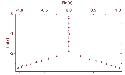
Figure 1: Motion of poles of the complex velocity, $v^{(+)}(x,t)$, in complex $x$ plane for $A=-1/8,\,\tilde{\mu}=7.6,\,\tilde{\nu}\simeq 0.0164,\,a=1,\ t=0.8.$ Arrows point out the position, direction and magnitude of moving poles. Uppermost arrow designates the pole which corresponds to zero of the Hermite function with the largest real part (that pole first reaches real axis for $t_{viscous}\simeq 1.91$ producing singularity of the interface surface). Dotted line connects two branch points (filled circles) of inviscid solution. Upper branch point reaches real axis for $t_{inviscid}=1$ which corresponds to singularity in the solution of the inviscid Burgers Eq. Empty circle designates the simple pole initial condition $(\ref{simplepole})$. Viscous solution becomes singular at later time compare to inviscid solution, $t_{viscous}>t_{inviscid}.$

Consider a particular case, $\tilde{\mu}=n,$ $n$ is a positive integer number. The Hermite function is reduced to the Hermite polynomial $H_{n}(z)$ which has $n$ zeros, $z_{1},z_{2},\ldots,z_{n}$ located at real axis $z=Re(z)$, $z_{n}$ corresponds to the largest zero. Location of real zeros of the Hermite function with real $\tilde{\mu}$ is close to location of zeros of the Hermite polinomial with the closest integer $n$ to the given $\tilde{\mu}$ while zeros with nonzero imaginary part (which corresponds to tails with nonzero real part in Figure 1) disappear for $\tilde{\mu}=n.$ Zeros of the Hermite polinomial are moving with time parallel to imaginary axis $x=Im(x)$ in complex $x$ plane according to $(\ref{xj})$ and the complex velocity $v^{(+)}$ is described by set of moving poles:

$$v^{(+)}=-2\tilde{\nu}\sum\limits_{j=1}^{n}\frac{1}{x-x_{j}(t)}.$$ (12)

$v^{(-)}$ is given by the same expression with $x_{j}$ replaced by their conjugated values $\bar{x}_{j}$.

Eqs. $(\ref{vtotpm})$ have also another wide class of solutions, “pole decomposition”, corresponding to Eq. $(\ref{vj})$ with $\frac{dx_{j}}{dt}=-2\tilde{\nu}\sum\limits_{l=1,\,j\neq l}^{n}\frac{1}{x_{j}-x_{l}}$, $n$ is arbitrary positive integer Choodnovsky1977 . Simple pole initial condition $(\ref{simplepole})$ with $\tilde{\mu}=n$ is particular case for which $x_{j}|_{t=0}=0$ for any $j$.

As $v(x,t)$ is known from solution of the heat Eq. and the Cole-Hopf transform one can find $\eta(x,t)$ from Eq. $(\ref{etavt})$. Interface dynamics is determined from the most rapid pole of $v^{(\pm)}$ which first reaches real axis, $x=Re(x)$. E.g., for initial condition $(\ref{simplepole})$, the pole singularity of $v^{(+)}$ first hits real axis, $x=Re(x)$, from below at time $t_{viscous}=\frac{Re(a)^{2}}{4\tilde{\nu}Re(z_{max})^{2}}$, where $z_{max}$ is a complex zero of the Hermite function with the largest real part for given $\tilde{\mu}$. Simultaneously, the pole singularity of $v^{(-)}$ first hits real axis from above at the same point.

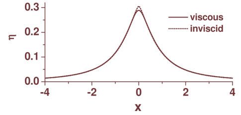
Figure 2: The interface position, $\eta(x,t)$, according to solution of Eqs. $(\ref{etavt}),(\ref{vtot})$ with finite viscosity, $\tilde{\nu}=1/64$ (solid line) and zero viscosity, $\tilde{\nu}=0,$ (dotted line) for $A=-1/8,\,\,a=1,\ t=1$. Viscous solution has 8 moving poles while inviscid solution is singular at $x=0$ ($\partial^{2}_{xx}\eta|_{x=0}\to-\infty$ as $t\to t_{inviscid}=1$). Both solutions are almost indistinguishable outside a small neighborhood around $x=0$. As $\tilde{\mu}$ increases, the viscous solution approaches invisicid.

Figure 2 shows $\eta(x)$ at the time, $t=t_{inviscid}$, when singularity (branch point) of inviscid solution first reaches the interface breaking analyticity of inviscid solution. It is seen that viscous solution significantly deviates from inviscid one only in the narrow domain around $x=0$.

Viscous solution remains analytic for $t>t_{inviscid}$ until $t<t_{viscous}$ ($t_{viscous}\simeq 1.91$ for parameters in Fig.1). However, for $t\to t_{viscous}$, surface elevation behaves as $\eta\simeq(-a/2z_{max}^{2})\log{\big{[}x^{2}+(2\sqrt{t\tilde{\nu}}z_{max}-a)^{2}\big{]}}$ near $x=0$ (it is set here $Im(a)=Im(A)=0$) meaning that small slope approximation used for derivation of Eqs. $(\ref{etavt}),(\ref{vtot})$ is violated for $t\to t_{viscous}$ and full hydrodynamic Eqs. should be solved near singularity. One can find a range of applicability of Eqs. $(\ref{etavt}),(\ref{vtot})$ by looking at correction to these Eqs. E.g. the analysis for parameters of Fig. 1 shows that the correction is important for $t\gtrsim 0.9t_{viscous}$ (for $t=0.9t_{viscous}$ correction to $\eta|_{x=0}$ is about $30\%.)$ Detail consideration of that question is outside the scope of this Letter. Note that the question whether an actual singularity of the interface surface occurs in full hydrodynamic Eqs. remains open.

To make connection with dynamics of ideal fluid with free surface (corresponds to the inviscid Burgers Eqs.) KuznetsovSpektorZakharov1994 one can consider a limit $\tilde{\nu}\to 0$ and, respectively, $\tilde{\mu}\to\infty$. It can be shown from the asymptotic analysis of the integral representation of the Hermite function that the largest zero, $z_{max},$ is given by $z_{max}=2^{1/2}\tilde{\mu}^{1/2}+O(\tilde{\mu}^{-1/6})$ The leading order term, $2^{1/2}\tilde{\mu}^{1/2}$, exactly corresponds to the position of the upper branch point of inviscid solution (see Fig. 1) while term $O(\tilde{\mu}^{-1/6})<0$ is responsible for the difference between $t_{inviscid}$ and $t_{viscous}$. Even for moderately small $\tilde{\nu}$ as in Fig. 1 that difference is numerically close to 1 because of small power $\tilde{\mu}^{-1/6}$.

It is easy to derive a wide class of initial conditions for which solution $(\ref{etavt}),(\ref{vtot})$ exists globally and the interface remains smooth at all times. E.g. one can take $u^{(+)}=a_{0}e^{ik_{0}x-\tilde{\nu}k_{0}^{2}t},$ $k_{0}=Re(k_{0})>0$ or any sum of imaginary exponent which ensure that there is no zeros at $Im(x)=0$. However, it we suppose that there is a random force pumping of energy into system (or random initial condition) then one can expect that some trajectories with nonzero measure would have poles which reach real axis in a finite time.

In conclusion, one can mention possible physical applications. Eqs. $(\ref{etavt}),(\ref{vtot})$ describe a free surface dynamics of Helium II with both normal ($\nu_{2}\neq 0$) and superfluid ($\nu_{1}=0$) components. Derivation of these Eqs. is slightly different from given in this Letter because both fluids occupy the same volume but resulting Eqs. are exactly the same as $(\ref{etavt}),(\ref{vtot})$. For classical fluids viscosity is nonzero but $\nu_{1}$ can be neglected and the fluid 1 can be considered as ideal fluid provided the ratio of dynamic viscosities of two fluids is large, $\nu_{2}\rho_{2}/(\nu_{1}\rho_{1})\gg 1$. E.g. that ratio is $\sim 900$ for glycerin and mercury while ratio of their densities is $\sim 0.09$ which makes them good candidates for experimental test of the analytical result of this Letter.

The author thanks M. Chertkov, I.R. Gabitov, E.A. Kuznetsov, H.A. Rose, and V.E. Zakharov for helpful discussions.

Support was provided by the Department of Energy, under contract W-7405-ENG-36.

References

(1) S. Richardson, J. Fluid Mech. 33, 475 (1968); S. Richardson, Eur. J. Appl. Maths 3, 193
(1992); S.D.Howison, and S. Richardson, Eur. J. Appl. Maths 36, 441 (1995).
(2) E.A. Kuznetsov, M.D. Spector and V.E. Zakharov, Phys. Rev. E
49, 1283 (1994).
(6) D. Bensimon, L.P. Kadanoff, S. Liang, B.I.
Shraiman, and C. Tang, Rev. Mod. Phys., 58, 977 (1986); P.
Konstantin, and L. Kadanoff, Physica D, 47, 450 (1991);
A.S. Fokas, and S. Tanveer, Math. Proc. Camb. Phil Soc., 124, 169 (1998).
(7) M. Mineev-Weinstein, Phys. Rev. Lett. 80, 2113 (1998); M. Mineev-Weinstein, P.B.Wiegmann, and A.
Zabrodin, Phys. Rev. Lett. 84, 5106 (2000).
(8) L.D. Landau, and E.M. Lifshitz,
Fluid Mechanics, (Pergamon, New York, 1989).
(10) E. Hopf, Comm. Pure Appl. Math. 3, 201
(1950); J.D. Cole, Q. Appl. Math. 9, 225 (1951).
(11) M.J. Ablowitz, A.S. Fokas, and M.D. Kruskal,
Phys. LEtt. A, 120, 215 (1987).
(12) D. Senouf, SIAM J. Math. Anal.
28, 1457 (1997); D. Senouf, ibid., 28, 1490
(1997).
(13) D.V. Choodnovsky, and G.V. Choodnovsky,
Nuovo Cimento, 40, 339 (1977); U. Frisch, and R. Morf, Phys.
Rev. A 23, 2673 (1981); F. Calogero, Classical
Many-Body Problems Amenable to Exact Treatments,
(Springer-Verlag, Berlin, 2001).