On the Equivalence of the Digital Waveguide and
Finite Difference Time Domain Schemes

Abstract

It is known that the digital waveguide (DW) method for solving the wave equation numerically on a grid can be manipulated into the form of the standard finite-difference time-domain (FDTD) method (also known as the “leapfrog” recursion). This paper derives a simple rule for going in the other direction, that is, converting the state variables of the FDTD recursion to corresponding wave variables in a DW simulation. Since boundary conditions and initial values are more intuitively transparent in the DW formulation, the simple means of converting back and forth can be useful in initializing and constructing boundaries for FDTD simulations.

I Introduction

The digital waveguide (DW) method has been used for many years to provide highly efficient algorithms for musical sound synthesis based on physical models MADW ; SmithDWMMI . For a much longer time, finite-difference time-domain (FDTD) schemes have been used to simulate more general situations at generally higher cost Ruiz ; ChaigneFDA ; ChaigneAndAskenfeltBothParts ; BensaEtAlJASA03 . In recent years, there has been interest in relating these methods to each other ErkutAndMattiISMA02 and in combining them for more general simulations. For example, modular hybrid methods have been devised which interconnect DW and FDTD simulations by means of a KW-pipe MattiMohonk03 ; MattiAndErkut04 . The basic idea of the KW-pipe adaptor is to convert the “Kirchoff variables” of the FDTD, such as string displacement, velocity, etc., to “wave variables” of the DW. The W variables are regarded as the traveling-wave components of the K variables.

In these hybrid simulations, the traveling-wave variables are sometimes called “W variables” (where ‘W’ stands for “Wave”), while the physical variables are caled “K variables” (where ’K’ stands for “Kirchoff”). Each K variable, such as displacement $y(nT,mX)$ on a vibrating string, can be regarded as the sum of two traveling-wave components, or W variables.

In this paper, we present an alternative to the KW pipe. Instead of converting K variables to W variables, or vice versa, in the time domain, conversion formulas are derived with respect to the current state as a function of spatial coordinates. As a result, it becomes simple to convert any instantaneous state configuration from FDTD to DW form, or vice versa. Thus, instead of providing the necessary time-domain filter to implement a KW pipe converting traveling-wave components to physical displacement of a vibrating string, say, one may alternatively set the displacement variables instantaneously to the values corresponding to a given set of traveling-wave components in the string model. Another benefit of the formulation is an exact physical interpretation of arbitrary initial conditions and excitations in the K-variable FDTD method. Since the DW formulation is exact in principle (though bandlimited), while the FDTD is approximate, even in principle, it can be argued that the true physical interpretation of the FDTD method is that given by the DW method. Since both methods generate the same evolution of state from a common starting point, they may only differ in computational expense, numerical sensitivity, and in the details of supplying initial conditions and boundary conditions.

The formalism also assigns a precise physical energy interpretation to any initial condition or excitation of the FDS. Such energies can provide Lyapunov functions for Lyapunov stability analysis, used, e.g., to prove overall stability, including stability of round-off error accumulation.

II Ideal String Wave Equation

For definiteness, let’s consider simulating the ideal vibrating string, as shown in Fig. 1.

Figure 1: The ideal vibrating string.

The wave equation for the ideal (lossless, linear, flexible) vibrating string depicted in Fig. 1 is given by

$$Ky^{\prime\prime}=\epsilon{\ddot{y}}$$ (1)

where

$$\begin{array}[]{rclrcl}K&\mathrel{\stackrel{{\scriptstyle\Delta}}{{=}}}&\mbox{string tension}&\qquad y&\mathrel{\stackrel{{\scriptstyle\Delta}}{{=}}}&y(t,x)\\ \epsilon&\mathrel{\stackrel{{\scriptstyle\Delta}}{{=}}}&\mbox{linear mass density}&{\dot{y}}&\mathrel{\stackrel{{\scriptstyle\Delta}}{{=}}}&\frac{\partial}{\partial t}y(t,x)\\ y&\mathrel{\stackrel{{\scriptstyle\Delta}}{{=}}}&\mbox{string displacement}&y^{\prime}&\mathrel{\stackrel{{\scriptstyle\Delta}}{{=}}}&\frac{\partial}{\partial x}y(t,x)\end{array}$$

and “$\mathrel{\stackrel{{\scriptstyle\Delta}}{{=}}}$” means “is defined as.” The wave equation is derived, e.g., in Morse .

II.1 Finite Difference Time Domain Scheme

Using centered finite difference approximations (FDA) for the second-order partial derivatives, we obtain a finite difference scheme for the ideal wave equation Strikwerda ; Moin01 :

$${\ddot{y}}(t,x) \approx \frac{y(t+T,x)-2y(t,x)+y(t-T,x)}{T^{2}}$$ (2)

$$y^{\prime\prime}(t,x) \approx \frac{y(t,x+X)-2y(t,x)+y(t,x-X)}{X^{2}}$$ (3)

where $T$ is the time sampling interval, and $X$ is a spatial sampling interval.

Substituting the FDA into the wave equation, choosing $X=cT$, where $c\buildrel\scriptscriptstyle\Delta\over{\scriptstyle=}\sqrt{K/\epsilon}$ is sound speed (normalized to $c=1$ below), and sampling at times $t=nT$ and $x=mX$, we obtain the following explicit finite difference scheme for the string displacement:

$$y(n+1,m)=y(n,m+1)+y(n,m-1)-y(n-1,m)$$ (4)

where the sampling intervals $T$ and $X$ have been normalized to 1. To initialize the recursion at time $n=0$, past values are needed for all $m$ (all points along the string) at time instants $n=-1$ and $n=-2$. Then the string position may be computed for all $m$ by (4) for $n=0,1,2,\ldots\,$. This has been called the FDTD or leapfrog finite difference scheme Essl04 .

II.2 Digital Waveguide Scheme

We now derive the digital waveguide formulation by sampling the traveling-wave solution to the wave equation. It is easily checked that the lossless 1D wave equation $Ky^{\prime\prime}=\epsilon{\ddot{y}}$ is solved by any string shape $y$ which travels to the left or right with speed $c\buildrel\scriptscriptstyle\Delta\over{\scriptstyle=}\sqrt{K/\epsilon}$ dAlembert . Denote right-going traveling waves in general by $y_{r}(t-x/c)$ and left-going traveling waves by $y_{l}(t+x/c)$, where $y_{r}$ and $y_{l}$ are assumed twice-differentiable. Then, as is well known, the general class of solutions to the lossless, one-dimensional, second-order wave equation can be expressed as

$$y(t,x)=y_{r}\left(t-\frac{x}{c}\right)+y_{l}\left(t+\frac{x}{c}\right).$$ (5)

Sampling these traveling-wave solutions yields

$$y(nT,mX) = y_{r}(nT-mX/c)+y_{l}(nT+mX/c)$$ (6)

$$= y_{r}[(n-m)T]+y_{l}[(n+m)T]$$

$$\mathrel{\stackrel{{\scriptstyle\Delta}}{{=}}} y^{+}(n-m)+y^{-}(n+m)$$

where a “$+$” superscript denotes a “right-going” traveling-wave component, and “$-$” denotes propagation to the “left”. This notation is similar to that used for acoustic-tube modeling of speech MG .

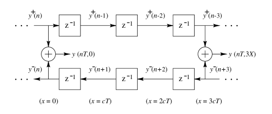
Figure 2: Digital simulation of the ideal, lossless waveguide with observation points at $x=0$ and $x=3X=3cT$. (The symbol “$z^{-1}$” denotes a one-sample delay.)

Figure 2 shows a signal flow diagram for the computational model of (6), which is often called a digital waveguide model (for the ideal string in this case) SmithPMUDW ; SmithDWMMI . Note that, by the sampling theorem, it is an exact model so long as the initial conditions and any ongoing additive excitations are bandlimited to less than half the temporal sampling rate $f_{s}=1/T$ (MDFT, , Appendix G).

Note also that the position along the string, $x_{m}=mX=mcT$ meters, is laid out from left to right in the diagram, giving a physical interpretation to the horizontal direction in the diagram, even though spatial samples have been eliminated from explicit consideration. (The arguments of $y^{+}$ and $y^{-}$ have physical units of time.)

The left- and right-going traveling wave components are summed to produce a physical output according to

$$y(nT,mX)=y^{+}(n-m)+y^{-}(n+m)$$ (7)

In Fig. 2, “transverse displacement outputs” have been arbitrarily placed at $x=0$ and $x=3X$. The diagram is similar to that of well known ladder and lattice digital filter structures MG , except for the delays along the upper rail, the absence of scattering junctions, and the direct physical interpretation.

(A scattering junction implements partial reflection and partial transmission in the waveguide.) The absence of scattering junctions is due to the fact that the string has wave impedance $R=\sqrt{K\epsilon}$ which is constant with respect to time and position. In acoustic tube simulations, such as for voice synthesis MG , lossless scattering junctions are used at changes in cross-sectional tube area and lossy scattering junctions are used to implement tone holes.

II.3 FDTD and DW Equivalence

The FDTD and DW recursions both compute time updates by forming fixed linear combinations of past state. As a result, each can be described in “state-space form” (JOSFP, , Appendix E) by a constant matrix operator, the “state transition matrix”, which multiplies the state vector at the current time to produce the state vector for the next time step. The FDTD operator propagates K variables while the DW operator propagates W variables. We may show equivalence by (1) defining a one-to-one transformation which will convert K variables to W variables or vice versa, and (2) showing that given any common initial state for both schemes, the state transition matrices compute the same next state in both cases.

The next section shows that the linear transformation from W to K variables,

$$y(n,m)=y^{+}(n-m)+y^{-}(n+m),$$ (8)

for all $n$ and $m$, sets up a one-to-one linear transformation between the K and W variables. Assuming this holds, it only remains to be shown that the DW and FDTD schemes preserve mapping (8) after a state transition from one time to the next. While this has been shown previously SmithMohonkBook98 , we repeat the derivation here for completeness. We also provide a state-space analysis reaching the same conclusion in §V.

From Fig. 2, it is clear that the DW scheme preserves mapping (8) by definition. For the FDTD scheme, we expand the right-hand of (4) using (8) and verify that the left-hand side also satisfies the map, i.e., that $y(n+1,m)=y^{+}(n+1-m)+y^{-}(n+1+m)$ holds:

$$y(n+1,m) = y(n,m+1)+y(n,m-1)-y(n-1,m)$$

$$= y^{+}(n-m-1)+y^{-}(n+m+1)$$

$$+y^{+}(n-m+1)+y^{-}(n+m-1)$$

$$-y^{+}(n-m-1)-y^{-}(n+m-1)$$

$$= y^{-}(n+m+1)+y^{+}(n-m+1)$$

$$= y^{+}[(n+1)-m]+y^{-}[(n+1)+m]$$

$$\mathrel{\stackrel{{\scriptstyle\Delta}}{{=}}} y(n+1,m)$$

Since the DW method propagates sampled (bandlimited) solutions to the ideal wave equation without error, it follows that the FDTD method does the same thing, despite the relatively crude approximations made in (3). In particular, it is known that the FDA introduces artificial damping when applied to first order partial derivatives arising in lumped, mass-spring systems SmithDWMMI .

The equivalence of the DW and FDTD state transitions extends readily to the DW mesh VanDuyneAndSmithMesh ; SmithDWMMI which is essentially a lattice-work of DWs for simulating membranes and volumes. The equivalence is more important in higher dimensions because the FDTD formulation requires less computations per node than the DW approach in higher dimensions (see BeesonEtAlDAFX04 for some quantitative comparisons).

Even in one dimension, the DW and finite-difference methods have unique advantages in particular situations MattiMohonk03 , and as a result they are often combined together to form a hybrid traveling-wave/physical-variable simulation PitteroffAndWoodhouse98b ; PitteroffAndWoodhouse98c ; Matti02 ; ErkutAndMatti02 ; ErkutAndMattiISMA02 ; MattiSMAC03 ; ArvindhAndSmithMohonk03 ; BeesonEtAlDAFX04 .

III State Transformations

In previous work, time-domain adaptors (digital filters) converting between K variables and W variables have been devised MattiMohonk03 . In this section, an alternative approach is proposed. Mapping (8) gives us an immediate conversion from W to K state variables, so all we need now is the inverse map for any time $n$. This is complicated by the fact that non-local spatial dependencies can go indefinitely in one direction along the string, as we will see below. We will proceed by first writing down the conversion from W to K variables in matrix form, which is easy to do, and then invert that matrix. For simplicity, we will consider the case of an infinitely long string.

To initialize a K variable simulation for starting at time $n+1$, we need initial spatial samples at all positions $m$ for two successive times $n-1$ and $n$. From this state specification, the FDTD scheme (4) can compute $y(n+1,m)$ for all $m$, and so on for increasing $n$. In the DW model, all state variables are defined as belonging to the same time $n$, as shown in Fig. III.

Figure 3: DW flow diagram.

From (7), and referring to the notation defined in Fig. III, we may write the conversion from W to K variables as

$$y_{n,m+1} = y^{+}_{n,m+1}+y^{-}_{n,m+1}$$

$$y_{n,m-1} = y^{+}_{n,m-1}+y^{-}_{n,m-1}$$

$$y_{n-1,m} = y^{+}_{n-1,m}+y^{-}_{n-1,m}$$ (9)

$$= y^{+}_{n,m+1}+y^{-}_{n,m-1}$$

where the last equality follows from the traveling-wave behavior (see Fig. III).

Figure 4: Stencil of the FDTD scheme.

Figure III shows the so-called “stencil” of the FDTD scheme. The larger circles indicate the state at time $n$ which can be used to compute the state at time $n+1$. The filled and unfilled circles indicate membership in one of two interleaved grids BilbaoT . To see why there are two interleaved grids, note that when $m$ is even, the update for $y_{n+1,m}$ depends only on odd $m$ from time $n$ and even $m$ from time $n-1$. Since the two W components of $y_{n-1,m}$ are converted to two W components at time $n$ in (9), we have that the update for $y_{n+1,m}$ depends only on W components from time $n$ and positions $m\pm 1$. Moving to the next position update, for $y_{n+1,m+1}$, the state used is independent of that used for $y_{n+1,m}$, and the W components used are from positions $m$ and $m+2$. As a result of these observations, we see that we may write the state-variable transformation separately for even and odd $m$, e.g.,

$$\left[\!\begin{array}[]{c}\vdots\\ y_{n,m-1}\\ y_{n-1,m}\\ y_{n,m+1}\\ y_{n-1,m+2}\\ y_{n,m+3}\\ y_{n-1,m+4}\\ y_{n,m+5}\\ \vdots\\ \end{array}\!\right]\!=\!\left[\!\begin{array}[]{cccccccccc}\ddots&&\vdots&\vdots&\vdots&\vdots&\vdots&\vdots&\vdots&0\\ \cdots&1&1&0&0&0&0&0&0&\cdots\\ \cdots&0&1&1&0&0&0&0&0&\cdots\\ \cdots&0&0&1&1&0&0&0&0&\cdots\\ \cdots&0&0&0&1&1&0&0&0&\cdots\\ \cdots&0&0&0&0&1&1&0&0&\cdots\\ \cdots&0&0&0&0&0&1&1&0&\cdots\\ \cdots&0&0&0&0&0&0&1&1&\cdots\\ 0&\vdots&\vdots&\vdots&\vdots&\vdots&\vdots&\vdots&\ddots\end{array}\!\right]\left[\!\begin{array}[]{c}\vdots\\ y^{+}_{n,m-1}\\ y^{-}_{n,m-1}\\ y^{+}_{n,m+1}\\ y^{-}_{n,m+1}\\ y^{+}_{n,m+3}\\ y^{-}_{n,m+3}\\ y^{+}_{n,m+5}\\ y^{-}_{n,m+5}\\ \vdots\end{array}\!\right].$$ (10)

Denote the linear transformation operator by $\mathbf{T}$ and the K and W state vectors by $\underline{x}_{K}$ and $\underline{x}_{W}$, respectively. Then (10) can be restated as

$$\underline{x}_{K}=\mathbf{T}\underline{x}_{W}.$$ (11)

The operator $\mathbf{T}$ can be recognized as the Toeplitz operator associated with the linear, shift-invariant filter $H(z)=1+z^{-1}$. While the present context is not a simple convolution since $\underline{x}_{W}$ is not a simple time series, the inverse of $\mathbf{T}$ corresponds to the Toeplitz operator associated with

$$H(z)=\frac{1}{1+z^{-1}}=1-z^{-1}+z^{-2}-z^{-3}+\cdots.$$

Therefore, we may easily write down the inverted transformation:

$$\left[\!\begin{array}[]{c}\vdots\\ y^{+}_{n,m-1}\\ y^{-}_{n,m-1}\\ y^{+}_{n,m+1}\\ y^{-}_{n,m+1}\\ y^{+}_{n,m+3}\\ y^{-}_{n,m+3}\\ y^{+}_{n,m+5}\\ y^{-}_{n,m+5}\\ \vdots\end{array}\!\right]\!=\!\left[\!\begin{array}[]{crrrrrrrrc}\ddots&&\vdots&\vdots&\vdots&\vdots&\vdots&\vdots&\vdots&\pm 1\\ \cdots&1&-1&1&-1&1&-1&1&-1&\cdots\\ \cdots&0&1&-1&1&-1&1&-1&1&\cdots\\ \cdots&0&0&1&-1&1&-1&1&-1&\cdots\\ \cdots&0&0&0&1&-1&1&-1&1&\cdots\\ \cdots&0&0&0&0&1&-1&1&-1&\cdots\\ \cdots&0&0&0&0&0&1&-1&1&\cdots\\ \cdots&0&0&0&0&0&0&1&-1&\cdots\\ 0&\vdots&\vdots&\vdots&\vdots&\vdots&\vdots&\vdots&\ddots\end{array}\!\right]\left[\!\begin{array}[]{c}\vdots\\ y_{n,m-1}\\ y_{n-1,m}\\ y_{n,m+1}\\ y_{n-1,m+2}\\ y_{n,m+3}\\ y_{n-1,m+4}\\ y_{n,m+5}\\ \vdots\\ \end{array}\!\right]$$ (12)

The case of the finite string is identical to that of the infinite string when the matrix $\mathbf{T}$ is simply “cropped” to a finite square size (leaving an isolated 1 in the lower right corner); in such cases, $\mathbf{T}^{-1}$ as given above is simply cropped to the same size, retaining its upper triangular $\pm 1$ structure. Another interesting set of cases is obtained by inserting a 1 in the lower-left corner of the cropped $\mathbf{T}$ matrix to make it circulant; in these cases, the $M\times M$ matrix $\mathbf{T}^{-1}$ contains $\pm 1/2$ in every position for even $M$, and is singular for odd $M$ (when there is one zero eigenvalue).

IV Examples

IV.1 Localized Displacement Excitations

Whenever two adjacent components of $\underline{x}_{K}$ are initialized with equal amplitude, only a single $W$-variable will be affected. For example, the initial conditions (for time $n+1$)

$$y_{n,m-1} = 1$$

$$y_{n-1,m} = 1$$

will initialize only $y^{-}_{n,m-1}$, a solitary left-going pulse of amplitude 1 at time $n=0$, as can be seen from (12) by adding the leftmost columns explicitly written for $\mathbf{T}^{-1}$. Similarly, the initialization

$$y_{n-1,m-2} = 1$$

$$y_{n,m-1} = 1$$

gives rise to an isolated right-going pulse $y^{+}_{n,m-1}$, corresponding to the leftmost column of $\mathbf{T}^{-1}$ plus the first column on the left not explicitly written in (12). The superposition of these two examples corresponds to a physical impulsive excitation at time 0 and position $m-1$:

$$y_{n-1,m-2} = 1$$

$$y_{n,m-1} = 2$$

$$y_{n-1,m} = 1$$ (13)

Thus, the impulse starts out with amplitude 2 at time 0 and position $m-1$, and afterwards, impulses of amplitude 1 propagate away to the left and right along the string.

In summary, we see that to excite a single sample of displacement traveling in a single-direction, we must excite equally a pair of adjacent colums in $\mathbf{T}^{-1}$. This corresponds to equally weighted excitation of K-variable pairs the form $(y_{n,m},y_{n-1,m\pm 1})$.

Note that these examples involved only one of the two interleaved computational grids. Shifting over an odd number of spatial samples to the left or right would involve the other grid, as would shifting time forward or backward an odd number of samples.

IV.2 Localized Velocity Excitations

Initial velocity excitations are straightforward in the DW paradigm, but can be less intuitive in the FDTD domain. It is well known that velocity in a displacement-wave DW simulation is determined by the difference of the right- and left-going waves SmithPMUDW . Specifically, initial velocity waves $v^{\pm}$ can be computed from from initial displacement waves $y^{\pm}$ by spatially differentiating $y^{\pm}$ to obtain traveling slope waves $y^{\prime\pm}$, multiplying by minus the tension $K$ to obtain force waves, and finally dividing by the wave impedance $R=\sqrt{K\epsilon}$ to obtain velocity waves:

$$v^{+} = -cy^{\prime{+}}=\frac{f^{+}}{R}$$

$$v^{-} = \;cy^{\prime{-}}=-\frac{f^{-}}{R},$$ (14)

where $c=\sqrt{K/\epsilon}$ denotes sound speed. The initial string velocity at each point is then $v(nT,mX)=v^{+}(n-m)+v^{-}(n+m)$. (A more direct derivation can be based on differentiating (5) with respect to $x$ and solving for velocity traveling-wave components, considering left- and right-going cases separately at first, and arguing the general case by superposition.)

We can see from (12) that such asymmetry can be caused by unequal weighting of $y_{n,m}$ and $y_{n,m\pm 1}$. For example, the initialization

$$y_{n-1,m+1} = +1$$

$$y_{n-1,m} = -1$$

corresponds to an impulse velocity excitation at position $m+1/2$. In this case, both interleaved grids are excited.

IV.3 More General Velocity Excitations

From (12), it is clear that initializing any single K variable $y_{n,m}$ corresponds to the initialization of an infinite number of W variables $y^{+}_{n,m}$ and $y^{-}_{n,m}$. That is, a single K variable $y_{n,m}$ corresponds to only a single column of $\mathbf{T}^{-1}$ for only one of the interleaved grids. For example, referring to (12), initializing the K variable $y_{n-1,m}$ to -1 at time $n$ (with all other $y_{n,m}$ intialized to 0) corresponds to the W-variable initialization

$$y^{+}_{n,m-(2\mu+1)} = +1,\quad\mu=0,1,2,\cdots$$

$$y^{-}_{n,m-(2\mu+1)} = -1,\quad\mu=0,1,2,\cdots$$

with all other W variables being initialized to zero. In view of earlier remarks, this corresponds to an impulsive velocity excitation on only one of the two subgrids. A schematic depiction from $\mu=m-5$ to $m+5$ of the W variables at time $n$ is as follows:

$$\begin{array}[]{crrrrr|rrrrrrc}\cdots&1&0&1&0&1&0&0&0&0&0&0&\cdots\\ \cdots&-1&0&-1&0&-1&0&0&0&0&0&0&\cdots\\ \hline\cr\\[-10.00002pt] \cdots&0&0&0&0&0&0&0&0&0&0&0&\cdots\\ &&&&&&m&&&&&\mu&\rightarrow\end{array}$$ (15)

Below the solid line is the sum of the left- and right-going traveling-wave components, i.e., the corresponding K variables at time $n$. The vertical lines divide positions $\mu=m-1$ and $\mu=m$. The initial displacement is zero everywhere at time $n$, consistent with an initial velocity excitation. At times $\nu=n+1,n+2,n+3,n+4$, the configuration evolves as follows:

$$\begin{array}[]{crrrrr|rrrrrrc}\cdots&0&1&0&1&0&1&0&0&0&0&0&\cdots\\ \cdots&0&-1&0&-1&0&0&0&0&0&0&0&\cdots\\ \hline\cr\\[-10.00002pt] \cdots&0&0&0&0&0&1&0&0&0&0&0&\cdots\end{array}$$ (16)

$$\begin{array}[]{crrrrr|rrrrrrc}\cdots&1&0&1&0&1&0&1&0&0&0&0&\cdots\\ \cdots&-1&0&-1&0&0&0&0&0&0&0&0&\cdots\\ \hline\cr\\[-10.00002pt] \cdots&0&0&0&0&1&0&1&0&0&0&0&\cdots\end{array}$$ (17)

$$\begin{array}[]{crrrrr|rrrrrrc}\cdots&0&1&0&1&0&1&0&1&0&0&0&\cdots\\ \cdots&0&-1&0&0&0&0&0&0&0&0&0&\cdots\\ \hline\cr\\[-10.00002pt] \cdots&0&0&0&1&0&1&0&1&0&0&0&\cdots\end{array}$$ (18)

$$\begin{array}[]{crrrrr|rrrrrrc}\cdots&1&0&1&0&1&0&1&0&1&0&0&\cdots\\ \cdots&-1&0&0&0&0&0&0&0&0&0&0&\cdots\\ \hline\cr\\[-10.00002pt] \cdots&0&0&1&0&1&0&1&0&1&0&0&\cdots\end{array}$$ (19)

The sequence $[\dots,1,0,1,0,1,\dots]$ consists of a dc (zero-frequency) component with amplitude $1/2$, plus a sampled sinusoid of amplitude $1/2$ oscillating at half the sampling rate $f_{s}=1/T$. The dc component is physically correct for an initial velocity point-excitation (a spreading square pulse on the string is expected). However, the component at $f_{s}/2$ is usually regarded as an artifact of the finite difference scheme. From the DW interpretation of the FDTD scheme, which is an exact, bandlimited physical interpretation, we see that physically the component at $f_{s}/2$ comes about from initializing velocity on only one of the two interleaved subgrids of the FDTD scheme. Any asymmetry in the excitation of the two interleaved grids will result in excitation of this frequency component.

Due to the independent interleaved subgrids in the FDTD algorithm, it is nearly always non-physical to excite only one of them, as the above example makes clear. It is analogous to illuminating only every other pixel in a digital image. However, joint excitation of both grids may be accomplished either by exciting adjacent spatial samples at the same time, or the same spatial sample at successive times instants.

In addition to the W components being non-local, they can demand a larger dynamic range than the K variables. For example, if the entire semi-infinite string for $m<0$ is initialized with velocity $2X/T$, the initial displacement traveling-wave components look as follows:

$$\begin{array}[]{crrrrrr|rrrrrc}\cdots&6&5&4&3&2&1&0&0&0&0&0&\cdots\\ \cdots&-6&-5&-4&-3&-2&-1&0&0&0&0&0&\cdots\\ \hline\cr\\[-10.00002pt] \cdots&0&0&0&0&0&0&0&0&0&0&0&\cdots\end{array}$$ (20)

and the variables evolve forward in time as follows:

$$\begin{array}[]{crrrrrr|rrrrrc}\cdots&7&6&5&4&3&2&1&0&0&0&0&\cdots\\ \cdots&-5&-4&-3&-2&-1&0&0&0&0&0&0&\cdots\\ \hline\cr\\[-10.00002pt] \cdots&2&2&2&2&2&2&1&0&0&0&0&\cdots\end{array}$$ (21)

$$\begin{array}[]{crrrrrr|rrrrrc}\cdots&8&7&6&5&4&3&2&1&0&0&0&\cdots\\ \cdots&-4&-3&-2&-1&0&0&0&0&0&0&0&\cdots\\ \hline\cr\\[-10.00002pt] \cdots&4&4&4&4&4&3&2&1&0&0&0&\cdots\end{array}$$ (22)

$$\begin{array}[]{crrrrrr|rrrrrc}\cdots&9&8&7&6&5&4&3&2&1&0&0&\cdots\\ \cdots&-3&-2&-1&0&0&0&0&0&0&0&0&\cdots\\ \hline\cr\\[-10.00002pt] \cdots&6&6&6&6&5&4&3&2&1&0&0&\cdots\end{array}$$ (23)

Thus, the left semi-infinite string moves upward at a constant velocity of 2, while a ramp spreads out to the left and right of position $\mu=m$ at speed $c$, as expected physically. By (10), the corresponding initial FDTD state for this case is

$$y_{n,\mu} = 0,\quad\mu\in{\bf Z}$$

$$y_{n-1,m-1} = -1,$$

$$y_{n-1,\mu} = -2,\quad\mu<m-1,$$

where ${\bf Z}$ denotes the set of all integers. While the FDTD excitation is also not local, of course, it is bounded for all $\mu$.

Since the traveling-wave components of initial velocity excitations are generally non-local in a displacement-based simulation, as illustrated in the preceding examples, it is often preferable to use velocity waves (or force waves) in the first place SmithDWMMI .

Another reason to prefer force or velocity waves is that displacement inputs are inherently impulsive. To see why this is so, consider that any physically correct driving input must effectively exert some finite force on the string, and this force is free to change arbitrarily over time. The “equivalent circuit” of the infinitely long string at the driving point is a “dashpot” having real, positive resistance $2R=2\sqrt{K\epsilon}$. The applied force $f(t)$ can be divided by $2R$ to obtain the velocity $v(t)$ of the string driving point, and this velocity is free to vary arbitrarily over time, proportional to the applied force. However, this velocity must be time-integrated to obtain a displacement $y(t)$. Therefore, there can be no instantaneous displacement response to a finite driving force. In other words, any instantaneous effect of an input driving signal on an output displacement sample is non-physical except in the case of a massless system. Infinite force is required to move the string instantaneously. In sampled displacement simulations, we must interpret displacement changes as resulting from time-integration over a sampling period. As the sampling rate increases, any physically meaningful displacement driving signal must converge to zero.

IV.4 Additive Inputs

Instead of initial conditions, ongoing input signals can be defined analogously. For example, feeding an input signal $u_{n}$ into the FDTD via

$$y_{n,m-1} = y_{n,m-1}+u_{n-1}$$

$$y_{n,m} = y_{n,m}+2u_{n}$$

$$y_{n,m+1} = y_{n,m+1}+u_{n-1}$$ (24)

corresponds to physically driving a single sample of string displacement at position $m$. This is the spatially distributed alternative to the temporally distributed solution of feeding an input to a single displacement sample via the filter $H(z)=1-z^{-2}$ as discussed in MattiMohonk03 .

IV.5 Physical Interpretation of $H(z)=1-z^{-2}$

As shown above, driving a single displacement sample $y_{n,m}$ in the FDTD corresponds to driving a velocity input at position $m$ on two alternating subgrids over time. Therefore, the filter $H(z)=1-z^{-2}$ acts as the filter $H(z)=1-z^{-1}$ on either subgrid alone—a first-order difference. Since displacement is being simulated, velocity inputs must be numerically integrated. The first-order difference can be seen as canceling this integration, thereby converting a velocity input to a displacement input, as in (24).

V State Space Formulation

In this section, we will summarize and extend the above discussion by means of a state space analysis Kailath80 .

V.1 FDTD State Space Model

Let $\underline{x}_{K}(n)$ denote the FDTD state for one of the two subgrids at time $n$, as defined by (11). The other subgrid is handled identically and will not be considered explicitly. In fact, the other subgrid can be dropped altogether to obtain a half-rate, staggered grid scheme BilbaoT ; Fornberg98 . However, boundary conditions and input signals will couple the subgrids, in general. To land on the same subgrid after a state update, it is necessary to advance time by two samples instead of one. The state-space model for one subgrid of the FDTD model of the ideal string may then be written as

$$\underline{x}_{K}(n+2) = \mathbf{A}_{K}\,\underline{x}_{K}(n)+\mathbf{B}_{K}\,\underline{u}(n+2)$$

$$\underline{y}(n) = \mathbf{C}_{K}\,\underline{x}_{K}(n).$$ (25)

To avoid the issue of boundary conditions for now, we will continue working with the infinitely long string. As a result, the state vector $\underline{x}_{K}(n)$ denotes a point in a space of countably infinite dimensionality. A proper treatment of this case would be in terms of operator theory NaylorAndSell82 . However, matrix notation is also clear and will be used below. Boundary conditions are taken up in §V.3.

When there is a general input signal vector $\underline{u}(n)$, it is necessary to augment the input matrix $\mathbf{B}_{K}$ to accomodate contributions over both time steps. This is because inputs to positions $m\pm 1$ at time $n+1$ affect position $m$ at time $n+2$. Henceforth, we assume $\mathbf{B}_{K}$ and $\underline{u}$ have been augmented in this way. Thus, if there are $q$ input signals $\underline{\upsilon}(n)\buildrel\scriptscriptstyle\Delta\over{\scriptstyle=}[\upsilon_{i}(n)]$, $i=1,\ldots,q$, driving the full string state through weights $\underline{\beta}_{m}\buildrel\scriptscriptstyle\Delta\over{\scriptstyle=}[\beta_{m,i}]$, $m\in{\bf Z}$, the vector $\underline{u}(n)=$ is of dimension $2q\times 1$:

$$\underline{u}(n+2)=\left[\!\begin{array}[]{c}\underline{\upsilon}(n+2)\\ \underline{\upsilon}(n+1)\end{array}\!\right]$$

When there is only one physical input, as is typically assumed for plucked, struck, and bowed strings, then $q=1$ and $\underline{u}$ is $2\times 1$. The matrix $\mathbf{B}_{K}$ weights these inputs before they are added to the state vector for time $n+2$, and its entries are derived in terms of the $\beta_{m,i}$ coefficients below.

$\mathbf{C}_{K}$ forms the output signal as an arbitrary linear combination of states. To obtain the usual displacement output for the subgrid, $\mathbf{C}_{K}$ is the matrix formed from the identity matrix by deleting every other row, thereby retaining all displacement samples at time $n$ and discarding all displacement samples at time $n-1$ in the state vector $\underline{x}_{K}(n)$:

$$\underbrace{\left[\!\begin{array}[]{c}\vdots\\ y_{n,m-2}\\ y_{n,m}\\ y_{n,m+2}\\ y_{n,m+4}\\ \vdots\end{array}\!\right]}_{\underline{y}(n)}\!=\!\underbrace{\left[\!\begin{array}[]{ccccccccccc}&\vdots&\vdots&\vdots&\vdots&\vdots&\vdots&\vdots&\vdots\\ \cdots&1&0&0&0&0&0&0&0&\cdots\\ \cdots&0&0&1&0&0&0&0&0&\cdots\\ \cdots&0&0&0&0&1&0&0&0&\cdots\\ \cdots&0&0&0&0&0&0&1&0&\cdots\\ &\vdots&\vdots&\vdots&\vdots&\vdots&\vdots&\vdots&\vdots\end{array}\!\right]}_{\mathbf{C}_{K}}\underbrace{\left[\!\begin{array}[]{c}\vdots\\ y_{n,m-2}\\ y_{n-1,m-1}\\ y_{n,m}\\ y_{n-1,m+1}\\ y_{n,m+2}\\ y_{n-1,m+3}\\ y_{n,m+4}\\ \vdots\end{array}\!\right]}_{\underline{x}_{K}(n)}$$

The state transition matrix $\mathbf{A}_{K}$ may be obtained by first performing a one-step time update,

$$y_{n+2,m}=y_{n+1,m-1}+y_{n+1,m+1}-y_{n,m}+\underline{\beta}_{m}^{T}\underline{\upsilon}(n+2),$$

and then expanding the two $n+1$ terms in terms of the state at time $n$:

$$y_{n+1,m-1} = y_{n,m-2}+y_{n,m}-y_{n-1,m-1}+\underline{\beta}_{m-1}^{T}\underline{\upsilon}(n+1)$$

$$y_{n+1,m+1} = y_{n,m}+y_{n,m+2}-y_{n-1,m+1}+\underline{\beta}_{m+1}^{T}\underline{\upsilon}(n+1)$$

The intra-grid state update for even $m$ is then given by

$$y_{n+2,m}$$ (38)

$$= y_{n,m-2}-y_{n-1,m-1}+y_{n,m}-y_{n-1,m+1}+y_{n,m+2}$$

$$\quad+\;\underline{\beta}_{m}^{T}\underline{\upsilon}(n+2)+(\underline{\beta}_{m-1}+\underline{\beta}_{m+1})^{T}\underline{\upsilon}(n+1)$$

$$= \begin{array}[]{c}\left[1,-1,1,-1,1\right]\\ \vspace{0.5in}\hfil\end{array}\left[\!\begin{array}[]{l}y_{n,m-2}\\ y_{n-1,m-1}\\ y_{n,m}\\ y_{n-1,m+1}\\ y_{n,m+2}\\ y_{n-1,m+3}\\ \end{array}\!\right]$$

$$+\left[\underline{\beta}_{m}^{T}\quad(\underline{\beta}_{m-1}+\underline{\beta}_{m+1})^{T}\right]\left[\!\begin{array}[]{l}\underline{\upsilon}(n+2)\\ \underline{\upsilon}(n+1)\end{array}\!\right].$$

For odd $m$, the update in (LABEL:eq:oddm) is used. Thus, every other row of $\mathbf{A}_{K}$, for time $n+2$, consists of the vector $[1,-1,1,-1,1]$ preceded and followed by zeros. Successive rows for time $n+2$ are shifted right two places. The rows for time $n+1$ consist of the vector $[1,-1,1]$ aligned similarly:

$$\underbrace{\left[\!\begin{array}[]{l}\qquad\vdots\\ y_{n+1,m-1}\\ y_{n+2,m}\\ y_{n+1,m+1}\\ y_{n+2,m+2}\\ \qquad\vdots\end{array}\!\right]}_{\underline{x}_{K}(n+2)}\!\leftarrow\!\underbrace{\left[\!\begin{array}[]{rrrrrrrrrrr}&\vdots&\vdots&\vdots&\vdots&\vdots&\vdots&\vdots\\ \cdots&1&-1&1&0&0&0&0&\cdots\\ \cdots&1&-1&1&-1&1&0&0&\cdots\\ \cdots&0&0&1&-1&1&0&0&\cdots\\ \cdots&0&0&1&-1&1&-1&1&\cdots\\ &\vdots&\vdots&\vdots&\vdots&\vdots&\vdots&\vdots\end{array}\!\right]}_{\mathbf{A}_{K}}\!\underbrace{\left[\!\begin{array}[]{l}\qquad\vdots\\ y_{n,m-2}\\ y_{n-1,m-1}\\ y_{n,m}\\ y_{n-1,m+1}\\ y_{n,m+2}\\ y_{n-1,m+3}\\ \qquad\vdots\end{array}\!\right]}_{\underline{x}_{K}(n)}$$

From (38) we also see that the input matrix $\mathbf{B}_{K}$ is given as defined in the following expression:

$$\underbrace{\left[\!\begin{array}[]{l}\qquad\vdots\\ y_{n+1,m-1}\\ y_{n+2,m}\\ y_{n+1,m+1}\\ y_{n+2,m+2}\\ y_{n+1,m+3}\\ y_{n+2,m+4}\\ y_{n+1,m+5}\\ \qquad\vdots\end{array}\!\right]}_{\underline{x}_{K}(n+2)}\leftarrow\underbrace{\left[\!\begin{array}[]{cc}\vdots&\vdots\\ 0&\underline{\beta}_{m-1}^{T}\\[5.0pt] \underline{\beta}_{m}^{T}&\quad\underline{\beta}_{m-1}^{T}+\underline{\beta}_{m+1}^{T}\\[5.0pt] 0&\underline{\beta}_{m+1}^{T}\\[5.0pt] \underline{\beta}_{m+2}^{T}&\underline{\beta}_{m+1}^{T}+\underline{\beta}_{m+3}^{T}\\[5.0pt] 0&\underline{\beta}_{m+3}^{T}\\[5.0pt] \underline{\beta}_{m+4}^{T}&\underline{\beta}_{m+3}^{T}+\underline{\beta}_{m+5}^{T}\\[5.0pt] 0&\underline{\beta}_{m+5}^{T}\\[5.0pt] \vdots&\vdots\end{array}\!\right]}_{\mathbf{B}_{K}}\underbrace{\left[\!\begin{array}[]{c}\underline{\upsilon}(n+2)\\ \underline{\upsilon}(n+1)\end{array}\!\right]}_{\underline{u}(n+2)}.$$

V.2 DW State Space Model

As discussed in §III, the traveling-wave decomposition (5) defines a linear transformation (11) from the DW state to the FDTD state:

$$\underline{x}_{K}=\mathbf{T}\,\underline{x}_{W}$$ (39)

Since $\mathbf{T}$ is invertible, it qualifies as a linear transformation for performing a change of coordinates for the state space. Substituting (39) into the FDTD state space model (25) gives

$$\mathbf{T}\,\underline{x}_{W}(n+2) = \mathbf{A}_{K}\,\mathbf{T}\,\underline{x}_{W}(n)+\mathbf{B}_{K}\,\underline{u}(n+2)$$ (40)

$$\underline{y}(n) = \mathbf{C}_{K}\,\mathbf{T}\,\underline{x}_{W}(n).$$ (41)

Multiplying through (40) by $\mathbf{T}^{-1}$ gives a new state-space representation of the same dynamic system which we will show is in fact the DW model of Fig. III:

$$\underline{x}_{W}(n+2) = \mathbf{A}_{W}\,\underline{x}_{W}(n)+{\mathbf{B}_{W}}\,\underline{u}(n+2)$$

$$\underline{y}(n) = \mathbf{C}_{W}\,\underline{x}_{W}(n)$$ (42)

where

$$\mathbf{A}_{W} \mathrel{\stackrel{{\scriptstyle\Delta}}{{=}}} \mathbf{T}^{-1}\mathbf{A}_{K}\,\mathbf{T}$$

$${\mathbf{B}_{W}} \mathrel{\stackrel{{\scriptstyle\Delta}}{{=}}} \mathbf{T}^{-1}\mathbf{B}_{K}$$

$$\mathbf{C}_{W} \mathrel{\stackrel{{\scriptstyle\Delta}}{{=}}} \mathbf{C}_{K}\,\mathbf{T}$$ (43)

To verify that the DW model derived in this manner is the computation diagrammed in Fig. III, we may write down the state transition matrix for one subgrid from the figure to obtain the permutation matrix $\mathbf{A}_{W}$,

$$\underbrace{\left[\!\begin{array}[]{l}\qquad\vdots\\ y^{+}_{n+2,m-2}\\ y^{-}_{n+2,m-2}\\ y^{+}_{n+2,m}\\ y^{-}_{n+2,m}\\ y^{+}_{n+2,m+2}\\ y^{-}_{n+2,m+2}\\ \qquad\vdots\end{array}\!\right]}_{\underline{x}_{W}(n+2)}\!\leftarrow\!\underbrace{\left[\!\begin{array}[]{cccccccccccc}\cdots&\vdots&\vdots&\vdots&\vdots&\vdots&\vdots&\vdots&\vdots&\vdots&\vdots\\ \cdots&1&0&0&0&0&0&0&0&0&0&\cdots\\ \cdots&0&0&0&0&0&1&0&0&0&0&\cdots\\ \cdots&0&0&1&0&0&0&0&0&0&0&\cdots\\ \cdots&0&0&0&0&0&0&0&1&0&0&\cdots\\ \cdots&0&0&0&0&1&0&0&0&0&0&\cdots\\ \cdots&0&0&0&0&0&0&0&0&0&1&\cdots\\ \cdots&\vdots&\vdots&\vdots&\vdots&\vdots&\vdots&\vdots&\vdots&\vdots&\vdots\end{array}\!\right]}_{\mathbf{A}_{W}}\!\underbrace{\left[\!\begin{array}[]{l}\quad\vdots\\ y^{+}_{n,m-4}\\ y^{-}_{n,m-4}\\ y^{+}_{n,m-2}\\ y^{-}_{n,m-2}\\ y^{+}_{n,m}\\ y^{-}_{n,m}\\ y^{+}_{n,m+2}\\ y^{-}_{n,m+2}\\ y^{+}_{n,m+4}\\ y^{-}_{n,m+4}\\ \quad\vdots\end{array}\!\right]}_{\underline{x}_{W}(n)}$$ (44)

and displacement output matrix $\mathbf{C}_{W}$:

$$\underbrace{\left[\!\begin{array}[]{c}\vdots\\ y_{n,m-2}\\ y_{n,m}\\ y_{n,m+2}\\ y_{n,m+4}\\ \vdots\end{array}\!\right]}_{\underline{y}(n)}=\underbrace{\left[\!\begin{array}[]{cccccccccc}&\vdots&\vdots&\vdots&\vdots&\vdots&\vdots&\vdots&\vdots&\\ \cdots&1&1&0&0&0&0&0&0&\cdots\\ \cdots&0&0&1&1&0&0&0&0&\cdots\\ \cdots&0&0&0&0&1&1&0&0&\cdots\\ \cdots&0&0&0&0&0&0&1&1&\cdots\\ &\vdots&\vdots&\vdots&\vdots&\vdots&\vdots&\vdots&\vdots&\end{array}\!\right]}_{\mathbf{C}_{W}}\underbrace{\left[\!\begin{array}[]{l}\quad\vdots\\ y^{+}_{n,m-2}\\ y^{-}_{n,m-2}\\ y^{+}_{n,m}\\ y^{-}_{n,m}\\ y^{+}_{n,m+2}\\ y^{-}_{n,m+2}\\ y^{+}_{n,m+4}\\ y^{-}_{n,m+4}\\ \quad\vdots\end{array}\!\right]}_{\underline{x}_{W}(n)}$$

V.2.1 DW Displacement Inputs

We define general DW inputs as follows:

$$y^{+}_{n,m} = y^{+}_{n-1,m-1}+(\underline{\gamma}^{+}_{m})^{T}\underline{\upsilon}(n)$$ (45)

$$y^{-}_{n,m} = y^{-}_{n-1,m+1}+(\underline{\gamma}^{-}_{m})^{T}\underline{\upsilon}(n)$$ (46)

The $m$th $2q\times 2$ block of the input matrix ${\mathbf{B}_{W}}$ driving state components $[y^{+}_{n+2,m},y^{-}_{n+2,m}]^{T}$ and multiplying $[\underline{\upsilon}(n+2)^{T},\underline{\upsilon}(n+1)^{T}]^{T}$ is then given by

$$\left({\mathbf{B}_{W}}\right)_{m}=\left[\!\begin{array}[]{cc}(\underline{\gamma}^{+}_{m})^{T}&(\underline{\gamma}^{+}_{m-1})^{T}\\[5.0pt] (\underline{\gamma}^{-}_{m})^{T}&(\underline{\gamma}^{-}_{m+1})^{T}\end{array}\!\right].$$ (47)

Typically, input signals are injected equally to the left and right along the string, in which case

$$\underline{\gamma}^{+}_{m}=\underline{\gamma}^{-}_{m}\mathrel{\stackrel{{\scriptstyle\Delta}}{{=}}}\underline{\gamma}_{m}.$$

Physically, this corresponds to applied forces at a single, non-moving, string position over time. The state update with this simplification appears as

$$\underbrace{\left[\!\begin{array}[]{c}\vdots\\ y^{+}_{n+2,m}\\[5.0pt] y^{-}_{n+2,m}\\ \vdots\end{array}\!\right]}_{\underline{x}_{W}(n+2)}=\mathbf{A}_{W}\underline{x}_{W}(n)+\underbrace{\left[\!\begin{array}[]{cc}\vdots&\vdots\\ \underline{\gamma}_{m}^{T}&\underline{\gamma}_{m-1}^{T}\\[5.0pt] \underline{\gamma}_{m}^{T}&\underline{\gamma}_{m+1}^{T}\\[5.0pt] \vdots&\vdots\end{array}\!\right]}_{{\mathbf{B}_{W}}}\underbrace{\left[\!\begin{array}[]{c}\underline{\upsilon}(n+2)\\ \underline{\upsilon}(n+1)\end{array}\!\right]}_{\underline{u}(n+2)}.$$

Note that if there are no inputs driving the adjacent subgrid ($\underline{\gamma}_{m-1}=\underline{\gamma}_{m+1}=0$), such as in a half-rate staggered grid scheme, the input reduces to

$$\underline{x}_{W}(n+2)=\mathbf{A}_{W}\underline{x}_{W}(n)+\underbrace{\left[\!\begin{array}[]{c}\vdots\\ \underline{\gamma}_{m-2}^{T}\\[5.0pt] \underline{\gamma}_{m-2}^{T}\\[5.0pt] \underline{\gamma}_{m}^{T}\\[5.0pt] \underline{\gamma}_{m}^{T}\\[5.0pt] \underline{\gamma}_{m+2}^{T}\\[5.0pt] \underline{\gamma}_{m+2}^{T}\\[5.0pt] \vdots\end{array}\!\right]}_{{\mathbf{B}_{W}}}\underline{\upsilon}(n+2).$$

To show that the directly obtained FDTD and DW state-space models correspond to the same dynamic system, it remains to verify that $\mathbf{A}_{W}=\mathbf{T}^{-1}\mathbf{A}_{K}\,\mathbf{T}$. It is somewhat easier to show that

$$\mathbf{T}\,\mathbf{A}_{W} = \mathbf{A}_{K}\,\mathbf{T}$$

$$= \left[\!\begin{array}[]{cccccccccccc}&\vdots&\vdots&\vdots&\vdots&\vdots&\vdots&\vdots&\vdots&\vdots&\vdots\\ \cdots&1&0&0&0&0&1&0&0&0&0&\cdots\\ \cdots&0&0&1&0&0&1&0&0&0&0&\cdots\\ \cdots&0&0&1&0&0&0&0&1&0&0&\cdots\\ \cdots&0&0&0&0&1&0&0&1&0&0&\cdots\\ &\vdots&\vdots&\vdots&\vdots&\vdots&\vdots&\vdots&\vdots&\vdots&\vdots\end{array}\!\right].$$

A straightforward calculation verifies that the above identity holds, as expected. One can similarly verify $\mathbf{C}_{W}=\mathbf{C}_{K}\,\mathbf{T}$, as expected. The relation ${\mathbf{B}_{W}}=\mathbf{T}^{-1}\,\mathbf{B}_{K}$ provides a recipe for translating any choice of input signals for the FDTD model to equivalent inputs for the DW model, or vice versa. For example, in the scalar input case ($q=1$), the DW input-weights ${\mathbf{B}_{W}}$ become FDTD input-weights $\mathbf{B}_{K}$ according to

$$\left[\!\begin{array}[]{l}\qquad\vdots\\ y_{n+1,m-1}\\ y_{n+2,m}\\ y_{n+1,m+1}\\ y_{n+2,m+2}\\ \qquad\vdots\end{array}\!\right]\!\leftarrow\!\underbrace{\left[\!\begin{array}[]{cc}\vdots&\vdots\\ \gamma^{+}_{m}+\gamma^{-}_{m-1}&\,\gamma^{+}_{m-1}+\gamma^{-}_{m-1}\\[5.0pt] \gamma^{+}_{m}+\gamma^{-}_{m}&\,\gamma^{+}_{m-1}+\gamma^{-}_{m+1}\\[5.0pt] \gamma^{-}_{m}+\gamma^{+}_{m+1}&\,\gamma^{+}_{m+1}\gamma^{-}_{m+1}\\[5.0pt] \gamma^{+}_{m+2}+\gamma^{-}_{m+2}&\,\gamma^{+}_{m+1}+\gamma^{-}_{m+3}\\[5.0pt] \vdots&\vdots\end{array}\!\right]}_{\mathbf{B}_{K}}\!\left[\!\begin{array}[]{c}\underline{\upsilon}(n+2)\\ \underline{\upsilon}(n+1)\end{array}\!\right]$$

The left- and right-going input-weight superscripts indicate the origin of each coefficient. Setting $\gamma^{+}_{m}=\gamma^{-}_{m}$ results in

$$\mathbf{B}_{K}=\left[\!\begin{array}[]{cc}\vdots&\vdots\\ \gamma_{m}+\gamma_{m-1}&\,2\gamma_{m-1}\\[5.0pt] 2\gamma_{m}&\,\gamma_{m-1}+\gamma_{m+1}\\[5.0pt] \gamma_{m}+\gamma_{m+1}&\,2\gamma_{m+1}\\[5.0pt] 2\gamma_{m+2}&\,\gamma_{m+1}+\gamma_{m+3}\\[5.0pt] \vdots&\vdots\end{array}\!\right]$$ (49)

Finally, when $\gamma_{m}=1$ and $\gamma_{\mu}=0$ for all $\mu\neq m$, we obtain the result familiar from (24):

$$\mathbf{B}_{K}=\left[\!\begin{array}[]{cc}\vdots&\vdots\\ 0&1\\ 2&0\\ 0&1\\ \vdots&\vdots\end{array}\!\right]$$

Similarly, setting $\gamma^{\pm}_{\mu}=0$ for all $\mu\neq m+1$, the weighting pattern $(1,2,1)$ appears in the second column, shifted down one row. Thus, $\mathbf{B}_{K}$ in general (for physically stationary displacement inputs) can be seen as the superposition of weight patterns $(1,2,1)$ in the left column for even $m$, and the right column for odd $m$ (the other subgrid), where the $2$ is aligned with the driven sample. This is the general collection of displacement inputs.

V.2.2 DW Non-Displacement Inputs

Since a displacement input at position $m$ corresponds to symmetrically exciting the right- and left-going traveling-wave components $y^{+}_{m}$ and $y^{-}_{m}$, it is of interest to understand what it means to excite these components antisymmetrically. As discussed in §IV.3, an antisymmetric excitation of traveling-wave components can be interpreted as a velocity excitation. It was noted that localized velocity excitations in the FDTD generally correspond to non-localized velocity excitations in the DW, and that velocity in the DW is proportional to the spatial derivative of the difference between the left-going and right-going traveling displacement-wave components (see (14)). More generally, the antisymmetric component of displacement-wave excitation can be expressed in terms of any wave variable which is linearly independent relative to displacement, such as acceleration, slope, force, momentum, and so on. Since the state space of a vibrating string (and other mechanical systems) is traditionally taken to be position and velocity, it is perhaps most natural to relate the antisymmetric excitation component to velocity.

In practice, the simplest way to handle a velocity input $v_{m}(n)$ in a DW simulation is to first pass it through a first-order integrator of the form

$$H(z)=\frac{1}{1-z^{-1}}=1+z^{-1}+z^{-2}+\cdots$$ (50)

to convert it to a displacement input. By the equivalence of the DW and FDTD models, this works equally well for the FDTD model. However, in view of §IV.3, this approach does not take full advantage of the ability of the FDTD scheme to provide localized velocity inputs for applications such as simulating a piano hammer strike. The FDTD provides such velocity inputs for “free” while the DW requires the external integrator (50).

Note, by the way, that these “integrals” (both that done internally by the FDTD and that done by (50)) are merely sums over discrete time—not true integrals. As a result, they are exact only at dc (and also trivially at $f_{s}/2$, where the output amplitude is zero). Discrete sums can also be considered exact integrators for impulse-train inputs—a point of view sometimes useful when interpreting simulation results. For normal bandlimited signals, discrete sums most accurately approximate integrals in a neighborhood of dc. The KW-pipe filter $H(z)=1-z^{-2}$ has analogous properties.

V.2.3 Input Locality

The DW state-space model is given in terms of the FDTD state-space model by (43). The similarity transformation matrix $\mathbf{T}$ is bidiagonal, so that $\mathbf{C}_{K}$ and $\mathbf{C}_{W}=\mathbf{C}_{K}\,\mathbf{T}$ are both approximately diagonal when the output is string displacement for all $m$. However, since $\mathbf{T}^{-1}$ given in (12) is upper triangular, the input matrix ${\mathbf{B}_{W}}=\mathbf{T}^{-1}\mathbf{B}_{K}$ can replace sparse input matrices $\mathbf{B}_{K}$ with only half-sparse ${\mathbf{B}_{W}}$, unless successive columns of $\mathbf{T}^{-1}$ are equally weighted, as discussed in §IV. We can say that local K-variable excitations may correspond to non-local W-variable excitations. From (47) and (49), we see that displacement inputs are always local in both systems. Therefore, local FDTD and non-local DW excitations can only occur when a variable dual to displacement is being excited, such as velocity. If the external integrator (50) is used, all inputs are ultimately displacement inputs, and the distinction disappears.

V.3 Boundary Conditions

The relations of the previous section do not hold exactly when the string length is finite. A finite-length string forces consideration of boundary conditions. In this section, we will introduce boundary conditions as perturbations of the state transition matrix. In addition, we will use the DW-FDTD equivalence to obtain physically well behaved boundary conditions for the FDTD method.

Consider an ideal vibrating string with $M=8$ spatial samples. This is a sufficiently large number to make clear most of the repeating patterns in the general case. Introducing boundary conditions is most straightforward in the DW paradigm. We therefore begin with the order 8 DW model, for which the state vector (for the $0$th subgrid) will be

$$\underline{x}_{W}(n)=\left[\!\begin{array}[]{l}y^{+}_{n,0}\\ y^{-}_{n,0}\\ y^{+}_{n,2}\\ y^{-}_{n,2}\\ y^{+}_{n,4}\\ y^{-}_{n,4}\\ y^{+}_{n,6}\\ y^{-}_{n,6}\\ \end{array}\!\right].$$

The displacement output matrix is given by

$$\mathbf{C}_{W}=\left[\!\begin{array}[]{ccccccccccc}1&1&0&0&0&0&0&0\\ 0&0&1&1&0&0&0&0\\ 0&0&0&0&1&1&0&0\\ 0&0&0&0&0&0&1&1\end{array}\!\right]$$

and the input matrix ${\mathbf{B}_{W}}$ is an arbitrary $M\times 2q$ matrix. We will choose a scalar input signal $u(n)$ driving the displacement of the second spatial sample with unit gain:

$${\mathbf{B}_{W}}=\left[\!\begin{array}[]{cc}0&0\\ 0&0\\ 1/2&1/2\\ 1/2&1/2\\ 0&0\\ 0&0\\ 0&0\\ 0&0\end{array}\!\right]$$

The state transition matrix $\mathbf{A}_{W}$ is obtained by reducing (44) to finite order in some way, thereby introducing boundary conditions.

V.3.1 Resistive Terminations

Let’s begin with simple “resistive” terminations at the string endpoints, resulting in the reflection coefficient $g$ at each end of the string, where $|g|\leq 1$ corresponds to nonnegative (passive) termination resistances SmithDWMMI . Inspection of Fig. III makes it clear that terminating the left endpoint may be accomplished by setting

$$y^{+}_{n,0}=g_{l}y^{-}_{n,0},$$

and the right termination corresponds to

$$y^{-}_{n,6}=g_{r}y^{+}_{n,6}.$$

By allowing an additional two samples of round-trip delay in each endpoint reflectance (one sample in the chosen subgrid), we can implement these reflections within the state-transition matrix:

$${\tilde{\mathbf{A}}}_{W}=\left[\!\begin{array}[]{ccccccccccc}0&g_{l}&0&0&0&0&0&0\\ 0&0&0&1&0&0&0&0\\ 1&0&0&0&0&0&0&0\\ 0&0&0&0&0&1&0&0\\ 0&0&1&0&0&0&0&0\\ 0&0&0&0&0&0&0&1\\ 0&0&0&0&1&0&0&0\\ 0&0&0&0&0&0&g_{r}&0\end{array}\!\right]$$ (51)

The simplest choice of state transformation matrix $\mathbf{T}$ is obtained by cropping it to size $M\times M$:

$$\mathbf{T}\mathrel{\stackrel{{\scriptstyle\Delta}}{{=}}}\left[\!\begin{array}[]{ccccccccccc}1&1&0&0&0&0&0&0\\ 0&1&1&0&0&0&0&0\\ 0&0&1&1&0&0&0&0\\ 0&0&0&1&1&0&0&0\\ 0&0&0&0&1&1&0&0\\ 0&0&0&0&0&1&1&0\\ 0&0&0&0&0&0&1&1\\ 0&0&0&0&0&0&0&1\end{array}\!\right]$$

An advantage of this choice is that its inverse $\mathbf{T}^{-1}$ is similarly a simple cropping of the $M=\infty$ case. However, the corresponding FDTD system is not so elegant:

$${\tilde{\mathbf{A}}}_{K} \mathrel{\stackrel{{\scriptstyle\Delta}}{{=}}} \mathbf{T}{\tilde{\mathbf{A}}}_{W}\mathbf{T}^{-1}$$

$$= \left[\!\begin{array}[]{ccccccccccc}0&g_{l}&-g_{l}&h_{l}&-h_{l}&h_{l}&-h_{l}&h_{l}\\ 1&-1&1&0&0&0&0&0\\ 1&-1&1&-1&1&0&0&0\\ 0&0&1&-1&1&0&0&0\\ 0&0&1&-1&1&-1&1&0\\ 0&0&0&0&1&-1&1&0\\ 0&0&0&0&1&-1&h_{r}&-h_{r}\\ 0&0&0&0&0&0&g_{r}&-g_{r}\end{array}\!\right],$$

where $h_{l}\mathrel{\stackrel{{\scriptstyle\Delta}}{{=}}}1+g_{l}$ and $h_{r}\mathrel{\stackrel{{\scriptstyle\Delta}}{{=}}}1+g_{r}$. We see that the left FDTD termination is non-local for $g\neq-1$, while the right termination is local (to two adjacent spatial samples) for all $g$. This can be viewed as a consequence of having ordered the FDTD state variables as $[y_{n,m},y_{n-1,m+1},\ldots]$ instead of $[y_{n-1,m},y_{n,m+1},\ldots]$. Choosing the other ordering interchanges the endpoint behavior. Call these orderings Type I and Type II, respectively. Then $\mathbf{T}_{II}=\mathbf{T}_{I}^{T}$; that is, the similarity transformation matrix $\mathbf{T}$ is transposed when converting from Type I to Type II or vice versa. By anechoically coupling a Type I FDTD simulation on the right with a Type II simulation on the left, general resistive terminations may be obtained on both ends which are localized to two spatial samples.

In nearly all musical sound synthesis applications, at least one of the string endpoints is modeled as rigidly clamped at the “nut”. Therefore, since the FDTD, as defined here, most naturally provides a clamped endpoint on the left, with more general localized terminations possible on the right, we will proceed with this case for simplicity in what follows. Thus, we set $g_{l}=-1$ and obtain

$$\mbox{$\stackrel{{\scriptstyle{\scriptscriptstyle\vdash}}}{{\mathbf{A}}}$}_{K} \mathrel{\stackrel{{\scriptstyle\Delta}}{{=}}} \left[\!\begin{array}[]{ccccccccccc}0&-1&1&0&0&0&0&0\\ 1&-1&1&0&0&0&0&0\\ 1&-1&1&-1&1&0&0&0\\ 0&0&1&-1&1&0&0&0\\ 0&0&1&-1&1&-1&1&0\\ 0&0&0&0&1&-1&1&0\\ 0&0&0&0&1&-1&1+g_{r}&-1-g_{r}\\ 0&0&0&0&0&0&g_{r}&-g_{r}\end{array}\!\right]$$

V.3.2 Boundary Conditions as Perturbations

To study the effect of boundary conditions on the state transition matrices $\mathbf{A}_{W}$ and $\mathbf{A}_{K}$, it is convenient to write the terminated transition matrix as the sum of of the “left-clamped” case $\mbox{$\stackrel{{\scriptstyle{\scriptscriptstyle\vdash}}}{{\mathbf{A}}}$}_{W}$ (for which $g_{l}=-1$) plus a series of one or more rank-one perturbations. For example, introducing a right termination with reflectance $g_{r}$ can be written

$$\mbox{$\stackrel{{\scriptstyle{\scriptscriptstyle\vdash\!\!\dashv}}}{{\mathbf{A}}}$}_{W}=\mbox{$\stackrel{{\scriptstyle{\scriptscriptstyle\vdash}}}{{\mathbf{A}}}$}_{W}+g_{r}\bm{\delta}_{8,7}=\mathbf{A}_{W}-\bm{\delta}_{1,2}+g_{r}\bm{\delta}_{8,7},$$ (54)

where $\bm{\delta}_{ij}$ is the $M\times M$ matrix containing a 1 in its $(i,j)$th entry, and zero elsewhere. (Following established convention, rows and columns in matrices are numbered from 1.)

In general, when $i+j$ is odd, adding $\bm{\delta}_{ij}$ to $\mbox{$\stackrel{{\scriptstyle{\scriptscriptstyle\vdash}}}{{\mathbf{A}}}$}_{W}$ corresponds to a connection from left-going waves to right-going waves, or vice versa (see Fig. III). When $i$ is odd and $j$ is even, the connection flows from the right-going to the left-going signal path, thus providing a termination (or partial termination) on the right. Left terminations flow from the bottom to the top rail in Fig. III, and in such connections $i$ is even and $j$ is odd. The spatial sample numbers involved in the connection are $2\lfloor(i-1)/2\rfloor$ and $2\lfloor(j-1)/2\rfloor$, where $\lfloor x\rfloor$ denotes the greatest integer less than or equal to $x$.

The rank-one perturbation of the DW transition matrix (54) corresponds to the following rank-one perturbation of the FDTD transition matrix $\mbox{$\stackrel{{\scriptstyle{\scriptscriptstyle\vdash}}}{{\mathbf{A}}}$}_{K}$:

$$\mbox{$\stackrel{{\scriptstyle{\scriptscriptstyle\vdash\!\!\dashv}}}{{\mathbf{A}}}$}_{K}\;\mathrel{\stackrel{{\scriptstyle\Delta}}{{=}}}\;\mbox{$\stackrel{{\scriptstyle{\scriptscriptstyle\vdash}}}{{\mathbf{A}}}$}_{K}+g\mathbf{\Delta}_{8,7}$$

where

$$\mathbf{\Delta}_{8,7} \mathrel{\stackrel{{\scriptstyle\Delta}}{{=}}} \mathbf{T}\bm{\delta}_{8,7}\mathbf{T}^{-1}=\left[\!\begin{array}[]{rrrrrrrrrrr}0&0&0&0&0&0&0&0\\ \vdots&\vdots&\vdots&\vdots&\vdots&\vdots&\vdots&\vdots\\ 0&0&0&0&0&0&0&0\\ 0&0&0&0&0&0&1&-1\\ 0&0&0&0&0&0&1&-1\end{array}\!\right].$$ (60)

In general, we have

$$\mathbf{\Delta}_{ij}=\sum_{\kappa=j}^{M}(-1)^{\kappa-j}\left(\bm{\delta}_{i\kappa}+\bm{\delta}_{i-1,\kappa}\right).$$ (61)

Thus, the general rule is that $\bm{\delta}_{ij}$ transforms to a matrix $\mathbf{\Delta}_{ij}$ which is zero in all but two rows (or all but one row when $i=1$). The nonzero rows are numbered $i$ and $i-1$ (or just $i$ when $i=1$), and they are identical, being zero in columns $1:j-1$, and containing $[1,-1,1,-1,\ldots]$ starting in column $j$.

V.3.3 Reactive Terminations

In typical string models for virtual musical instruments, the “nut end” of the string is rigidly clamped while the “bridge end” is terminated in a passive reflectance $S(z)$. The condition for passivity of the reflectance is simply that its gain be bounded by 1 at all frequencies SmithDWMMI :

$$\left|S(e^{j\omega T})\right|\leq 1,\quad\forall\,\omega T\in[-\pi,\pi).$$ (62)

A very simple case, used, for example, in the Karplus-Strong plucked-string algorithm, is the two-point-average filter:

$$S(z)=-\frac{1+z^{-1}}{2}$$

To impose this lowpass-filtered reflectance on the right in the chosen subgrid, we may form

$$\mbox{$\stackrel{{\scriptstyle{\scriptscriptstyle\vdash\!\!\dashv}}}{{\mathbf{A}}}$}_{W}=\mbox{$\stackrel{{\scriptstyle{\scriptscriptstyle\vdash}}}{{\mathbf{A}}}$}_{W}-\frac{1}{2}\mathbf{\Delta}_{8,5}-\frac{1}{2}\mathbf{\Delta}_{8,7}$$

which results in the FDTD transition matrix

$$\mbox{$\stackrel{{\scriptstyle{\scriptscriptstyle\vdash\!\!\dashv}}}{{\mathbf{A}}}$}_{K} \mathrel{\stackrel{{\scriptstyle\Delta}}{{=}}} \left[\!\begin{array}[]{ccccccccccc}0&-1&1&0&0&0&0&0\\ 1&-1&1&0&0&0&0&0\\ 1&-1&1&-1&1&0&0&0\\ 0&0&1&-1&1&0&0&0\\ 0&0&1&-1&1&-1&1&0\\ 0&0&0&0&1&-1&1&0\\ 0&0&0&0&1/2&-1/2&0&0\\ 0&0&0&0&-1/2&1/2&-1&-1\end{array}\!\right].$$

This gives the desired filter in a half-rate, staggered grid case. In the full-rate case, the termination filter is really

$$S(z)=-\frac{1+z^{-2}}{2}$$

which is still passive, since it obeys (62), but it does not have the desired amplitude response: Instead, it has a notch (gain of 0) at one-fourth the sampling rate, and the gain comes back up to 1 at half the sampling rate. In a full-rate scheme, the two-point-average filter must straddle both subgrids.

Another often-used string termination filter in digital waveguide models is specified by SmithDWMMI

$$s(n) = -g\left[\frac{h}{4},\frac{1}{2},\frac{h}{4}\right]$$

$$\longleftrightarrow\quad S(e^{j\omega T}) = -e^{-j\omega T}g\frac{1+h\cos(\omega T)}{2},$$

where $g\in(0,1)$ is an overall gain factor that affects the decay rate of all frequencies equally, while $h\in(0,1)$ controls the relative decay rate of low-frequencies and high frequencies. An advantage of this termination filter is that the delay is always one sample, for all frequencies and for all parameter settings; as a result, the tuning of the string is invariant with respect to termination filtering. In this case, the perturbation is

$$\mbox{$\stackrel{{\scriptstyle{\scriptscriptstyle\vdash\!\!\dashv}}}{{\mathbf{A}}}$}_{W}=\mbox{$\stackrel{{\scriptstyle{\scriptscriptstyle\vdash}}}{{\mathbf{A}}}$}_{W}-\frac{gh}{4}\delta(M-5,M)-\frac{g}{2}\delta(M-3,M)-\frac{gh}{4}\delta(M-1,M)$$

and, using (61), the order $M=8$ FDTD state transition matrix is given by

$$\mbox{$\stackrel{{\scriptstyle{\scriptscriptstyle\vdash\!\!\dashv}}}{{\mathbf{A}}}$}_{K} \mathrel{\stackrel{{\scriptstyle\Delta}}{{=}}} \left[\!\begin{array}[]{ccccccccccc}0&-1&1&0&0&0&0&0\\ 1&-1&1&0&0&0&0&0\\ 1&-1&1&-1&1&0&0&0\\ 0&0&1&-1&1&0&0&0\\ 0&0&1&-1&1&-1&1&0\\ 0&0&0&0&1&-1&1&0\\ 0&0&g_{1}&-g_{1}&1+g_{2}&-1-g_{2}&1+g_{3}&-1-g_{3}\\ 0&0&g_{1}&-g_{1}&\quad g_{2}&\quad-g_{2}&\quad g_{3}&\quad-g_{3}\end{array}\!\right]$$

where

$$g_{1} \mathrel{\stackrel{{\scriptstyle\Delta}}{{=}}} -\frac{gh}{4}$$

$$g_{2} \mathrel{\stackrel{{\scriptstyle\Delta}}{{=}}} -\frac{g}{2}+g_{1}$$

$$g_{3} \mathrel{\stackrel{{\scriptstyle\Delta}}{{=}}} -\frac{gh}{4}+g_{2}.$$

The filtered termination examples of this section generalize immediately to arbitrary finite-impulse response (FIR) termination filters $S(z)$. Denote the impulse response of the termination filter by

$$s(n)=[s_{0},s_{1},s_{2},\ldots,s_{N}],$$

where the length $N$ of the filter does not exceed $M/2$. Due to the DW-FDTD equivalence, the general stability condition is stated very simply as

$$\left|S(e^{j\omega T})\right|=\left|\sum_{n=0}^{N-1}s_{n}e^{-j\omega T}\right|\leq 1,\quad\forall\,\omega T\in[-\pi,\pi).$$

V.3.4 Interior Scattering Junctions

A so-called Kelly-Lochbaum scattering junction MG ; SmithDWMMI can be introduced into the string at the fourth sample by the following perturbation

$$\mbox{$\stackrel{{\scriptstyle{\scriptscriptstyle\rightleftharpoons}}}{{\mathbf{A}}}$}_{K}=\mbox{$\stackrel{{\scriptstyle{\scriptscriptstyle\vdash}}}{{\mathbf{A}}}$}_{K}+(1-k_{l})\mathbf{\Delta}_{5,3}+k_{r}\mathbf{\Delta}_{5,8}+k_{l}\mathbf{\Delta}_{6,3}+(1-k_{r})\mathbf{\Delta}_{6,8}.$$

Here, $k_{l}$ denotes the reflection coefficient “seen” from left to right, and $k_{r}$ is the reflectance of the junction from the right. When the scattering junction is caused by a change in string density or tension, we have $k_{r}=-k_{l}$. When it is caused by an externally imposed termination (such as a plectrum or piano-hammer touching the string), we have $k_{r}=k_{l}$, and the reflectances may become filters instead of real values in $[-1,1]$. Energy conservation demands that the transmission coefficients be amplitude complementary with respect to the reflection coefficients SmithDWMMI .

A single time-varying scattering junction provides a reasonable model for plucking, striking, or bowing a string at a point. Several adjacent scattering junctions can model a distributed interaction, such as a piano hammer, finger, or finite-width bow spanning several string samples.

Note that scattering junctions separated by one spatial sample (as typical in “digital waveguide filters” SmithDWMMI ) will couple the formerly independent subgrids. If scattering junctions are confined to one subgrid, they are separated by two samples of delay instead of one, resulting in round-trip transfer functions of the form $H(z^{2})$ (as occurs in the digital waveguide mesh). In the context of a half-rate staggered-grid scheme, they can provide general IIR filtering in the form of a ladder digital filter MG ; SmithDWMMI .

V.4 Lossy Vibration

The DW and FDTD state-space models are equivalent with respect to lossy traveling-wave simulation. Figure V.4 shows the flow diagram for the case of simple attenuation by $g$ per sample of wave propagation, where $g\in(0,1]$ for a passive string.

Figure 5: DW flow diagram in the lossy case.

The DW state update can be written in this case as

$$\underline{x}_{W}(n+2)=g^{2}\mathbf{A}_{W}\underline{x}_{W}(n)+{\mathbf{B}_{W}}\underline{u}(n+2).$$

where the loss associated with two time steps has been incorporated into the chosen subgrid for physical accuracy. (The neglected subgrid may now be considered lossless.) In changing coordinates to the FDTD scheme, the gain factor $g^{2}$ can remain factored out, yielding

$$\underline{x}_{K}(n+2)=g^{2}\mathbf{A}_{K}\underline{x}_{K}(n)+\mathbf{B}_{K}\underline{u}(n+2).$$

When the input is zero after a particular time, such as in a plucked or struck string simulation, the losses can be implemented at the final output, and only when an output is required, e.g.,

$$y(n)=g^{n}y_{0}(n)$$

where $y_{0}(n)$ denotes the corresponding lossless simulation. When there is a general input signal, the state vector needs to be properly attenuated by losses. In the DW case, the losses can be lumped at two points per spatial input and output SmithDWMMI .

V.5 State Space Summary

We have seen that the DW and FDTD schemes correspond to state-space models which are related to each other by a simple change of coordinates (similarity transformation). It is well known that such systems exhibit the same transfer functions, have the same modes, and so on. In short, they are the same linear dynamic system. Differences may exist with respect to spatial locality of input signals, initial conditions, and boundary conditions.

State-space analysis was used to translate initial conditions and boundary conditions from one case to the other. Passive terminations in the DW paradigm were translated to passive terminations for the FDTD scheme, and FDTD excitations were translated to the DW case in order to interpret them physically.

VI Computational Complexity

The DW model is more efficient in one dimension because it can make use of delay lines to obtain an $\mathcal{O}(1)$ computation per time sample SmithPMUDW , whereas the FDTD scheme is $\mathcal{O}(M)$ per sample ($M$ being the number of spatial samples along the string). There is apparently no known way to achieve $\mathcal{O}(1)$ complexity for the FDTD scheme. In higher dimensions, i.e., when simulating membranes and volumes, the delay-line advantage disappears, and the FDTD scheme has the lower operation count (and memory storage requirements).

VII Summary

An explicit linear transformation was derived for converting state variables of the finite-difference time-domain (FDTD) scheme to those of the digital waveguide (DW) scheme. The equivalence of the FDTD and DW state transitions was reviewed, and the proof of state-space equivalence was completed. Since the DW scheme is exact within its bandwidth (being a sampled traveling-wave scheme instead of a finite difference scheme), it can be put forth as the proper physical interpretation of the FDTD scheme, and consequently be used to provide physically accurate initial conditions and excitations for the FDTD method. For its part, the FDTD method provides lower cost relative to the DW method in dimensions higher than one (for simulating membranes, volumes, and so on), and can be preferred in highly distributed nonlinear string simulation applications.

VIII Future Work

The simple state translation formulas derived here for the one-dimensional case do not extend simply to higher dimensions. While straightforward extensions to higher dimensions are presumed to exist, a simple and intuitive result such as found here for the 1D case could be more useful for initializing and driving FDTD mesh simulations from a physical point of view. In particular, spatially localized initial conditions and boundary conditions in the DW framework should map to localized counterparts in the FDTD scheme. A generalization of the Toeplitz operator $\mathbf{T}$ having a known closed-form inverse could be useful in higher dimensions.

References

- (1) M. J. Beeson and D. T. Murphy, “RoomWeaver: A digital waveguide mesh based room acoustics research tool,” in Proc. Conf. Digital Audio Effects (DAFx-04), Naples, Italy, Oct. 2004, accepted for publication.
- (2) J. Bensa, S. Bilbao, R. Kronland-Martinet, and J. O. Smith III, “The simulation of piano string vibration: from physical models to finite difference schemes and digital waveguides,” J. Acoust. Soc. of Amer., pp. 1095–1107, Aug. 2003.
- (3) S. Bilbao, Wave and Scattering Methods for the Numerical Integration of Partial Differential Equations, PhD thesis, Stanford University, June 2001, http://ccrma.stanford.edu/~bilbao/.
- (4) A. Chaigne, “On the use of finite differences for musical synthesis. application to plucked stringed instruments,” J. d’Acoustique, vol. 5, no. 2, pp. 181–211, 1992.
- (5) A. Chaigne and A. Askenfelt, “Numerical simulations of piano strings, parts I and II,” J. Acoust. Soc. of Amer., vol. 95, pp. 1112–1118, 1631–1640, Feb.–March 1994.
- (6) J. l. d’Alembert, “Investigation of the curve formed by a vibrating string, 1747,” in Acoustics: Historical and Philosophical Development (R. B. Lindsay, ed.), pp. 119–123, Stroudsburg: Dowden, Hutchinson & Ross, 1973.
- (7) C. Erkut and M. Karjalainen, “Finite difference method vs. digital waveguide method in string instrument modeling and synthesis,” in Proc. Int. Symp. on Musical Acoustics (ISMA-02), Mexico City, 2002, http://www.acoustics.hut.fi/~cerkut/publications.html.
- (8) C. Erkut and M. Karjalainen, “Virtual strings based on a 1-D FDTD waveguide model,” Proc. Audio Engineering Soc. 22nd Int. Conf., Espoo, Finland, pp. 317–323, June 15–17, 2002, http://www.acoustics.hut.fi/~cerkut/publications.html.
- (9) G. Essl, “Velocity excitations and impulse responses of strings—aspects of continuous and discrete models,” Jan 13, 2004, arXiv:physics/0401065v1.
- (10) G. Essl, “Elementary Integration Methods for Velocity Excitations in Displacement Digital Waveguides,” July 19, 2004, arXiv:physics/0407102v1.
- (11) B. Fornberg, A Practical Guide to Pseudo-Spectral Methods, Cambridge University Press, 1998.
- (12) T. Kailath, Linear Systems, Englewood Cliffs, NJ: Prentice-Hall, Inc., 1980.
- (13) M. Karjalainen, “1-D digital waveguide modeling for improved sound synthesis,” in Proc. Int. Conf. Acoustics, Speech, and Signal Processing, Orlando, Florida, USA, vol. 2, (New York), pp. 1869–1872, IEEE Press, May 2002.
- (14) M. Karjalainen, “Mixed physical modeling: DWG + FDTD + WDF,” in Proc. IEEE Workshop on Appl. Signal Processing to Audio and Acoustics, New Paltz, NY, (New York), pp. 225–228, IEEE Press, Oct. 2003.
- (15) M. Karjalainen, “Time-domain physical modeling and real-time synthesis using mixed modeling paradigms,” in Proc. Stockholm Musical Acoustics Conference (SMAC-03), http://www.speech.kth.se/smac03/, (Stockholm), pp. 393–396, Royal Swedish Academy of Music, Aug. 2003.
- (16) M. Karjalainen and C. Erkut, “Digital waveguides vs. finite difference schemes: Equivalance and mixed modeling,” EURASIP Journal on Applied Signal Processing, June 15, 2004, Special Issue on Model-Based Sound Synthesis.
- (17) A. Krishnaswamy and J. O. Smith, “Methods for simulating string collisions with rigid spatial objects,” in Proc. IEEE Workshop on Appl. Signal Processing to Audio and Acoustics, New Paltz, NY, (New York), IEEE Press, Oct. 2003.
- (18) J. D. Markel and A. H. Gray, Linear Prediction of Speech, New York: Springer Verlag, 1976.
- (19) P. Moin, Engineering Numerical Analysis, Cambridge University Press, 2001.
- (20) P. M. Morse, Vibration and Sound, http://asa.aip.org/publications.html: American Institute of Physics, for the Acoust. Soc. of Amer., 1948, 1st edition 1936, last author’s edition 1948, ASA edition 1981.
- (21) A. W. Nayor and G. R. Sell, Linear Operator Theory in Engineering and Science, New York: Springer Verlag, 1982.
- (22) R. Pitteroff and J. Woodhouse, “Mechanics of the contact area between a violin bow and a string, part ii: Simulating the bowed string,” Acustica – Acta Acustica, vol. 84, pp. 744–757, 1998.
- (23) R. Pitteroff and J. Woodhouse, “Mechanics of the contact area between a violin bow and a string, part iii: Parameter dependence,” Acustica – Acta Acustica, vol. 84, pp. 929–946, 1998.
- (24) P. M. Ruiz, A Technique for Simulating the Vibrations of Strings with a Digital Computer, PhD thesis, Music Master Diss., Univ. Ill., Urbana, 1969.
- (25) J. O. Smith, “Music applications of digital waveguides,” Tech. Rep. STAN–M–39, CCRMA, Music Dept., Stanford University, 1987, a compendium containing four related papers and presentation overheads on digital waveguide reverberation, synthesis, and filtering. CCRMA technical reports can be ordered by calling (650)723-4971 or by sending an email request to info@ccrma.stanford.edu.
- (26) J. O. Smith, “Physical modeling using digital waveguides,” Computer Music J., vol. 16, pp. 74–91, Winter 1992, special issue: Physical Modeling of Musical Instruments, Part I. http://ccrma.stanford.edu/~jos/pmudw/.
- (27) J. O. Smith, “Principles of digital waveguide models of musical instruments,” in Applications of Digital Signal Processing to Audio and Acoustics (M. Kahrs and K. Brandenburg, eds.), pp. 417–466, Boston/Dordrecht/London: Kluwer Academic Publishers, 1998.
- (28) J. O. Smith III, Mathematics of the Discrete Fourier Transform (DFT), http://www.w3k.org/books/: W3K Publishing, 2003, http://ccrma.stanford.edu/~jos/mdft/.
- (29) J. O. Smith III, Introduction to Digital Filters, http://ccrma.stanford.edu/~jos/filters/, May 2004.
- (30) J. O. Smith III, Physical Audio Signal Processing: Digital Waveguide Modeling of Musical Instruments and Audio Effects, http://ccrma.stanford.edu/~jos/pasp/, May 2004.
- (31) J. C. Strikwerda, Finite Difference Schemes and Partial Differential Equations, Pacific Grove, CA: Wadsworth and Brooks, 1989.
- (32) S. A. Van Duyne and J. O. Smith, “Physical modeling with the 2-D digital waveguide mesh,” in Proc. 1993 Int. Computer Music Conf., Tokyo, pp. 40–47, Computer Music Association, 1993, http://ccrma.stanford.edu/~jos/pdf/mesh.pdf.