A spaceship with a thruster - one body, one force

Abstract

A spaceship with one thruster producing a constant magnitude force is analyzed for various initial conditions. This elementary problem, with one object acted upon by one force, has value as a challenge to one’s physical intuition and in demonstrating the benefits and limitations of dimensional analysis. In addition, the problem can serve to introduce a student to special functions, provide a mechanical model for Fresnel integrals and the associated Cornu spiral, or be used as an example in a numerical methods course. The problem has some interesting and perhaps unexpected features.

I Introduction

A problem involving one constant magnitude force acting on one body leads to interesting motion and is useful as a teaching tool when discussing physical intuition and dimensional analysis. The problem can be solved with elementary mechanics with the solution expressed in the form of integrals associated with known special functions. We first state the problem and then proceed with its solution, though we invite the reader to ponder the problem before reading the solution and the remainder of the article. After the solution is presented we discuss what one could have ascertained from an astute application of physical intuition. Next, dimensional analysis is applied to the problem. We hope instructors will find the richness of such a simple to state problem to be of value in teaching and in challenging students. In addition, the problem can be attacked analytically to a large degree and thus comparison of analytic (and asymptotic expressions) to numerical solutions could be instructive in a numerical methods course.

II The Problem

Imagine a spaceship with one thruster positioned a distance $R$ from the center of mass as depicted in Fig. 1. Initially the ship is at rest. At time $t=0$, the thruster is fired and produces a constant tangential force, $F$. Describe the motion of the ship. What path does the center of mass move along? Assume special relativity is not needed and that the mass of the spaceship/thruster combination does not change. What else can one intuit about the motion? The solution follows immediately so we suggest the reader formulate opinions about the motion before proceeding.

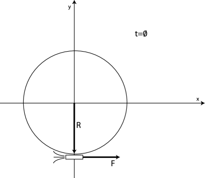
Figure 1: Position of spaceship/thruster combination at time $t=0$.

II.1 The solution to the problem

Three equations, one from the torque of the thruster, and the other two from the $x$ and $y$ components of the force of the thruster, define the motion. Let $\theta$ be the angle the thruster has rotated about its center of mass since time $t=0$. Initially, the ship will move in the $x$ direction and then upward into the first quadrant as it begins to rotate as shown in Fig. 2.

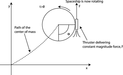
Figure 2: Qualitative sketch of the position of the spaceship/thruster combination shortly after $t=0$. The ship is rotating and translating.

From the torque on the system about the center of mass, the rotational analog of Newton’s second law ($\tau=I\ddot{\theta}$) requires

$$FR=c\,mR^{2}\ddot{\theta}$$ (1)

where the moment of inertia is $I=c\,mR^{2}$, where $c$ is a dimensionless constant that depends on the distribution of mass (e.g. $\frac{1}{2}$ for a disk, but in general any positive number), m is the mass of the ship, $R$ is the distance from the center of mass to the thruster, and $\ddot{\theta}$ is the second derivative of $\theta(t)$ with respect to time. Solving for the angle as a function of time we have

$$\theta(t)=\frac{Ft^{2}}{2c\,mR}$$ (2)

assuming $\theta(0)=\dot{\theta}(0)=0$. The case of $\dot{\theta}(0)\neq 0$ will be explored later in the paper.

Newton’s second law requires

$$F\cos(\theta)=m\ddot{x}$$ (3)

$$F\sin(\theta)=m\ddot{y}$$ (4)

where $x$ and $y$ are the coordinates of the center of mass. Substituting for $\theta$ and integrating these equations gives velocity components:

$$v_{x}(t)=\frac{F}{m}\int_{0}^{t}\cos(\frac{Ft^{\prime 2}}{2c\,mR})dt^{\prime}$$ (5)

$$v_{y}(t)=\frac{F}{m}\int_{0}^{t}\sin(\frac{Ft^{\prime 2}}{2c\,mR})dt^{\prime}$$ (6)

assuming $v_{x}(0)=v_{y}(0)=0$. These integrals are well studied and are called Fresnel integralsAbramowitz and Stegun (1972). Their evaluation is aided by a plot called the Cornu Spiral, which is shown in Fig. 3. Note the analysis required to this point was within the level of the typical elementary calculus-based physics course, though the integrals have led to special functions.

II.2 The motion of the center of mass and the Cornu Spiral

Examining the Fresnel integrals for the velocity components reveals much about the motion of the center of mass. In the limit $t\rightarrow\infty$, each component of velocity goes to $\sqrt{\pi cFR/4m}$. Therefore, the center of mass moves off at a $45$ degree angle with respect to the $x$-axis as time approaches infinity. The Cornu Spiral, most commonly associated with the problem of diffraction of a rectangular aperture Hecht (2002), represents these two integrals graphically. Fig. 3 is the Cornu Spiral as it is often displayed Abramowitz and Stegun (1972); Hecht (2002). A point on this spiral (when multiplied by the factor $\sqrt{\pi cFR/m}$) represents the $x$ and $y$ components of velocity at a point in time. A line drawn from the origin to a point on the spiral represents the instantaneous direction of the motion of the center of mass. Thus from this plot we see the center of mass is always in the first quadrant since $v_{x}$ and $v_{y}$ are always positive. And since $v_{x}$ is positive at all times then the plot of motion in the $y$ versus $x$ plane is single valued.

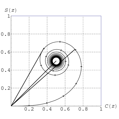
Figure 3: The Cornu Spiral as it is often shownHecht (2002); Abramowitz and Stegun (1972). The Fresnel sine integral, $S(z)=\int^{z}_{0}\sin(\frac{\pi}{2}t^{2})dt$, is plotted on the $y$-axis versus the Fresnel cosine integral, $C(z)=\int^{z}_{0}\cos(\frac{\pi}{2}t^{2})dt$, on the $x$-axis. The parameter $z$, proportional to time for our problem, runs along the spiral with a tick every $0.2$ stopping at 3.0. For the spaceship problem the axes are proportional to the $x$ and $y$ velocity components. The central portion of the spiral near $(0.5,0.5)$ is not plotted for clarity. The three straight lines on the plot represent the velocities with the steepest direction, the terminal speed, and the maximum speed, respectively in a clockwise fashion.

Fig. 3 also reveals a maximum speed (depicted by the longest straight line) which is approximately equal to $1.3422v_{\infty}$, where $v_{\infty}$ (straight line to center of spiral) represents the speed of the center of mass as time approaches infinity. The plot also shows a maximum angle with respect to the $x$-axis for the trajectory approximately equal to $60.466^{\circ}$, independent of any other parameters. Thus if the thruster is fired for an appropriate finite period of time, one could obtain a trajectory anywhere between zero and $60.466^{\circ}$ with respect to the x-axis, or a terminal velocity anywhere between zero and $1.3422v_{\infty}$.

II.3 The path of the center of mass

Integrating the velocity components, equations 5 and 6, gives the position of the center of mass:

$$x(t)=\frac{F}{m}\int_{0}^{t}\int_{0}^{t^{\prime\prime}}\cos(\frac{Ft^{\prime 2}}{2c\,mR})dt^{\prime}dt^{\prime\prime}$$ (7)

$$y(t)=\frac{F}{m}\int_{0}^{t}\int_{0}^{t^{\prime\prime}}\sin(\frac{Ft^{\prime 2}}{2c\,mR})dt^{\prime}dt^{\prime\prime}$$ (8)

where we have assumed $x(0)=y(0)=0$. These integrals can be evaluated numerically. Interestingly, using integration by parts the position can also be expressed analytically in terms of equations 5 and 6, the components of velocity. We find

$$x(t)=-cR\sin(\frac{Ft^{2}}{2c\,mR})+t\,v_{x}(t)$$ (9)

$$y(t)=cR[-1+\cos(\frac{Ft^{2}}{2c\,mR})]+t\,v_{y}(t).$$ (10)

Thus the path of motion can be studied analytically through the Fresnel special functions and its associated Cornu spiral.

A plot of the motion is shown in Fig. 4. The shape of the path is universal regardless of parameter values though distances are scaled by the factor $c\,R$. Note that the asymptotic trajectory as projected back towards the origin does not pass through the origin but has a non-zero $x$-intercept. Analytic analysis of the asymptotic ($t\rightarrow\infty$) forms of equations 9 and 10 show this intercept occurs $x=c\,R$. Curiously, while the thruster delivers equal $x$ and $y$ components of impulse (change in momentum) as time approaches infinity to the center of mass, there is an asymmetry in the displacement as shown by this intercept (due to $v_{x}$ being greater than $v_{y}$ initially). For actual spacecraft maneuvers we see a single thruster is not a very practical configuration.

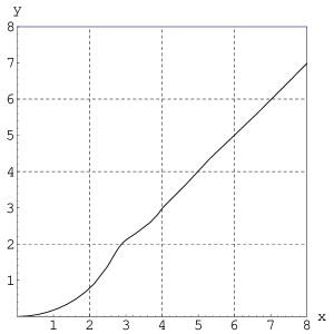
Figure 4: The path of the center of mass of the spaceship. For actual distances the axes should be multiplied by $c\,R$. The shape of this path is universal and doesn’t depend on other parameters save for the scaling factor $c\,R$.

III Physical Intuition

It has been our experience that the majority of students and faculty alike have difficulty intuiting the motion of the center of mass. Physical intuition is not a well defined term. An interesting recent book entitled Seeking Ultimates: An Intuitive Guide to Physics Landsberg (2000) states intuition is something for a student “to absorb in their bones.” The dictionary Suukhanov (1984) defines intuition as

1a) the act or faculty of knowing without the use of rational processes; immediate cognition b) knowledge acquired by use of this faculty. 2.) acute insight

We feel a definition of “physical intuition” requires more. A recent article by Singh Singh (2002) agrees that physical intuition is difficult to define but offers these words:

Cognitive theory suggests that those with good intuition can effectively pattern-match or map a given problem onto situations with which they have experience.

These words provide a suitable footing for the term because below we relate the problem at hand to a more common problem, which most physicists have had experience with during the course of their education. Perhaps “absorb in their bones” is on the mark if interpreted as absorbing a number of standard problems to provide a bank with which to pattern match.

III.1 Center of mass has a terminal velocity

The simplest idea is that as the object spins faster and faster the impulse to the center of mass over a single revolution must tend to zero. Therefore the change in linear momentum tends to zero and thus the notion of a terminal velocity for the center of mass is reasonable (though not guaranteed, the harmonic series tends to zero but it’s sum does not).

The first half of a revolution takes longer than the second and thus it must be the case that the impulse is always positive in the $y$ direction for any time and the motion is confined to the upper half plane. In addition, $y$ plotted as a function of time is monotonically increasing. One may be tempted to draw similar conclusions for the $x$ direction but here things are trickier, especially for whether a plot of $x$ versus time is monotonically increasing. To see this consider a slightly different problem.

III.2 An alternate spaceship problem

If the spaceship’s thruster had acted through its center of mass and had a rotation rate given by $\omega_{o}$, as pictured in Fig. 5, then we could say something about the $x$ component of velocity. During the first quarter of rotation the $x$ component of acceleration is positive and the $x$ component of velocity goes from $0$ to some maximum. During the second quarter of rotation the $x$ component of acceleration is negative and the symmetry of the applied force dictates that this acceleration will reduce the $x$ component of velocity to zero. During the last half of the rotation the $x$ component of velocity will be negative and the symmetry of the kinematics would return the $x$ component of the center of mass to $x=0$. Then, as far as the $x$ direction is concerned, the whole thing starts over again. The overall motion, assuming $\theta(t)=\omega_{o}t$, is a cycloid, reminiscent of the motion of a charged particle starting at rest in orthogonal uniform electric and magnetic fields.

The velocity components are

$$v_{x}(t)=\frac{F}{m\omega_{o}}\mathrm{sin}(\omega_{o}t)$$ (11)

$$v_{y}(t)=\frac{F}{m\omega_{o}}[1-\mathrm{cos}(\omega_{o}t)]$$ (12)

assuming $v_{x}=v_{y}=0$. And the positions would be given by

$$x(t)=\frac{F}{m\omega_{o}^{2}}[1-\mathrm{cos}(\omega_{o}t)]$$ (13)

$$y(t)=\frac{F}{m\omega_{o}^{2}}[\omega_{o}t-\mathrm{sin}(\omega_{o}t)].$$ (14)

The path is depicted in Fig. 6 and the shape of the path is also universal, though the axes are scaled by the factor $F/m\omega_{o}^{2}$. One possible mistake is to confuse constant rotation with uniform circular motion. But uniform circular motion is not a correct analogy since the force of the thruster is not, in general, perpendicular to the velocity of the center of mass.

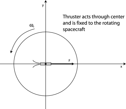
Figure 5: Sketch of the initial position for the alternate problem with the thruster acting through the center of mass but with the ship initially rotating at angular velocity $\omega_{o}$.

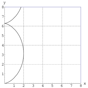
Figure 6: The cycloid motion of the center of mass for the alternate problem. The shape of the path is universal. The axes are in units of $F/m\omega_{o}^{2}$.

III.3 Spaceship is stuck in the first quadrant

Returning to the original problem, the rotation rate is not constant, but increases. As such we would expect the particle to never return to $x=0$ since the time spent in each rotation thrusting with a positive $x$ component will be longer than the time spent with a negative $x$ component. Thus the spaceship is doomed to remain in the first quadrant for all its travels contrary to a common misconception that the spaceship may move in some sort of spiral around the origin.

As mentioned earlier, we note the actual path of the center of mass as described by a function $y(x)$ is single-valued, meaning physically that the $x$ component of velocity (as well as the $y$ velocity component) is always positive. However, had there been an initial rotation, $\omega_{o}^{2}cmR/F=1$ for example, then there would have been a negative $x$ component of velocity during the first rotation and thus $y(x)$ would have been double valued for some $x$ values as shown in Fig. 7. The situation of a thruster with initial rotation is discussed in detail below.

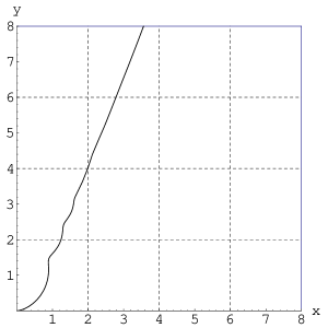
Figure 7: Path of motion of the center of mass for a situation with initial rotation. Again, as in Fig. 4 the shape of this path is fixed for a given value of $\omega_{o}^{2}cmR/F$, which in this case is $1$. The axes are in units of $c\,R$. Note the $x$ component of velocity is negative for a period during the first rotation (near $x=y=1$).

It is hoped the above discussion sheds some light on why the $45$-degree asymptotic path, the non-zero $x$-intercept, and the single-valued nature of $y(x)$ are difficult to intuit, even in hindsight. They depend on the value of integrals that are not intuitive (without the aid of the Cornu spiral or some other such device).

We did succeed in providing an “intuitive” explanation to explain that the path of motion is all in the first quadrant by comparing to an alternative known elementary problem. And, we intuited the notion of a terminal velocity and thus the asymptotic path for large times is a straight line.

In the interest of full disclosure, we add that our initial thoughts on the motion weren’t always right, and we wrote this section with the benefit of hindsight from solving the equations of motion.

IV Dimensional Analysis

Dimensional analysis has been discussed, for example, in association with models and data utilizing the simple pendulum as an example Price (2003), in a simple experiment involving the flow of sand Yersel (2000), and in the error analysis of a falling body Bohren (2004). This problem lends itself to dimensional analysis, the most interesting example being the terminal velocity. The characteristic mass is $m$, length is $R$, and time is $\sqrt{mR/F}$. A fourth parameter for the problem is actually dimensionless, the parameter $c$ from the form factor of the moment of inertia. Though dimensionless one can usually predict whether a quantity should increase or decrease as a function of $c$, though the power of the dependance on $c$ is unobtainable by such analysis.

Table 1 list a few quantities of possible interest, such as terminal velocity ($v_{\infty}$) and the $x$ intercept of the asymptotic path, along with the actual value and a dimensional estimate. Note all numerical prefactors of the estimates are within a factor of ten of the actual prefactor.

Table 1: Quantities of interest, dimensional estimates, and actual values for the problem with the thruster at the edge of the spaceship.

Quantity	Estimates	Actual
length	$R$	–
mass	$m$	–
time	$\sqrt{mR/F}$	–
$t_{1st~{}rotation}$	$\sqrt{mR/F}$	$\sqrt{4\pi c\,mR/F}$
$v_{\infty}$	$\sqrt{FR/m}$	$\sqrt{\pi cFR/2m}$
$x$ intercept of asymptotic path	$R$	$cR$
displacement($t_{1st~{}rotation}$)	$R$	$\sim 3.75cR$

IV.1 Dimensional analysis of the alternate problem

To physically understand the motion we introduced the alternate problem of a spaceship initially rotating with thrust acting through the center of mass. This effectively eliminates the radius, $R$, from the problem (since no torque is available the rotation rate will not change), but it introduced a new parameter, the initial rotation rate, $\omega_{o}$. For this problem the characteristic mass is $m$, length is $F/m\omega_{o}^{2}$, and time is $1/\omega_{o}$.

Table 2 is analogous to Table 1 for this alternate problem. Note again all numerical prefactors of the estimates are within a factor of ten of the actual prefactor.

Table 2: Quantities of interest, dimensional estimates, and actual values for the alternate problem with the thruster acting through the center of mass but with initial rotation, $\omega_{o}$.

Quantity	Estimates	Actual
length	$F/m\omega_{o}^{2}$	–
mass	$m$	–
time	$1/\omega_{o}$	–
$t_{1st~{}rotation}$	$1/\omega_{o}$	$2\pi/\omega_{o}$
$v_{drift}$	$F/m\omega_{o}$	$F/m\omega_{o}$
maximum $x$	$F/m\omega_{o}^{2}$	$2F/m\omega_{o}^{2}$
displacement($t_{1st~{}rotation}$)	$F/m\omega_{o}^{2}$	$2\pi F/m\omega_{o}^{2}$

IV.2 Original problem with initial rotation

If the original problem had been initially rotating then there would have been two length scales, two time scales, and even two mass scales. The second mass scale would be given by $F/R\omega_{o}^{2}$. With two sets of characteristic scales, dimensional analysis is of less value because there are an infinite number of ways to construct quantities of interest. For example, let $l_{1},m_{1},t_{1}$ be a characteristic length, mass and time respectively, and let $l_{2},m_{2},t_{2}$ be a second set. Suppose we’re curious about a velocity. Obvious possibilities are $l_{1}/t_{1}$ and $l_{2}/t_{2}$. But

$$\frac{l_{1}}{t_{2}},\hskip 7.22743pt\sqrt{\frac{l_{1}l_{2}}{t_{1}t_{2}}},\hskip 7.22743pt\frac{l_{1}m_{2}}{t_{1}m_{1}},\hskip 7.22743pt\mathrm{or}\hskip 7.22743pt\sqrt{\frac{m_{2}}{m_{1}}}\left({\frac{l_{1}}{t_{1}}}\right)$$ (15)

are examples of other possibilities.

Consider the initial problem but now allow an initial rotation rate as well. The velocity components would be given by the integrals:

$$v_{x}(t)=\frac{F}{m}\int_{0}^{t}\cos({\frac{Ft^{\prime 2}}{2c\,mR}}+\omega_{o}t^{\prime})dt^{\prime}$$ (16)

$$v_{y}(t)=\frac{F}{m}\int_{0}^{t}\sin({\frac{Ft^{\prime 2}}{2c\,mR}}+\omega_{o}t^{\prime})dt^{\prime}.$$ (17)

Our intuition says the terminal velocity should decrease as $\omega_{o}$ increases (for positive $\omega_{o}$, i.e. in the direction of the applied torque). Dimensional analysis for a velocity reveals ambiguities such as:

$$\frac{F^{2}}{\omega_{o}^{3}cRm^{2}},\hskip 7.22743pt\frac{F^{3/2}}{\omega_{o}^{2}c^{1/2}R^{1/2}m^{3/2}},\hskip 7.22743pt\frac{F}{\omega_{o}m}.$$ (18)

The new velocity integrals can still be interpreted with the aid of the Cornu spiral. By completing the square of the arguments of the trigonometric functions, an initial rotation can be shown to be a shift of $\sqrt{\omega^{2}_{o}c\,mR/\pi F}$ along the spiral and a rotation of axis by an angle of $\omega^{2}_{o}c\,mR/2F$ as shown in Fig. 8, where the shifted axes are placed for an initial rotation satisfying $\omega_{o}^{2}cmR/F=1$.

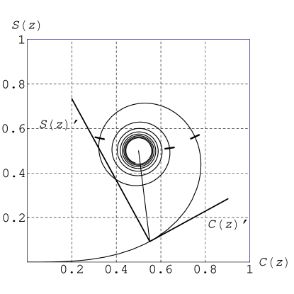
Figure 8: The Cornu spiral is shown with a new axis placed along the spiral to account for an initial rotation satisfying $\omega_{o}^{2}cmR/F=1$. Note the trajectory angle of the line which is proportional to $v_{\infty}$ (line from the new origin to the point $\frac{1}{2},\frac{1}{2}$) is parallel to the asymptotic trajectory in Fig. 7 above. The ticks placed along the spiral represent other origins corresponding to $\omega_{o}^{2}cmR/F=4,9$ and $16$. As in Fig. 3 actual velocities are obtained by multiplying the axes by the factor $\sqrt{\pi cFR/m}$.

With the aid of this shifted axis, we see the terminal velocity should indeed get smaller and also the angle of the trajectory should increase. Also, both $v_{x}$ and $v_{y}$ should approach zero as $\omega_{o}$ approaches infinity. However, since the trajectory tends to $90$ degrees from the $x$-axis as $\omega_{o}\rightarrow\infty$ we note $v_{x}$ and $v_{y}$ cannot tend to zero with the same dependence on $\omega_{o}$.

In fact, it can be shown that as $\omega_{o}\rightarrow\infty$

$$v_{x}(t=\infty)\sim\frac{F^{2}}{\omega_{o}^{3}cRm^{2}}-\frac{3F^{4}}{\omega_{o}^{7}c^{3}R^{3}m^{4}}+{\cal O}\left(\frac{1}{\omega^{11}_{o}}\right)$$ (19)

and

$$v_{y}(t=\infty)\sim\frac{F}{\omega_{o}m}-\frac{3F^{3}}{\omega_{o}^{5}c^{2}R^{2}m^{3}}+{\cal O}\left(\frac{1}{\omega^{9}_{o}}\right).$$ (20)

Each term in the expansions are further examples of the ambiguity in constructing velocities with two characteristic scales. The asymptotic trajectory (angle from the $x$-axis) approaches $90$ degrees, since $\tan(\theta)=(v_{y}/v_{x})\sim\omega_{o}^{2}cRm/F$ as $\omega_{o}\rightarrow\infty$.

V Path of motion with a negative initial rotation

Since we have just generalized the original problem to include a non-zero initial rotation aligned with the applied torque, it is interesting to consider a negative initial rotation, i.e. initially spinning opposite the direction of the applied torque. Fig. 9 displays the path of the center of mass for the situation $\omega_{o}^{2}cmR/F=25$ and with $\omega_{o}$ being negative (i.e. opposite the direction of the torque). Notice that the displacement vector, for this case, sweeps a polar angle somewhere between 270 and 360 degrees. This raises questions: What is the maximum this angle could be? Could the spaceship spiral around the origin, with an appropriate initial rotation, as some incorrectly suggest for the original problem with no initial rotation? Our explorations reveal that with an appropriate choice of a negative $\omega_{o}$ the asymptotic path can be any compass heading in the full 360 degree range of possibilities.

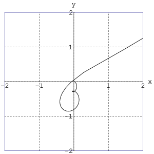
Figure 9: The path of the center of mass for a situation with initial rotation opposite the applied torque of the thruster, assuming $\omega_{o}^{2}cmR/F=25$. Axes are in units of the factor $cR$.

Fig. 10 shows four such possibilities associated with four different initial rotation rates.

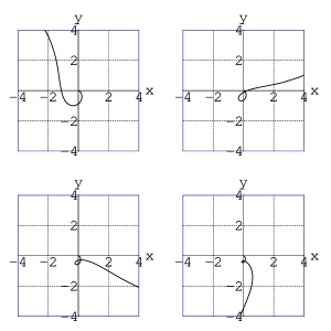
Figure 10: The path of the center of mass for a situation with initial rotation opposite the applied torque of the thruster, with $\omega_{o}=-3.2,-3.6,-3.8$ and $-4.2$ respectively in units of $\sqrt{F/cmR}$ (left to right then top to bottom). Axes are in units of the factor $cR$.

V.1 Can the center of mass circle the origin? No

As before, using integration by parts the components of position can be expressed in terms of the velocity components. We find:

$$x(t)=-cR\sin(\frac{Ft^{2}}{2cmR}+\omega_{o}t)+(t+\frac{\omega_{o}cmR}{F})v_{x}(t)$$ (21)

$$y(t)=cR[\cos(\frac{Ft^{2}}{2cmR}+\omega_{o}t)-1]+(t+\frac{\omega_{o}cmR}{F})v_{y}(t)$$ (22)

where $v_{x}(t)$ and $v_{y}(t)$ are those given by equations 16 and 17 respectively. For the spaceship to circle the origin a necessary, but not sufficient, condition is that $v_{y}=0$ while $y>0$. Examining equation 22, we see that if $v_{y}=0$ then

$$y\arrowvert_{v_{y}=0}=cR[\cos(\frac{Ft^{2}}{2cmR}+\omega_{o}t)-1]$$ (23)

must be positive if we are to meet this condition. But this cannot ever be true since the most the cosine term could be is $1$. Therefore once $y>0$ the spaceship will remain in the upper half plane. Note the above proof does not require any properties of the Fresnel functions, just integration by parts.

V.2 What is the displacement vector’s maximum polar angle?

Numerically, we have determined the maximum angle the displacement vector can sweep while going around the origin is approximately $319.52^{\circ}$ which occurs when the initial rotation rate is approximately $\omega_{o}\approx-3.54$ in units of $\sqrt{F/cmR}$. At approximately $\omega_{o}=-5.01$, which is near that depicted in Fig. 9 the path again approaches intersection with the origin with a corresponding maximum polar angle for the displacement vector of approximately $318.27^{\circ}$. There are infinitely many more of these pairs; the list begins like this

$$\matrix{\omega_{o,1}\approx-3.54491&\hskip 21.68121pt\theta_{1,t=\infty}\approx 319.522^{\circ}\cr\omega_{o,2}\approx-5.01326&\hskip 21.68121pt\theta_{2,t=\infty}\approx 318.272^{\circ}\cr\omega_{o,3}\approx-6.13996&\hskip 21.68121pt\theta_{3,t=\infty}\approx 317.682^{\circ}\cr\omega_{o,4}\approx-7.08982&\hskip 21.68121pt\theta_{4,t=\infty}\approx 317.327^{\circ}\cr\vdots\hskip 14.45377pt&\hskip 43.36243pt\vdots\hskip 21.68121pt.}$$ (24)

The maximum polar angle appears to continue to decrease. Thus $319.52^{\circ}$ appears to be the approximate maximum regarding encircling the origin. A plot of the polar angle swept by the displacement vector ($\theta_{displacement}$) from $t=0$ to $t=\infty$ is shown versus the initial rotation ($\omega_{o}$) in Fig. 11 in units of $\sqrt{F/cmR}$.

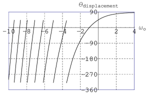
Figure 11: The polar angle swept by the displacement vector (in degrees) from $t=0$ to $t=\infty$ as a function of the initial rotation rate $\omega_{o}$ in units of $\sqrt{F/cmR}$. The discontinuities correspond to paths that intersect the origin. Thus, qualitatively, at the discontinuity the path went from one like that in Fig. 9 where it was going around the origin to one like that in the top right of Fig. 10 where it cut back below the origin. The maximum angles referred to in the text are defined as negative angles on this plot.

VI Conclusion

As one object (see appendix), one force problems go, this one may rival the simple harmonic oscillator for its richness. The problem has utility in introducing a student to special functions and handbooks such as Abromowitz and Stegun Abramowitz and Stegun (1972). It also provides a mechanical model for thinking about Fresnel integrals. It could be used in a numerical methods course where comparison between analytic (and analytic asymptotic) expressions versus numerical techniques could be performed. The dimensional analysis applied to this problem is useful for many other problems. For example, projectile motion possesses a universal path shape, a parabola, characterized by the dimensionless parameter the launch angle with the length scale set by $v_{o}^{2}/g$ where $v_{o}$ is the initial velocity and $g$ the acceleration due to gravity. When presenting a new problem to a student, a good question to ask is to try to sort out how many sets of scales does the problem encompass and what can dimensional arguments say about the answers to any questions posed. Finally, the problem is a challenging test of physical intuition and it can be of interest to the teacher and student alike to think about just what is meant by such a term as “physical intuition” and how would one go about improving it.

Appendix A The other object(s) - momentum conservation

The title stated there is only one body in this problem and indeed the spaceship with its attached thruster has been our focus. But momentum conservation suggests this cannot be the only thing in our universe. The thruster must be emitting something (perhaps a photon) that carries momentum (and also energy and angular momentum). The momentum is carried away in all directions since the spaceship rotates. The magnitude of the instantaneous impulse imparted by the thruster, is $Fdt$. The impulse per angular bin from $\theta$ to $\theta+d\theta$ as a function of $\theta$ using Eq. 2 is then:

$$\frac{Fdt}{d\theta}=\sqrt{\frac{Fc\,mR}{2\theta}}.$$ (25)

A plot of this impulse density over the first cycle is shown in Fig. 12.

Integrating the $x$-component, for example, over one revolution (from $0$ to $2\pi$) should be equivalent to evaluating Eq. 5 multiplied by $m$ from $t=0$ to $\sqrt{4\pi c\,mR/F}$, i.e.

$$F\int_{0}^{\sqrt{\frac{4\pi c\,mR}{F}}}\cos(\frac{Ft^{2}}{2c\,mR})dt=\int_{0}^{2\pi}\sqrt{\frac{FcmR}{2\theta}}\cos(\theta)d\theta$$ (26)

With the substitution $\theta=Ft^{2}/2c\,mr$ this is shown to be true. In fact an alternative representation of the Fresnel cosine integral isAbramowitz and Stegun (1972):

$$\int_{0}^{a}\cos(t^{2})dt=\frac{1}{2}\int_{0}^{a^{2}}\frac{\cos(x)}{\sqrt{x}}dx.$$ (27)

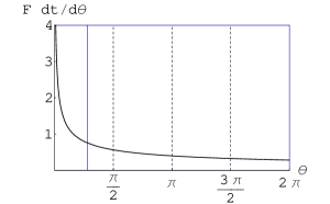
Figure 12: The distribution of $Fdt/d\theta$ during the first rotation as a function of the rotation angle. The average over the first cycle occurs at $\sim 50.77^{\circ}$ ($\sim 0.886$ radians and denoted by a solid grid line), which is near that of the asymptotic path of $45$ degrees.

References

- Abramowitz and Stegun (1972) M. Abramowitz and I. A. Stegun, Handbook of Mathematical Functions with Formulas, Graphs, and Mathematical Tables (Dover Publications, New York, 1972).
- Hecht (2002) E. Hecht, Optics (Addison-Wesley, San Francisco, 2002), 4th ed.
- Landsberg (2000) P. T. Landsberg, Seeking Ultimates An Intuitive Guide to Physics (Institute of Physics Publishing, Philadelphia, 2000).
- Suukhanov (1984) A. H. Suukhanov, ed., Webster’s II New Riverside University Dictionary (Houghton Mifflin Company, Boston, 1984).
- Singh (2002) C. Singh, Am. J. Phys. 70, 1103 (2002).
- Price (2003) J. F. Price, Am. J. Phys. 71, 437 (2003).
- Yersel (2000) M. Yersel, The Physics Teacher 38, 290 (2000).
- Bohren (2004) C. F. Bohren, Am. J. Phys. 72, 534 (2004).