Complex States of Simple Molecular Systems

Abstract

A review is given of phase properties in molecular wave functions, composed of a number of (and, at least, two) electronic states that become degenerate at some nearby values of the nuclear configuration. Apart from discussing phases and interference in classical (non-quantal) systems, including light-waves, the review looks at the constructability of complex wave functions from observable quantities (”the phase problem”), at the controversy regarding quantum mechanical phase-operators, at the modes of observability of phase and at the role of phases in some non-demolition measurements. Advances in experimental and (especially) theoretical aspects of Aharonov-Bohm and topological (Berry) phases are described, including those involving two-electron and relativistic systems. Several works in the phase control and revivals of molecular wave-packets are cited as developments and applications of complex-function theory. Further topics that this review touches on are: coherent states, semiclassical approximations and the Maslov index. The interrelation between time and the complex state is noted in the contexts of time delays in scattering, of time-reversal invariance and of the existence of a molecular time-arrow.

When the stationary Born-Oppenheimer description for nearly degenerate state is regarded as ”embedded” in a broader dynamic formulation, namely through solution of the time dependent Schrödinger equation, the wave function becomes necessarily complex. The analytic behavior of this function in the complex time-plane can be exploited to gain information about the connection between phases and moduli of the component-amplitudes. One form of this connection are a pair of reciprocal (Kramers-Kronig type) relations in the complex time-domain. These show that certain phase changes in a component amplitude (such as, e.g., lead to a non-zero Berry-phase) require changes in the amplitude-moduli, too, and imply degeneracies of the electronic state.

The subject of conical degeneracy, or intersection, of adjacent potential surface is extended to nonlinear nuclear-electronic coupling, which can then result in multiple conical degeneracies on a nuclear coordinate plane. We treat cases of double and fourfold intersections, the latter under trigonal symmetry, and employ an analytic-graphical phase tracing method to obtain the resulting Berry phases as the system circles around some or all of the degeneracy points. These phases can take up values that are all integral multiples of $\pi$, with integers that vary with the physical situation (or with the model postulated for it).

A further type of invariance, with respect to gauge transformation, is also tied to the complex form of the wave function. For a many-component state this leads to a consideration of tensorial (Yang-Mills type) fields $F$ for molecular systems. It is shown that it is the truncation of the Born-Oppenheimer electron-nuclear superposition that generates the molecular Yang-Mills fields.

The equations of motion for the nuclear degrees of freedom are derived from a Lagrangean density $\cal L$, representing a non-Abelian situation. In $\cal L$ the non-adiabatic coupling terms (NACTs), that express the electronic background on the nuclear states, enter as vector potentials (or gauge fields). We demonstrate a deep lying interrelation between two apparently distinct theoretical developments: that which led to the discovery of the Yang-Mills fields from considerations of local gauge-invariance, and the use of an adiabatic-diabatic transformation matrix for the molecular case due to Baer. A generalized form of the NACTs is found, such that it makes the field $F$ vanish for a complete electronic set.

Lastly, the use of phases and moduli as variables was found to be very convenient to obtain variationally the equation of continuity and the Hamilton-Jacobi equations from the Lagrangian of an electron following either the Schrödinger or the Dirac equation. In the latter case, to a good approximation (in the nearly non-relativistic limit) the phases in the different spinor components are not scrambled together and their Berry phases are unaffected.

PACS numbers: 03.65.Bz, 03.65.Ca, 03.65.Ge, 31.15.-p, 31.30.-i, 31.30.Gs, 31.70.-f

keywords: phases, Born-Oppenheimer states, nonadiabatic coupling

Chapter 1 Complex States of Simple Molecular Systems

1.1 Introduction and Preview of the Chapter

In quantum theory physical systems move in vector spaces that are, unlike those in classical physics, essentially complex. This difference has had considerable impact on the status, interpretation and mathematics of the theory. These aspects will be discussed in this Chapter within the general context of simple molecular systems, while concentrating, at the same time, on instances in which the electronic states of the molecule are exactly or nearly degenerate. It is hoped that as the Chapter progresses, the reader will obtain a clearer view of the relevance of the complex description of the state to the presence of a degeneracy.

The difficulties that arose from the complex nature of the wave function during the development of quantum theory are recorded by historians of science ([1] - [3]). For some time during the early stages of the new quantum theory the existence of a complex state defied acceptance ([1], p.266). Thus, both de Broglie and Schrödinger believed that material waves (or ”matter” or ”de Broglie” waves, as they were also called) are real (i.e., not complex) quantities, just as electromagnetic waves are [3]. The decisive step for the acceptance of the complex wave came with the probabilistic interpretation of the theory, also known as Born’s probability postulate. This placed the modulus of the wave function in the position of a (and, possibly, unique) connection between theory and experience. This development took place in the year 1926 and it is remarkable that already in the same year Dirac embraced the modulus based interpretation wholeheartedly [4]. [Oddly, it was Schrödinger who appears to have, in 1927, demurred at accepting the probabilistic interpretation ([2], p. 561, footnote 350)]. Thus, the complex wave function was at last legitimated, but the modulus was and has remained for a considerable time the focal point of the formalism.

A somewhat different viewpoint motivates this article, which stresses the added meaning that the complex nature of the wave function lends to our understanding. Though it is only recently that this aspect has come to the forefront, the essential point was affirmed already in 1972 by Wigner [5] in his famous essay on the role of mathematics in physics. We quote from this here at some length:

”The enormous usefulness of mathematics in the natural sciences is something bordering on the mysterious and there is no rational explanation for … this uncanny usefulness of mathematical concepts…

The complex numbers provide a particularly striking example of the foregoing. Certainly, nothing in our experience suggests the introducing of these quantities… Let us not forget that the Hilbert space of quantum mechanics is the complex Hilbert space with a Hermitian scalar product. Surely to the unpreoccupied mind, complex numbers … cannot be suggested by physical observations. Furthermore, the use of complex numbers is not a calculational trick of applied mathematics, but comes close to being a necessity in the formulation of the laws of quantum mechanics. Finally, it now [1972] begins to appear that not only complex numbers but analytic functions are destined to play a decisive role in the formulation of quantum theory. I am referring to the rapidly developing theory of dispersion relations. It is difficult to avoid the impression that a miracle confronts us here [i.e., in the agreement between the properties of the hypernumber $\sqrt{(}-1)$ and those of the natural world].”

A shorter and more recent formulation is: ”The concept of analyticity turns out to be astonishingly applicable”([6], p.37)

What is addressed by these sources is the ontology of quantal description. Wave functions (and other related quantities, like Green functions or density matrices), far from being mere compendia or short-hand listings of observational data, obtained in the domain of real numbers, possess an actuality of their own. From a knowledge of the wave functions for real values of the variables and by relying on their analytical behavior for complex values, new properties come to the open, in a way that one can perhaps view, echoing the quotations above, as ”miraculous”.

A term that is nearly synonymous with complex numbers or functions is their ”phase”. The rising preoccupation with the wave function phase in the last few decades is beyond doubt, to the extent that the importance of phases has of late become comparable to that of the moduli. (We use Dirac’s terminology [7], that writes a wave function by a set of coefficients, the “amplitudes”, each expressible in terms of its absolute value, its “modulus”, and its ”phase”). There is a related growth of literature on interference effects, associated with Aharonov-Bohm and Berry phases ([8] - [14]). In parallel, one has witnessed in recent years a trend to construct selectively and to manipulate wave functions.The necessary techniques to achieve these are also anchored in the phases of the wave function components. This trend is manifest in such diverse areas as coherent or squeezed states [15, 16], electron transport in mesoscopic systems [17], sculpting of Rydberg-atom wave-packets [18, 19], repeated and non-demolition quantum measurements [20], wave-packet collapse [21] and quantum computations [22, 23]. Experimentally, the determination of phases frequently utilize measurement of Ramsey fringes [24] or similar methods [25].

The status of the phase in quantum mechanics has been the subject of debate. Insomuch as classical mechanics has successfully formulated and solved problems using action-angle variables [26], one would have expected to see in the phase of the wave-function a fully ”observable” quantity, equivalent to and and having a status similar to the modulus, or to the equivalent concept of the ”number variable”. This is not the case and, in fact, no exact, well behaved Hermitean phase operator conjugate to the number is known to exist. [An article by Nieto [27] describes the early history of the phase operator question, and gives a feeling of the problematics of the field. An alternative discussion, primarily related to phases in the electromagnetic field, is available in [28]]. In section 2 a brief review is provided of the various ways that phase is linked to molecular properties.

Section 3 presents results that the analytic properties of the wave function as a function of time $t$ imply and summarizes previous publications of the authors and of their collaborators ([29] -[38]). While the earlier quote from Wigner has prepared us to expect from the analytic behavior of the wave function some general insight, the equations in this section yield the specific result that, due to the analytic properties of the logarithm of wave function amplitudes, certain forms of phase changes lead immediately to the logical necessity of enlarging the electronic set or, in other words, to the presence of an (otherwise) unsuspected state.

In the same section we also see that the source of the appropriate analytic behavior of the wave function is outside its defining equation, (the Schrödinger equation), and is in general the consequence of either some very basic consideration or of the way that experiments are conducted. The analytic behavior in question can be in the frequency or in the time domain and leads in either case to a Kramers-Kronig type of reciprocal relations. We propose that behind these relations there may be an ”equation of restriction”, but while in the former case (where the variable is the frequency) the equation of restriction expresses causality (”no effect before cause”), for the latter case (when the variable is the time), the restriction is in several instances the basic requirement of lower boundedness of energies in (no-relativistic) spectra ([39, 40]). In a previous work it has been shown that analyticity plays further roles in these reciprocal relations, in that it ensures that time-causality is not violated in the conjugate relations and that (ordinary) gauge invariance is observed [40].

As already remarked, the results in section 3 are based on dispersions relations in the complex time domain. A complex time is not a new concept. It features in wave optics [28] for ”complex analytic signals” (which is an electromagnetic field with only positive frequencies) and in non-demolition measurements performed on photons [41]. For transitions between adiabatic states (which is also discussed in this review), it was previously introduced in several works ([42] - [45]).

Interestingly, the need for a multiple electronic set, which we connect with the reciprocal relations, was also a keynote of a recent review ([46] and previous publications cited there and in [47]). Though the considerations relevant to this effect are not linked to complex nature of the states (but rather to the stability of the adiabatic states in the real domain), we have included in section 3 a mention of, and some elaboration on, this topic.

In further detail, section 3 stakes out the following claims: For time dependent wave functions rigorous conjugate relations are derived between analytic decompositions (in the complex t-plane) of phases and of $\log\ moduli$. This entails a reciprocity, taking the form of Kramers-Kronig integral relations (but in the time domain), holding between observable phases and moduli in several physically important cases. These cases include the nearly adiabatic (slowly varying) case, a class of cyclic wave-functions, wave packets and non-cyclic states in an ”expanding potential”. The results define a unique phase through its analyticity properties and exhibit the interdependence of geometric-phases and related decay probabilities. It turns out that the reciprocity property obtained in this section holds for several textbook quantum mechanical applications (like the minimum width wave packet).

The multiple nature of electronic set becomes especially important when the potential energy surfaces of two (or more) electronic states come close, namely, near a ”conical intersection” (ci). This is also the point in the space of nuclear configurations at which the phase of wave function components becomes anomalous. The basics of this situation have been extensively studied and have been reviewed in various sources ([49]- [51]). Recent works ([52] - [58]) have focused attention on a new contingency: when there may be several ci’s between two adiabatic surfaces, their combined presence needs to be taken into account for calculations of the non-adiabatic corrections of the states and can have tangible consequences in chemical reactions. Section 4 presents an analytic modeling of the multiple ci model, based on the superlinear terms in the coupling between electronic and nuclear motion. The section describes in detail a tracing method that keeps track of the phases, even when these possess singular behavior (namely, at points where the moduli vanish or become singular). The continuous tracing method is applicable to real states (including stationary ones). In these the phases are either zero or $\pi$. [At this point, it might be objected that in so far that numerous properties of molecular systems (e.g., those relating to questions of stability and, in general, to static situations and not involving a magnetic field) are well described in terms of real wave functions, the complex form of the wave function need, after all, not be regarded as a fundamental property. However, it will be shown in Section 4 that wave functions that are real but are subject to a sign change, can be best treated as limiting cases in complex variable theory. In fact, the ”phase tracing” method is logically connected to the time dependent wave-functions (and represents a case of mathematical ”embedding”)].

A specific result in Section 4 is the construction of highly non-linear vibronic couplings near a ci. The construction shows, inter alia, that the connection between the Berry (or ”topological”, or ”geometrical”) phase, acquired during cycling in a parameter space, and the number of ci’s circled depends on the details of the case that is studied and can vary from one situation to another. Though the subject of Berry phase is reviewed in a companion chapter in this volume [59], we note here some recent extensions in the subject ([60] - [62]). In these works, the phase changes were calculated for two-electron wave functions, such that are subject to inter-electronic forces . An added complication was also considered, for the case in which the two electrons are acted upon by different fields. This can occur when the two electrons are placed in different environments, as in asymmetric dimers. By and large, intuitively understandable results are found for the combined phase factor but, under conditions of accidental degeneracies, surprising jumps ( named ”switching”) are noted. Some applications to quantum computations seem to be possible [62].

The theory of Born-Oppenheimer (abbreviated to BO) [63, 64] has been hailed (in an authoritative but unfortunately unidentified source) as one of the greatest advances in theoretical physics. Its power is in disentangling the problem of two kinds of interacting particles into two separate problems, ordered according to some property of the two kinds. In its most frequently encountered form, it is the nuclei and electrons that interact (in a molecule or in a solid) and the ordering of the treatment is based on the large difference between their masses. However, other particle pairs can be similarly handled, like hadronic mesons and baryons, except that a relativistic or field theoretical version of the Born-Oppenheimer theory is not known. The price that is paid for the strength of the method is that the remaining coupling between the two kinds of particles is dynamic. This coupling is expressed by the so called Non-Adiabatic Coupling Terms (abbreviated as NACTs), which involve derivatives of (the electronic) states rather than the states themselves. ”Correction terms” of this form are difficult to handle by conventional perturbation theory. For atomic collisions the method of ” Perturbed Stationary States” was designed to overcome this difficulty [65, 66], but this is accurate only under restrictive conditions. On the other hand, the circumstance that this coupling is independent of the potential, indicates that a general procedure can be used to take care of the NACTs [68]. Such general procedure was developed by Yang and Mills in 1954 [68] and has led to far reaching consequences in the theory of weak and strong interactions between elementary particles.

The interesting history of the Yang-Mills field belongs essentially to particle physics ([69] - [72]). The reason for mentioning it here in a chemical physics setting, is to note that an apparently entirely different procedure was proposed for the equivalent problem arising in the molecular context, namely, for the elimination of the derivative terms (the NACTs) from the nuclear part of the BO Schrödinger equation through an Adiabatic-Diabatic Transformation (ADT) matrix [67, 48]. It turns out that the quantity known as the tensorial field (or covariant, or Yang-Mills, or YM field, with some further names also in use) enters also into the ADT description, though from a completely different viewpoint, namely through ensuring the validity of the ADT matrix method by satisfaction of what is known as the ”curl cndition”. Formally, when the ”curl condition” holds, the (classical) Yang-Mills field is zero and this is also the requirement for the strict validity of the ADT method. [A review of the ADT and alternative methods is available in, e.g., [49, 50], the latter of which discusses also the Yang-Mills field in the context of the BO treatment.] However, it has recently been shown by a formal proof, that an approximate construction of the ADT matrix (using only a finite, and in practice small, number of BO, adiabatic states) is possible even though the ”curl condition” may be formally invalid [36]. An example for such an approximate construction in a systematic way was provided in a model that uses Mathieu functions for the BO electronic states [73].

As has been noted some time ago, the non-adiabatic coupling terms (NACTs, mentioned above) can be incorporated in the nuclear part of the Schrödinger equation as a vector potential [74, 75]. The question of a possible magnetic field, associated with this vector potential has also been considered ([76] - [83]). For an electron occupying an admixture of two or more states (a case that is commonly designated as non-commutative, ”non-Abelian”), the fields of physical interest are not only the magnetic field, being the curl of the ”vector potential”, but also tensorial (Yang-Mills) fields. The latter is the sum of the curl field and of a vector-product term of the NACTs. Physically these field represent the reaction of the electron on the nuclear motion via the NACTs.

In a situation characteristic of molecular systems, a conical intersection ci arises from the degeneracy point of adiabatic potential energy surfaces in a plane of nuclear displacement coordinates. There are also a number of orthogonal directions, representing a so-called ”seam” direction. In this setting, it emerges that both kinds of fields are aligned with the seam direction of the ci and are zero everywhere outside the seam, but they differ as regards the flux that they produce. Already in a two-state situation, the fields are representation dependent and the values of the fluxes depend on the states the electron occupies. (This evidently differs from conventional electro-magnetism, in which the magnetic field and the flux are unchanged under a gauge transformation.)

Another subject in which there are implications of phase is the time evolution of atomic or molecular wave-packets. In some recently studied cases these might be a superposition of a good ten or so energy eigen-states. Thanks to the availability of short, femtosecond laser pulses both the control of reactions by coherent light ([16], [84]- [94]) and the probing of phases in a wave packet are now experimental possibilities ([19], [95] - [97]). With short duration excitations the initial form of the wave packet is a real ”doorway state” ([98]- [100]) and this develops phases for each of its component amplitudes as the wave-packet evolves. It has recently been shown that the phases of these components are signposts of a time arrow ([101]-[102]) and of the irreversibility; both of these are inherent in the quantum mechanical process of preparation and evolution [34]. It was further shown in [34] (for systems that are invariant under time-reversal, e.g. in the absence of a magnetic field) that the preparation of an initially complex wave-packet requires finite times for its construction (and cannot be achieved instantaneously).

The quantum phase factor is the exponential of an imaginary quantity ($i$ times the phase) which multiplies into a wave function. Historically, a natural extension of this was proposed in the form of a gauge transformation, which both multiplies into and admixes different components of a multi-component wave function [103]. The resulting ”gauge theories” have become an essential tool of quantum field theories and provide (as already noted in the discussion of the YM field, above) the modern rationale of basic forces between elementary particles ([69] -[72]). It has already been noted in an earlier paragraph, that gauge theories have also made notable impact on molecular properties, especially under conditions that the electronic state basis in the molecule consists of more than one component. This situation also characterizes the conical intersections between potential surfaces, as already mentioned. In section 5 we show how an important theorem, originally due to Baer [48], and subsequently used in several equivalent forms, gives some new insight to the nature and source of these YM fields in a molecular (and perhaps also in a particle-field) context. What the above theorem shows is that it is the truncation of the BO set that leads to the YM fields, whereas for a complete BO set the field is inoperative for molecular vector potentials.

Section 6 shows the power of the modulus-phase formalism and is included in this review partly for methodological purposes. In this formalism the equations of continuity and the Hamilton-Jacobi equations can be naturally derived in both the non-relativistic and the relativistic (Dirac) theories of the electron. It is shown that in the four-component (spinor) theory of electrons, the two extra components in the spinor wave-function will have only a minor effect on the topological phase, provided certain conditions are met (nearly non-relativistic velocities and external fields that are not excessively large).

So as to make the individual sections self-contained, we have found it advisable to give some definitions and statements more than once.

1.2 Aspects of Phase in Molecules

This section attempts a brief review of several areas of research on the significance of phases, mainly for quantum phenomena in molecular systems. Evidently, due to limitation of space, one cannot do justice to the breadth of the subject and numerous important works will go unmentioned. It is hoped that the several cited papers (some of which have been chosen from quite recent publications) will lead the reader to other, related and earlier, publications. It is essential to state at the outset that the overall phase of the wave-function is arbitrary and only the relative phases of its components are observable in any meaningful sense. Throughout, we concentrate on the relative phases of the components. (In a coordinate representation of the state function, the ”phases of the components” are none other than the coordinate-dependent parts of the phase, so it is also true that this part is susceptible to measurement. Similar statements can be made in momentum, energy, etc. representations.)

A further preliminary statement to this section would be that, somewhat analogously to classical physics or mechanics where positions and momenta (or velocities) are the two conjugate variables that determine the motion, moduli and phases play similar roles. But the analogy is not perfect. Indeed, early on it was questioned, apparently first by Pauli [104], whether a wave function can be constructed from the knowledge of a set of moduli alone. It was then argued by Lamb [105] that from a set of values of wave function moduli and of their rates of change, the wave function, including its phase, is uniquely found. Counter-examples were then given [106, 107] and it now appears that the knowledge of the moduli and some information on the analytic properties of the wave function are both required for the construction of a state. (The following section contains a formal treatment, based partly on [30] - [32] and [108]- [109].) In a recent research effort, states with definite phases were generated for either stationary or traveling type of fields [110].

Recalling for a start phases in classical waves, these have already been the subject of consideration by Lord Rayleigh [111], who noted that through interference between the probed and a probing wave the magnitude and phase of acoustic waves can be separately determined, e.g., by finding surfaces of minimum and of zero magnitudes. A recent review on classical waves is given by Klyshko [112]. The work of Pancharatnam on polarized light beams ([113, 114]) is regarded as the precursor of later studies of topological phases in quantum systems [9]. This work contained a formal expression for the relative phase between beams in different elliptic polarizations of light, as well as a construction (employing the so-named ”Poincare sphere”) that related the phase difference to a geometrical, area concept. (For experimental realizations with polarized light beams we quote [115, 116]; the issue of any arbitrariness in experimentally pinning down the topological part of the phase was raised in [118].) Regarding the interesting question of any common ground between classical and quantal phases, the relation between the adiabatic (Hannay’s) angle in mechanics and the phase in wave functions was the subject of [117]. The difference in two-particle interference patterns of electromagnetic and matter waves was noted, rather more recently, in [119]. The two phases, belonging to light and to the particle wave-function, are expected to enter on an equal footing when the material system is in strong interaction with an electromagnetic field (as in the Jaynes-Cummings model). An example of this case was provided in a study of a two level atom, which was placed in a cavity containing an electromagnetic field. Using one or two photon excitations, it was found possible to obtain from the Pancharatnam phase an indication of the statistics of the quantized field [120].

Several essential basic properties of phases in optics are contained in [28, 41, 121]. It was noted in [28], with reference to the ”complex analytic signal” (an electromagnetic field with positive frequency components), that the position of zeros (from which the phase can be determined) and the intensity represent two sets of information which are intetwined by the analytic property of the wave. In the next section we shall again encounter this finding, in the context of complex matter (Schrödinger) waves. Experimentally, observations in wave guide structures of the positions of amplitude zeros (which are just the ”phase singularities”) were made in [122]. An alternative way for the determination of phase is from location of maxima in interference fringes ([28], section 7.3.2).

Interference in optical waves is clearly a phase phenomenon; in classical systems it arises from the signed superposition of positive and negative real wave amplitudes. To single out some special results in the extremely broad field of interference, we point to recent observations using two-photon pulse transition [94] in which a differentiation was achieved between interferences due to temporal overlap (with finite pulse-width) and quantum interference caused by delay. The (component-specific) topological phase in wave functions has been measured, following the proposal of Berry in [9], by neutron interferometry in a number of works, e.g., [123, 124] with continual improvements in the technique. The difficulties in the use of coherent neutron beams and the possibility of using conventional neutron sources for phase-sensitive neutron radiography have been noted in a recent review [125].

Phase interference in optical or material systems can be utilized to achieve a type of quantum measurement, known as non-demolition measurements ([41], Chapter 19). The general objective is to make a measurement that does not change some property of the system at the expense of some other other property(s) that is (are) changed. In optics it is the phase that may act as a probe for determining the intensity (or photon number). The phase can change in the course of the measurement, while the photon number does not [126].

In an intriguing and potentially important proposal (apparently not further followed up), a filtering method was suggested for image reconstruction (including phases) from the modulus of the correlation function [127]. [In mathematical terms this amounts to deriving the behavior of a function in the full complex (frequency) plane from the knowledge of the absolute value of the function on the real axis, utilizing some physically realizable kernel function.] A different spectral filtering method was discussed in [128].

Before concluding this sketch of optical phases and passing on to our next topic, the status of the ”phase” in the representation of observables as quantum mechanical operators, we wish to call attention to the theoretical demonstration, provided in [129], that any (discrete, finite dimensional) operator can be constructed through use of optical devices only.

The appropriate quantum mechanical operator form of the phase has been the subject of numerous efforts. At present, one can only speak of the best approximate operator, and this also is the subject of debate. A personal-historical account by Nieto of various operator definitions for the phase (and of its probability distribution) is in [27] and in companion articles, e.g. [130] - [132] and others, that have appeared in volume 48 of Physica Scripta T (1993) devoted to this subject. (For an introduction to the unitarity requirements placed on a phase operator, one can refer to [133]). In 1927 Dirac proposed a quantum mechanical operator $\hat{\phi}$, defined in terms of the creation and destruction operators [134], but London [135] showed that this is not Hermitean. (A further source is [136].) Another candidate, $e^{i\hat{\phi}}$ is not unitary, as was demonstrated, e.g., in [28], section 10.7. Following that, Susskind and Glogower proposed a pair of operators $\hat{cos}$ and $\hat{sin}$ [137], but it emerged these do not commute with the number operator $\hat{n}$. In 1988 Pegg and Barnett introduced a Hermitean phase operator through a limiting procedure based on the state with a definite phase in a truncated Hilbert space [138]. Some time ago a comparison was made between different phase operators when used on squeezed states [139]. Unfortunately, there is as yet non consensus on the status of the Pegg-Barnett operators ([121], [140] - [142]). It may be that, at least, part of the difficulties are rooted in problems that arise from the coupling between the quantum system and the measuring device. However, this difficulty is a moot point in quantum mechanical measurement theory, in general.

(For the special case of a two-state systems, a hermitean phase operator was proposed, [143]. This was said to provide a quantitative measure for ”phase information”.)

A related issue is the experimental accessibility of phases: It is now widely accepted that there are essentially two experimental ways to observe phases [9, 161, 124]: (1) through a two-Hamiltonian, one state method, interferometrically (namely, by sending two identically prepared rays across two regions having different fields), (2) a one Hamiltonian, two-state method (meaning, a difference in the preparation of the rays), e.g., [89, 92]. (One recalls that already several years ago it was noted that there are the two ways for measuring the phase of a four-component state, a spinor [144].) One can also note a further distinction proposed more recently, namely, that between ”observabilities” of bosonic and fermionic phases [145]: Boson phases are observable both locally (at one point) and nonlocally (at extended distances, which the wave reaches as it progresses). The former can lead to phase values that are incompatible with the Bell inequalities, while fermion phases are only nonlocally observable (i.e., by interference) and do not violate Bell’s inequalities. The difference resides in that only the former type of particles gives rise to a coherent state with arbitrarily large occupation number $n$, whereas for the latter the exclusion principle allows only $n=0$ or $1$.

The question of determination of the phase of a field (classical or quantal, as of a wave-function) from the modulus (absolute value) of the field along a real parameter (for which alone experimental determination is possible) is known as ”the phase problem” [28]. (So, also in crystallography.) The reciprocal relations derived in the next section represent a formal scheme for the determination of phase given the modulus, and vice versa. The physical basis of these singular integral relations was described in [146] and in several companion articles in that volume; a more recent account can be found in [147]. Thus, the reciprocal relations in the time domain provide, under certain conditions of analyticity, solutions to the phase problem. For electromagnetic fields, these were derived in [148, 149, 121] and reviewed in [28, 147]. Matter or Schrödinger waves were considered in a general manner in [39]. The more complete treatment, presented in the next section applies the results to several situations in molecular and solid state physics. It is likely that the full scope and meaning of the modulus-phase relationship await further and deeper-going analyses.

In 1984 Berry made his striking discovery of time-scale-independent phase changes in many-component states [9] (now variously known as Berry or topological or geometric phase) . This followed a line of important developments regarding the role of phases and phase factors in quantum mechanics. The starting point of these may be taken with Aharonov and Bohm’s discovery of the topologically acquired phase [8], named after them. (As a curiosity, it is recorded that David Bohm himself referred to the ”ESAB effect” [150, 151].) The achievement, stressed by the authors of [8], was to have been able to show that when an electron traverses a closed path along which the magnetic field is zero, it acquires an observable phase change, which is proportional to the ”vector potential”. The ”topological” aspect, namely that the path is inside a multiply connected portion of space (or that, in physical terms, the closed path cannot be shrunk without encountering an infinite barrier), has subsequently turned out to be also of considerable importance [152, 153], especially through later extensions and applications of the Aharonov-Bohm phase-change [154]. (Cf. the paper by Wu and Yang [155] that showed the importance of the phase factor in quantum mechanics, which has, in turn, led to several developments in many domains of physics.)

In molecular physics, the ”topological” aspect has met its analogue in the Jahn-Teller effect [47, 156] and, indeed, in any situation where a degeneracy of electronic states is encountered. The phase-change was change was discussedfrom various viewpoints in [157] - [162] and [318].

For the Berry-phase we shall quote a definition given in [163]: ”The phase that can be acquired by a state moving adiabatically (slowly) around a closed path in the parameter space of the system.” There is a further, somewhat more general phase, that appears in any cyclic motion, not necessarily slow) in the Hilbert space, which is the Aharonov-Anandan phase [10]. Other developments and applications are abundant. An interim summary was published in 1989 in [78]. A further, more up-to-date summary, especially on progress in experimental developments, is much needed. (In section 4 of the present review we list some publications that report on the experimental determinations of the Berry phase.) Regarding theoretical advances, we note (in a somewhat subjective and selective mode) some clarifications regarding parallel transport, e.g., [164]. This paper discusses the ”projective Hilbert space” and its metric (the Fubini-Study metric). The projective Hilbert space arises from the Hilbert space of the electronic manifold by the removal of the overall phase and is therefore a central geometrical concept in any treatment of the component phases, such as the present review.

The term ”Open-path phase” was coined for a non-fully-cyclic evolution [11, 14]. This, unlike the Berry-phase proper, is not gauge-invariant, but is, nevertheless (partially) accessible by experiments ([30] - [32]). The Berry phase for non-stationary states was given in [13], the interchange between dynamic and geometric phases is treated in [118]. A geometrical interpretation is provided in [165] and a simple proof for Berry’s area formula in [166]. The phases in off-diagonal terms form the basis of generalizations of the Berry-phase in [167, 168]; an experimental detection by neutron interferometry was recently accomplished [169]. The treatment by Garrison and Wright of complex topological phases for non-Hermitean Hamiltonians [170] was extended in [171] - [173]. Further advances on Berry-phases are corrections due to non-adiabatic effects (resulting, mainly, in a decrease from the value of the phase in the adiabatic, infinitely slow limit) [30, 174, 175]. In [176] the complementarity between local and nonlocal effects is studied by means of some examples. For more general time dependent Hamiltonians than the cyclic one, the method of the Lewis and Riesenfeld invariant spectral operator is in use. This is discussed in [177].

As already noted, the Berry-phase and the open path phase designate changes in the phases of the state-components, rather than the total phase change of the wave function, which belongs to the so-called ”Dynamic phase” [9, 10]. The existence of more than one component in the state function is a topological effect. This assertion is based on a theorem by Longuet-Higgins ([157], ”Topological test for intersections”), which states that, if the wave function of a given electronic state state changes sign when transported around a loop in nuclear configuration space, then the state must become degenerate with another at some point within the loop.

¿From this theorem it follows that, close to the point of intersection and slightly away from it, the corresponding adiabatic or BO electronic wave functions will be given (to a good approximation) by a superposition of the two degenerate states, with coefficients that are functions of the nuclear coordinates. (For a formal proof of this statement, one has to assume, as is done in [157], that the state is continuous function of the nuclear coordinates.) Moreover, the coefficients of the two states have to differ from each other, otherwise they can be made to disappear from the normalized electronic state. Necessarily, there is also a second ”superposition state”, with coefficients such that it is orthogonal to the first at all points in the configuration space. (If more than two states happen to be codegenerate at a point, then the adiabatic states are mutually orthogonal superpositions of all these states, again with coefficients that are functions of the nuclear coordinates.)

If now the nuclear coordinates are regarded as dynamical variables, rather than parameters, then in the vicinity of the intersection point, the energy eigenfunction, which is a combined electronic-nuclear wave function, will contain a superposition of the two adiabatic, superposition-states, with nuclear wave functions as cofactors. We thus see that the topological phase change leads, first, to the adiabatic electronic state being a multi-component superposition (of diabatic states) and, secondly, to the full solution being a multi-component superposition (of adiabatic states), in each case with nuclear-coordinate dependent coefficients.

The design and control of molecular processes has of late become possible thanks to advances in laser technology, at first through the appearance of femtosecond laser pulses and of pump-probe techniques [178] and, more recently, through the realization of more advanced ideas, including feedback and automated control ([179] - [182]). In a typical procedure, the pump pulse prepares a coherent superposition of energy eigenstates, and a second delayed pulse probes the the time-dependent transition between an excited and a lower potential energy surface. When the desired outcome is a particular reaction product, this can be promoted by the control of the relative phases of two fast pulses emanating from the same coherent laser source. One of the earliest works to achieve this is [183]. A recent study focuses on several basic questions, e.g., those regarding pulsed preparation of an excited state [92]. In between the two, numerous works have seen light in this fast-expanding and technologically interesting field. The purpose of mentioning them here is to single out this field as an application of phases in atomic ([25], [95] - [96]) and molecular ([84]- [90]) spectroscopies. In spite of the achievements in photochemistry, summarized e.g., in [184], one hardly expects phases to play a role in ordinary (that is, not state-selective or photon-induced) chemical reactions. Still, interference (of the kind seen in double-slit experiments) has been observed between different pathways during the dissociation of water [185, 186]. Moreover, several theoretical ideas have also been put forward to produce favored reaction products through the involvement of phase effects ([187] -[193]). Calculations for the scattering cross sections in the four-atom reaction $OH+H_{2}\to H_{2}O+H$ showed a few percent change due to the effect of phase [194].

Wave-packet reconstruction, or imaging from observed data, requires the derivation of a complex function from a set of real quantities. Again, this is essentially the ”phase problem”, well known also from crystallography and noted above in a different context than the present one [28]. An experimental study yielded the Wigner position-momemtum distribution function [88]. This approach was named a ”tomographic” method, since a single beam scans the whole phase-space and is distinct from another approach, in which two different laser pulses create two wave-packets: an object and a reference. When the two states are superimposed, as in a conventional holographic arrangement, the cross term in the modulus squared retains the phase information ([195, 90, 16]). Computer simulations have shown the theoretical proposal to be feasible. In a different work, the preparation of a long lived atomic electron wave packet in a Rydberg state, with principal quantum numbers around $n=30$, was achieved [196].

Rydberg states, as well as others, can provide an illustration for another, spectacular phenomenon: wave-packet revivals [15]. In this, a superposition of about ten energy-states first spreads out in phase-space (due to phase decoherence), only to return to its original shape after a time which is of the order of the deviation of the spacing of the energy levels from a uniform one [197, 198]. Not only is the theory firmly based, and simulations convincing, but even an application, based on this phenomenon and aimed at separation of isotopes, has been proposed [199]. Elsewhere, it was shown that the effect of slow cycling on the evolving wave-packet is to leave the revival period unchanged, but to cause a shift in the position of the revived wave packet [200].

Coherent states and diverse semiclassical approximations to molecular wave-packets are essentially dependent on the relative phases between the wave-components. Due to the need to keep this review to a reasonable size, we can mention here only a sample of original works, (e.g., [201] - [204]) and some summaries ([205] - [207]). In these the reader will come across the Maslov index [208], which we pause to mention here, since it links up in a natural way to the modulus-phase relations described in the next section and with the phase tracing method in section 4. The Maslov index relates to the phase acquired when the semi-classical wave function traverses a zero (or a singularity, if there be one) and it (and, particularly, its sign) is the consequence of the analytic behavior of the wave function in the complex time-plane.

The subject of time connects with the complex nature of the wave function in a straight forward way, through the definition in quantum mechanics of the Wigner time-reversal operator [209, 210]. In a rough way, the definition implies that the conjugate of the complex wave function describes (in several instances) the behavior of the system with the time running backwards. Given, on one hand, ”the time-reversal invariant” structure of accepted physical theories and, on the other hand, the experience of passing time and the successes of non-equilibrium statistical mechanics and thermodynamics, the question that is being asked is: when and where does a physical theory pick out a preferred direction of time (or a ”time arrow”)? From the numerous sources that discuss this subject, we call attention to some early controversies ([212] -[214]) and to more recent accounts ([101], [215] -[217]), as well as to a volume with philosophical orientation [102]. Several attempts have been made recently to change the original formalism of quantum mechanics by adding non-Hermitean terms ([218] - [220]), or by extending (”rigging”) the Hilbert space of admissible wave-functions [221, 222]. The last two papers emphasize the preparation process as part of the wave-evolution. By an extension of this idea, it has recently been shown that the relative phases in a wave-packet, brought to life by fast laser pulses, constitute a uni-directional clock for the passage of time (at least for the initial stages of the wave-packet) [34]. Thus, developing phases in real life are hallmarks of both a time-arrow and of irreversibility. It also emerged that, in a setting that is invariant under time reversal, the preparation of an ”initially” complex wave-packet needs finite times to accomplish, i.e. it is not instanteneous [92, 34].

Time shifts or delays in scattering processes are present in areas as diverse as particle, molecular and solid state phenomena, all of which are due to the complex nature of the wave function. For a considerable time it was thought that the instance of formation of a particle or of an excited state is restricted only by the time-energy uncertainty relation. The time delay $\tau$ was first recognized by David Bohm [223] and by Eisenbud and Wigner [224], and was then given by F. Smith [67] a unifying expression in terms of the frequency ($\omega$)-derivative of the scattering- (or $S$-) matrix, as

$$\tau=Re\frac{\partial lnS}{i\partial\omega}$$ (1.1)

The $Re$ pre-symbol signifies that essentially it is the phase part of the scattering matrix that is involved. A conjugate quantity, in which the imaginary part is taken, was later identifed as the particle formation time ([225] - [228]). Real and imaginary parts of derivatives were associated with the delay time in tunnelling processes across a potential barrier in the Buttiker-Landauer approach. (A review is in [229].) Experimentally, an example of time delay in reflection was found recently [230]. The question of time reversal invariance, or of its default, is naturally a matter of great and continued interest for theories of interaction between the fundamental constituents of matter. A summary that provides an updating, good to its time of printing, is found in [231].

Another type of invariance, namely with respect to unitary or gauge transformation of the wave-functions (without change of norm) is a corner-stone of modern physical theories [68]. Such transformations can be global (i.e., coordinate independent) or local (coordinate dependent). Some of the observational aspects arising from gauge transformation have caused some controversy; e.g., what is the effect of a gauge transformation on an observable [232, 233]. The justification for gauge-invariance goes back to an argument due to Dirac [134], reformulated more recently in [234]. This is based on the observability of the moduli of overlaps between different wave-function, which then leads to a definite phase difference between any two coordinate values, the same for all wave functions. From this Dirac goes on to deduce the invariance of Abelian systems under an arbitrary local phase change, but the same argument holds true also for the local gauge-invariance of non-Abelian, multi-component cases [72].

We end this section of phase effects in complex states by reflecting on how, in the first place, we have arrived at a complex description of phenomena that take place in a real world. There are actually two ways to come by this:

First, the time-dependent wave function is necessarily complex and this is due to the form of the time-dependent Schrödinger equation for real times, which contains $i$. This equation will be the starting point of the next section, where we derive some consequence arising from the analytic properties of the complex wave function. But, secondly, there are also defining equations that do not contain $i$ (like the time-independent Schrödinger equation). Here also the wave-function can be made complex through making some or other of the variables take complex values. The advantage lies frequently in removing possible ambiguities that arise in the solution at a singular point (which may be an infinity). Complex times have been considered in several theoretical works, e.g., [42, 43]). It is possible to associate a purely imaginary time with temperature. Then, recognizing that negative temperatures are unphysical in an unrestricted Hilbert space, we immediately see that the upper and lower halves of the complex t-plane are non-equivalent. Specifically, regions of non-analytic behavior are expected to be found in the upper half, which is the one that corresponds to negative temperatures, and analytic behavior is expected in the lower half plane, that corresponds to positive temperatures. The formal extension of the nuclear coordinate space onto a complex plane, as is done in [44, 45], is an essentially equivalent procedure, since in the semi-classical formalism of these works the particle coordinates depend parametrically on time. Complex topological phases are considered in, e.g., [170, 171], which can arise from a non-Hermitean Hamiltonian. The so-called Regge-poles are located in the complex region of momentum space. (A brief review well suited for molecular physicists is in [235]). The plane of complex-valued interactions is the subject of [236].

In addition, it can occasionally be useful to regard some physical parameter appearing in the theory as a complex quantity and the wave function to possess analytic properties with regard to them. This formal procedure might even include fundamental constants like $e,h$, etc.

1.3 Analytic Theory of Complex Component-
Amplitudes

1.3.1 Modulus and Phase

With the time-dependent Schrödinger equation written as

$$i\frac{\partial\Psi(x,t)}{\partial t}=H(x,t)\Psi(x,t)$$ (1.2)

(in which $t$ is time, $x$ denotes all particle coordinates, $H(x,t)$ is a real Hamiltonian and $\hbar=1$), the presence of $i$ in the equation causes the solution $\Psi(x,t)$ to be complex-valued. Writing $\Psi(x,t)$ in a logarithmic form and separating as

$$ln\Psi(x,t)=ln(|\Psi(x,t)|)+iarg(\Psi(x,t))$$ (1.3)

we have in the first term the modulus $|\Psi(x,t)|$ and in the second term $arg$, the ”phase” . It is the latter that expresses the signed or complex valued nature of the wave-function. In this section we shall investigate what, if any, interrelations exist between moduli and phases? Are they independent quantities or, more likely since they derive from a single equation (1.2) , are they interconnected? The result will be of the form of ”reciprocal” relations, shown in equation (1.9) and equation (1.10) below. Some approximate and heuristic connections between phases and moduli have been known before ([2] Vol.5, Part 2, Sec.IV.5); [237] - [241]; we shall return to these in subsection 1.3.3.

1.3.2 Origin of Reciprocal Relations

Contrary to what appears at a first sight, the integral relations in equation (1.9) and equation (1.10) are not based on causality. However, they can be related to another principle [39]. This approach of expressing a general principle by mathematical formulae can be traced to von Neumann [242] and leads in the present instance to an ”equation of restriction”, to be derived below. According to von Neumann complete description of physical systems must contain:

1. A set of quantitative characterizations (energy, positions, velocities, charges, etc.).

2. A set of ”properties of states” (causality, restrictions on the spectra of self energies, existence or absence of certain isolated energy bands, etc.).

As has been shown previously [243], both sets can be described by eigenvalue equations, but for the set (2) it is more direct to work with projectors $Pr$ taking the values 1 or 0. Let us consider a class of functions $f(x)$, describing the state of the system or a process, such that (for reasons rooted in physics) $f(x)$ should vanish for $x\not\in D$ (i.e., for $supp\ f(x)=D$, where $D$ can be an arbitrary domain and $x$ represents a set of variables). If $Pr_{D}(x)$ is the projector onto the domain $D$, which equals $1$ for $x\in D$ and $0$ for $x\not\in D$, then all functions having this state-property obey an ”equation of restriction” [244]:

$$f(x)=Pr_{D}(x)f(x)$$ (1.4)

The ”equation of restriction” can embody causality, lower-boundedness of energies in the spectrum, positive wave-number in the outgoing wave (all these in non-relativistic physics) and interactions inside the light cone only, conditions of mass spectrality, etc. in relativistic physics. In the case of interest in this Chapter, the ”equation of restriction” arises from the lower-boundedness of energies $(E)$, or the requirement that (in non-relativistic physics) one must have $E>0$ (where we have arbitrarily chosen the energy lower bound as equal to zero).

Applying to equation (1.4) an integral transform (usually, a Fourier transform) $F_{k}$ , one derives by (integral) convolution, symbolized by $\bigotimes_{k}$, the expression

$$f(k) = F_{k}[Pr_{D}(x)]{\bigotimes_{k}}f(k)$$ (1.5)

$$= \int F_{k-k^{\prime}}[Pr_{D}(x)]f(k^{\prime})dk^{\prime}$$

For functions of a single variable (e.g., energy, momentum or time) the projector $Pr_{D}(x)$ is simply $\Theta(x)$, the Heaviside step-function, or a combination thereof. When also replacing $x,k$ by the variables $E,t$, the Fourier transform in equation (1.5) is given by

$$F_{t}[\Theta(E)]=\delta_{+}(t)\equiv{1\over 2}[\delta(t)-\frac{i}{\pi}P({1\over t})]$$ (1.6)

where $P$ designates the principal part of an integral. Upon substituting into equation (1.5) (with $k$ replaced by $t$) one obtains after a slight simplification

$$f(t)=\frac{i}{\pi}P\int_{-\infty}^{\infty}\frac{1}{t^{\prime}-t}f(t^{\prime})dt^{\prime}$$ (1.7)

Real and imaginary parts of this yield the basic equations for the functions appearing in equation (1.9) and equation (1.10) , below. (The choice of the upper sign in these equations will be justified in a later subsection for the ground state component in several physical situations. In some other circumstances, such as for excited states in certain systems, the lower sign can be appropriate.)

A general wave packet

We can state the form of the conjugate relationship in a setting more general than $\Psi(x,t)$, which is just a particular, the coordinate representation of the evolving state. For this purpose, we write the state function in a more general way, through

$$|\Psi(t)>=\sum_{n}\phi_{n}(t)|n>$$ (1.8)

where $|n>$ represent some time-independent orthonormal set and $\phi_{n}(t)$ are the corresponding amplitudes. We shall write generically $\phi(t)$ for any of the ”component-amplitudes” $\phi_{n}(t)$ and derive from it, in equation (1.15) below, a new function $\chi_{\pm}(t)$ that retains all the fine-structured time variation in $ln\Psi(t)$ and is free of the large scale variation in the latter. We then derive in several physically important cases, but not in all, reciprocal relations between the modulus and phase of $\chi(t)$ taking the form

$$\frac{1}{\pi}P\int_{-\infty}^{\infty}dt^{\prime}[ln|\chi(t^{\prime})|]/(t-t^{\prime})=\pm arg\chi(t)$$ (1.9)

and

$$\frac{1}{\pi}P\int_{-\infty}^{\infty}dt^{\prime}[arg\chi(t^{\prime})]/(t-t^{\prime})=\mp ln|\chi(t)|$$ (1.10)

The sign alternatives depend on the location of the zeros (or singularities) of $\chi(t)$. The above conjugate, or reciprocal, relations are the main results in this section. When equation (1.9) and equation (1.10) hold, $ln|\chi(t)|$ and $arg\chi(t)$ are ”Hilbert transforms” [245, 246].

Later in this section, we shall specify the analytic properties of the functions involved and obtain exact formulae similar to equation (1.9) and equation (1.10) , but less simple and harder to apply to observational data of, say, moduli.

In subsection 1.3.5 we give conditions under which equation (1.9) and equation (1.10) are exactly or approximately valid. Noteworthy among these is the nearly adiabatic (slowly evolving) case, which relates to the Berry phase [9].

1.3.3 Other Phase-Modulus Relations

As a prelude to the derivation of our results, we note here some of the relations between phases and moduli that have been known previously. The following is a list (presumably not exhaustive) of these relations. Some of them are standard text-book material.

(a) The equation of continuity

This was first found by Schrödinger in 1926 starting with equation (1.2) , which he called the ”eigentliche Wellengleichung”. [Paradoxically, this got translated to ”real wave equation” [2].] In the form

$$2m\frac{\partial\ln|\Psi(x,t)|}{\partial t}+2\vec{\nabla}\ln|\Psi(x,t)|.\vec{\nabla}arg[\Psi(x,t)]+\vec{\nabla}\cdot\vec{\nabla}arg[\Psi(x,t)]=0$$ (1.11)

(where $m$ is the particle mass), it is clearly a (differential) relation between the modulus and the phase. As such, it does not show up any discontinuity in the phase [125], whereas equation (1.9) and equation (1.10) do that. We further note, that the above form depends on the Hamiltonian and looks completely different for, e.g, a Dirac electron.

(b) The WKB formula

In the classical region of space, where the potential is less than the energy, the standard formula leads to an approximate relation between phase and modulus in the form of the following path integral ([237], Section 28)

$$arg\ \Psi(x)=\pm C\int_{0}^{x(t)}|\Psi(x)|^{-2}dx$$ (1.12)

where C is a normalization constant. This and the following example do not arise from the time dependent Schrödinger equation; nevertheless, time enters naturally in a semi-classical interpretation [204].

(c) Extended systems

Extending some previous heuristic proposal [238, 239] the phase in the polarized state of a one-dimensional solid of macroscopic length $L$ was expressed in [240] as:

$$arg\ \Psi(x)=Im\ln\int_{0}^{L}e^{\frac{2\pi ix}{L}}|\Psi(x)|^{2}dx$$ (1.13)

It has been noted [240], that the phase in equation (1.13) is gauge-independent. Based on the above mentioned heuristic conjecture (but fully justified, to our mind, in the light of our rigorous results), Resta noted that ”Within a finite system two alternative descriptions [in terms of the squared modulus of the wave function, or in terms of its phase] are equivalent” [247].

(d) Loss of phase in a quantum measurement

In a self-consistent analysis of the interaction between an observed system and the apparatus (or environment), Stern et al [241] proposed both a phase-modulus relationship [[241], equation (3.10)] and a deep lying interpretation. According to the latter, the decay of correlation between states in a superposition can be seen, equivalently, as the effect of either the environment upon the system or the back reaction of the system on its environment. The reciprocal relations refer to the wave-function of the (microscopic) system and not to its surroundings, thus there is only a change of correlation not a decay. Still it seems legitimate to speculate that the dual representation of the change that we have found (namely, through the phase or through the modulus) might be an expression of the reciprocal effect of the coupling between the system (represented by its states) and its environment (acting through the potential).

1.3.4 The Cauchy-Integral Method for the Amplitudes

Since the amplitude $\phi(t)$ arises from integration of equation (1.2) , it can be assumed to be uniquely given. We can further assume that $\phi(t)$ has no zeros on the real t-axis, except at those special points, where this is demanded by symmetry. The reason for this is that, in general, $\phi(t)=0$ requires the solution of two equations, for the real and the imaginary parts of $\phi(t)$ and this cannot be achieved with a single variable: a real $t$. (Arguing from a more physical angle, if there is a zero somewhere on a the real $t$ axis, then a small change in some parameter in the Hamiltonian, will shift this zero to a complex $t$. However, this small change cannot change the physical content of the problem and thus we can just as well start with the case where the zeros are away from the real axis.) We can therefore perform the decomposition of $\ln\phi(t)$, following [248, 249]:

$$\ln\phi(t)=\ln\phi_{+}(t)+\ln\phi_{-}(t)$$ (1.14)

where $\ln\phi_{+}(t)$ is analytic in a portion of the complex $t$-plane that includes the real axis (or, as stipulated in [248], ”including a strip of finite width about the real axis” ) and a large semicircular region above it and $\ln\phi_{-}(t)$ is analytic in the corresponding portion below and including the real axis. By defining new functions $\chi_{\pm}(t)$ we separate off those parts of $\ln\phi_{\pm}(t)$ that do not vanish on the respective semicircles, in the form:

$$\ln\phi_{\pm}(t)=P_{\pm}(t)+\ln\chi_{\pm}(t)$$ (1.15)

where $\ln\chi_{+}(t)$ and $\ln\chi_{-}(t)$ are respectively analytic in the upper and lower half of the complex $t$-plane and vanish in their respective half planes for large $|t|$. The choices for suitable $P_{\pm}(t)$ are not unique, and only the end result for $\ln\phi_{\pm}(t)$ is. In the interim stage we apply to the functions $\ln\chi_{\pm}(t)$ Cauchy’s theorem with a contour $C$ that consists of an infinite semicircle in the upper $(+)$, or lower $(-)$ half of the complex $t^{\prime}$-plane traversed clockwise $(+)$ or anti-clockwise $(-)$ and a line along the real $t^{\prime}$ axis from $-\infty$ to $+\infty$ in which the point $t^{\prime}=t$ is avoided with a small semicircle. We obtain:

$$\oint_{C}\frac{\ln\chi_{\pm}(t^{\prime})}{(t^{\prime}-t)}dt^{\prime}=\pm 2\pi i\ln\chi_{\pm}(t)\qquad\mbox{or zero}$$ (1.16)

depending on whether the small semicircle is outside or inside the half-plane of analyticity and the sign $\pm$ is taken to be consistently throughout. Further, writing the logarithms as:

$$\ln\chi_{\pm}(t)=\ln|\chi_{\pm}(t)|+iarg\ \chi_{\pm}(t)$$ (1.17)

and separating real and imaginary parts of the functions in equation (1.16) we derive the following relations between the amplitude moduli and phases in the wave-function:

$$(\frac{1}{\pi})P\int_{-\infty}^{\infty}\frac{[\log|\chi_{-}(t^{\prime})|-\log|\chi_{+}(t^{\prime})|]}{(t^{\prime}-t)}dt^{\prime}=arg\ \chi_{+}(t)+arg\ \chi_{-}(t)=arg\ \chi(t)$$ (1.18)

and

$$(\frac{1}{\pi})P\int_{-\infty}^{\infty}\frac{[arg\ \chi_{+}(t^{\prime})-arg\ \chi_{-}(t^{\prime})]}{(t^{\prime}-t)}dt^{\prime}=\log|\chi_{-}(t)|+\log|\chi_{+}(t)|=\log|\chi(t)|$$ (1.19)

1.3.5 Simplified Cases

We shall now concentrate on several cases where relations equation (1.18) and equation (1.19) simplify. The most favorable case is where $\ln\phi(t)$ is analytic in one half-plane, (say) in the lower half, so that $\ln\phi_{+}(t)=0$. Then one obtains reciprocal relations between observable amplitude moduli and phases as in equation (1.9) and equation (1.10) , with the upper sign holding. Solutions of the Schrödinger equation are expected to be regular in the lower half of the complex $t$-plane (which corresponds to positive temperatures), but singularities of $\ln\phi(t)$ can still arise from zeros of $\phi(t)$. We turn now to the location of these zeros.

A. The near-adiabatic limit

We wish to prove that as the adiabatic limit is approached the zeros of the component amplitude for the ”time dependent ground state ” (TDGS, to be presently explained) are such that for an overwhelming number of zeros $t_{r},\quad Im\ t_{r}>0$ and for a fewer number of other zeros $|Im\ t_{s}|\ll\frac{1}{\Delta E}\ll\frac{2\pi}{\omega}$, where ($\Delta E$ is the characteristic spacing of the eigen-energies of the Hamiltonian , and $\frac{2\pi}{\omega}$ is the time scale (e.g., period) for the temporal variation of the Hamiltonian. TDGS is that solution of the Schrödinger equation (1.2) that is initially in the ground state of $H(x,0)$, the Hamiltonian at $t=0$. It is known that in the extreme adiabatic (infinitesimally slow) limit a system not crossing degeneracies stays in the ground state (”the adiabatic principle”). We shall work in the nearly adiabatic limit, where the principle is approximately, but not precisely true.

Expanding $\Psi(x,t)$ in the eigenstates $|n>$ of $H(x,0)$, we have

$$\Psi(x,t)=\sum_{n}C_{n}(t)<x|n>$$ (1.20)

and we assume (for simplicity’s sake) that the expansion can be halted after a finite number (say, $N+1$) of terms, or that the coefficients decrease in a sufficiently fast manner (which will not be discussed here). Expressing the matrix of the Hamiltonian $H$ as $Gh_{nm}(t)$ where $h_{nm}(t)$ is of the order of unity and $G$ positive, we obtain (with the dot denoting time-differentiation)

$$\dot{C}_{n}(t)=-iG\sum_{m}h_{nm}(t)C_{m}(t)$$ (1.21)

The adiabatic limit is characterized by:

$$|\dot{h}_{nm}(t)|\ll|G|$$ (1.22)

We shall find that in the TDGS [i.e. $\Psi_{g}(x,t)$], the coefficient $C_{g}(t)$ of $<x|g>$ has the form:

$$C_{g}(t)=B_{gg}(t)e^{-iG\varphi_{g}}+\sum_{m}B_{gm}(t)e^{-iG\varphi_{m}}$$ (1.23)

Here $\varphi_{m}=\varphi_{m}(t)$ are time-integrals of the eigenvalues $e_{m}(t)$ of the matrix $h_{nm}(t)$:

$$\varphi_{m}(t)=\int_{0}^{t}e_{m}(t^{\prime})dt^{\prime}$$ (1.24)

In the sum the value $m=g$ is excluded and (as will soon be apparent) $\frac{B_{gm}}{B_{gg}}$ is small of the order of

$$\frac{|\dot{h}_{nm}(t)|}{G}$$ (1.25)

To find the roots of $C_{g}(t)=0$ we divide equation (1.23) by the first term shown and transfer the unity to the left hand side to obtain an equation of the form:

$$1=c_{1}(t)e^{-iG\delta e_{1}t}+c_{2}(t)e^{-iG\delta e_{2}t}+\ldots\qquad\mbox{to N terms}$$ (1.26)

where $\delta e_{1}t$, etc. represent the differences $\varphi_{m}-\varphi_{g}$ and are necessarily positive and increasing with $t$, for non-crossing eigenvalues of $h_{nm}(t)$. (They are written in the form shown to make clear their monotonically increasing character and are exact, by the mean value theorem, with $\delta e_{1}$, etc. being some positive function of $t$.) $c_{1}(t)$, etc. are small near the adiabatic limit, where $G$ is large. It is clear that equation (1.26) has solutions only at points where $Imt>0$. That the number of (complex) roots of equation (1.26) is very large in the adiabatic limit, even if equation (1.26) has only a few number of terms, can be seen upon writing $e^{it|h_{nm}|}=z$ and regarding equation (1.26) as a polynomial equation in $z^{-1}$. Then the number of solutions increases with $G$. Moreover, these solutions can be expected to recur periodically provided the $\delta e$’s approach to being commensurate.

It remains to investigate the zeros of $C_{g}(t)$ arising from having divided out by
$B_{gg}(t)e^{-iG\varphi_{g}}$. The position and number of these zeros depend only weakly on $G$, but depends markedly on the form that the time dependent Hamiltonian $H(x,t)$ has. It can be shown that (again due to the smallness of $c_{1},c_{2},\ldots)$ these zeros are near the real axis. If the Hamiltonian can be represented by a small number of sinusoidal terms, then the number of fundamental roots will be small. However, in the $t$-plane these will recur with a period characteristic of the periodicity of the Hamiltonian. These are relatively long periods compared to the recurrence period of the roots of the previous kind, which is characteristically shorter by a factor of

$$\frac{|\dot{h}_{nm}(t)|}{G}$$ (1.27)

This establishes our assertion that the former roots are overwhelmingly more numerous than those of the latter kind. Before embarking on a formal proof, let us illustrate the theorem with respect to a representative, though specific example. We consider the time development of a doublet subject to a Schrödinger equation whose Hamiltonian in a doublet representation is [13, 29]

$$H(t)=G/2\left(\begin{array}[]{cc}-cos(\omega t)&sin(\omega t)\\ sin(\omega t)&cos(\omega t)\end{array}\right)$$ (1.28)

Here $\omega$ is the angular frequency of an external disturbance. The eigenvalues of equation (1.28) are $\frac{G}{2}$ and $-\frac{G}{2}$. If $G>0$, then in the ground state the amplitude of $|g>$ (=the vector $\left(\begin{array}[]{c}1\\ 0\end{array}\right)$ in equation (1.28) ) is

$$C_{g}=\cos(Kt)\cos(\omega t/2)+(\omega/2K)\sin(Kt)\sin(\omega t/2)+i(G/2K)\sin(Kt)\cos(\omega t/2)$$ (1.29)

with

$$K=0.5\sqrt{G^{2}+\omega^{2}}\approx G/2,\qquad\mbox{since}\qquad G/\omega\gg 1$$ (1.30)

Thus the amplitude in equation (1.29) becomes:

$$C_{g}(t) \approx \exp(iKt)\cos(\omega t/2)+(\omega/2K)\sin(Kt)\sin(\omega t/2)$$

$$\approx \exp(iGt/2)[\cos(\omega t/2)-i(\omega/2G)\sin(\omega t/2)]+i\exp(-iGt/2)(\omega/2G)\sin(\omega t/2)$$

This is precisely of the form equation (1.23) , with the second term being smaller than the first by the small factor shown in equation (1.25) . Equating (LABEL:CGaprox) to zero and dividing by the first term, we recover the form in equation (1.26) , whose right hand side consists now of just one term. For an integer value of $G/\omega=M$ (say) which is large and $\exp(-i\omega t)=Z$, the resulting equation in $Z$ has about $M$ roots with $|Z|>1$ (or, what is the same, $Im\ t>0$). As noted above, further roots of $C_{g}(t)$ will arise from the neighborhood of $\cos(\omega t/2)=0$, or $Z=-1$. [The upper state of the doublet states has the opposite properties, namely about $M$ roots with $Im\ t<0$. We have treated this case (in collaboration with M. Baer) in a previous work [29].]

A formal derivation of the location of the zeros of $C_{g}(t)$ for a general adiabatic Hamiltonian can be given, following proofs of the adiabatic principle (e.g., [250]-[252]). The last source, [252] derives an evolution operator $U$, which is written there , with some slight notational change, in the form

$$U(t)=A(t)\Phi(t)W(t)$$ (1.32)

[equation XVII.86 in the reference source]. Here $A(t)$ is a unitary transformation [equation XVII.70] that ”takes any set of basis vectors of $H(x,0)$ into a set of basis vectors of $H(x,t)$ in a continuous manner” and is independent of $G$. In the previous worked example its components are of the form $\cos(\omega t/2)$ and $sin(\omega t/2)$ [252]. The next factor in equation (1.32) is diagonal [XVII.68] and consists of terms of the form:

$$\Phi(t)=\exp(-iG\varphi_{m})\delta_{nm}$$ (1.33)

Finally, the unitary transformation W(t) was shown to have a near-diagonal form ([252], Eq. XVII.97)

$$W(t)=\delta_{nm}+(\frac{|\dot{h}(t)|}{G})\delta W_{nm}$$ (1.34)

The $gg$-component of the evolution matrix $U$ is just $C_{g}$ and is, upon collecting the foregoing,

$$C_{g}(t)=\sum_{m}A_{gm}(t)\exp(-iG\varphi_{m})[\delta_{mg}+(\frac{|\dot{h}(t)|}{G})\delta W_{mg}]$$ (1.35)

This can be rewritten as

$$C_{g}(t)=A_{gg}(t)[1+(\frac{|\dot{h}(t)|}{G})\delta W_{gg}]\exp(-iG\varphi_{g})+(\frac{|\dot{h}(t)|}{G}){\sum_{m}}^{\prime}A_{gm}(t)\exp(-iG\varphi_{m})\delta W_{mg}$$ (1.36)

with the summation excluding $g$. This is again of the form of equation (1.23) , establishing the generality of the location of the eigenvalues for the nearly adiabatic case.

B. Cyclic wave-functions

This is a particularly interesting case, for two reasons. First, time-periodic potentials such that arise from external periodic forces, frequently give rise to cyclically varying states. (According to the authors of [253]: ”The universal existence of the cyclic evolution is guaranteed for any quantum system”.) The second reason is that the Fourier expansion of the cyclic state spares us the consideration of the convergence of the infinite-range integrals in equation (1.9) and equation (1.10) ; instead, we need to consider the convergence of the (discrete) coefficients of the expansion. In this section we show that in a broad class of cyclic functions one half of the complex $t$-plane is either free of amplitude-zeros, or has zeros whose contributions can be approximately neglected. As already noted above, in such cases, the reciprocal relations connect observable phases and moduli (exactly or approximately). The essential step is that a function $\phi(t)$ cyclic in time with period $2\pi$ can be written as a sine-cosine series. We assume that the series terminates at the $N$’th trigonometric function, with $N$ finite. We can write the series as a polynomial in $z$, where $z=\exp(it)$, in the form:

$$\phi(t) = \sum_{m=0}^{2N}c_{m}z^{m-N}$$

$$= z^{-N}c_{0}\chi(t)$$

$$= z^{-N}c_{0}\sum_{m=0}^{2N}\frac{c_{m}}{c_{0}}z^{m}$$ (1.38)

If $\phi(t)$ is a wave function amplitude arising from a Hamiltonian that is time-inversion-invariant then we can choose $\phi(-t)=\phi^{*}(t)$ for real $t$, where the star denotes the complex conjugate. Then the coefficients $c_{m}$ are all real. Next, factorize in products as:

$$\chi(t)=\prod_{k=1}^{2N}(1-z/z_{k})$$ (1.39)

where $z_{k}$ are the (complex) zeros of $\chi(t)$ or $\phi(t)$, $2N$ in number. Then the decomposition shown in equation (1.15) , namely $\ln\chi(t)=\ln\chi_{+}(t)+\ln\chi_{-}(t)$, will be achieved with:

$$\ln\chi_{+}(t)=\sum_{k=1}^{R}\ln(1-z/z_{k+}),\qquad|z_{k+}|\geq 1,$$ (1.40)

$$\ln\chi_{-}(t)=\sum_{k=R+1}^{2N}\ln(1-z/z_{k-}),\qquad|z_{k-}|<1,$$ (1.41)

provided that $R$ of the roots are on or outside the unit circle in the $z$-plane and $2N-R$ roots are inside the unit circle. The results in equation (1.18) and equation (1.19) for the phases and amplitudes can now be applied directly. But it is more enlightening to obtain the coefficients in the complex Fourier-series for the phases and amplitudes. This is easily done for equation (1.40) , since for each term in the sum:

$$|z/z_{k+}|=|\exp(it)/z_{k+}|<1,$$ (1.42)

and the series expansion of each logarithm converges. (When, in equation (1.42) equality reigns, which is the case when the roots are upon the unit circle, the convergence is ”in the mean” [254].) Then the n’th Fourier coefficient is simply the coefficients of the term $\exp(int)$ in the expansion, namely, $-(1/n)(1/z_{k+})^{n}$.

The corresponding series-expansion of $\ln\chi_{-}(t)$ in equation (1.41) is not legitimate, since now in every term:

$$|z/z_{k-}|=|\exp(it)/z_{k-}|>1,$$ (1.43)

Therefore we rewrite:

$$\ln\chi_{-}(t)=-\sum_{k=R+1}^{2N}\ln(-z_{k-})+(2N-R)it+\sum_{k=R+1}^{2N}\ln(1-z_{k-}/z).$$ (1.44)

Each logarithm in the last term can now be expanded and the $(-n)$’th Fourier coefficient arising from each logarithm is $-(1/n)(z_{k-})^{n}$. To this must be added the $n=0$ Fourier coefficient coming from the first, $t$-independent term and that arising from the expansion of second term as a periodic function, namely

$$it=-2i\sum_{n}(-1)^{n}\sin(nt)/n$$ (1.45)

For the Fourier coefficients of the modulus and the phase we note that, because of the time-inversion invariance of the amplitude, the former is even in $t$ and the latter is odd. Therefore the former is representable as a cosine series and the latter as a sine series. Formally:

$$\ln(\chi)=\ln|(\chi)|+iarg(\chi)=\sum_{n}A_{n}\cos(nt)+i\sum_{n}B_{n}\sin(nt)$$ (1.46)

When expressed in terms of the zeros of $\chi$, the sine-cos coefficients of the log modulus and of the phase are respectively:

$$A_{0}=-\sum_{k=R+1}^{2N}\ln|z_{k-}|$$ (1.47)

[This is written in terms of $|z_{k-}|$, the moduli of the roots $z_{k-}$, since the roots are either real or come in mutually complex conjugate pairs. In any case, this constant term can be absorbed in the polynomial $P(t)$ in equation (1.15) .]

$$A_{n}=\left[\sum_{k=1}^{R}1/(z_{k+})^{n}+\sum_{k=R+1}^{2N}(z_{k-})^{n}\right]/n$$ (1.48)

$$B_{n}=\left[\sum_{k=1}^{R}1/(z_{k+})^{n}-\sum_{k=R+1}^{2N}[(z_{k-})^{n}-2(-1)^{n}]\right]/n$$ (1.49)

Equations (1.47)-(1.49) are the central results of this subsection. Though somewhat complicated, they are easy to interpret, especially in the limiting cases (a) -(d), to follow. In the general case, the equations show that the Fourier coefficients are given in terms of the amplitude zeros. (a) When there are no amplitude zeros in one of the half planes, then only one of the sums in equation (1.48) or equation (1.49) is non-zero ($R$ is either $0$ or $2N$). Consequently, the Fourier coefficients of the log modulus and of the phase are the same (up to a sign) and the two quantities are logically interconnected as functions of time. The connection is identical with that exhibited in equations (1.9) and (1.10). In the two-state problem formulated by equation (1.28) , the solution (1.29) is cyclic provided $K/\omega$ is an integer. A ”Mathematica” output of the zeros of equation (1.29) for $K/\omega=8$ gives the following results: None of the zeros is located in the lower half plane, $7$ pairs and an odd one is in the upper half plane proper, a pair of zeros is on the real $t$-axis. The reciprocal integral relations in equation (1.9) and equation (1.10) are verified numerically, as seen in figure 1.1.

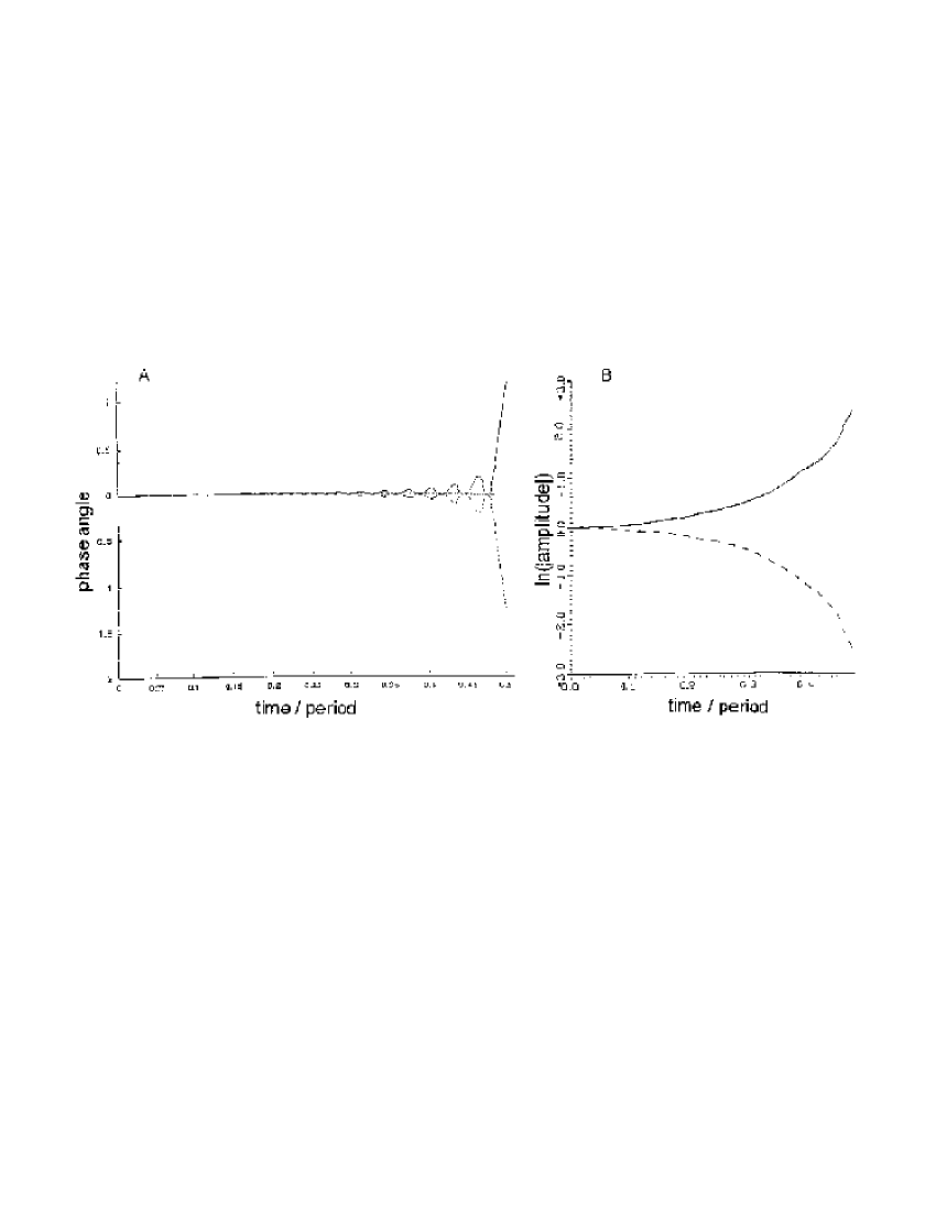
Figure 1.1: Numerical test of the reciprocal relations in equation (1.9) and equation (1.10) for $C_{g}$ shown in equation (1.29) . The values computed directly from equation (1.29) are plotted upwards and the values from the integral downwards (by broken lines) for $K/\omega=16$. The two curves are clearly identical. (a) $\ln|C_{g}(t)|$ against ($t$ /period). The modulus is an even function of $t$. (b) $\arg C_{g}(t)$ against ($t$/period). The phase is odd in $t$.

(The equality between the Fourier coefficients $A_{n}$ and $B_{n}$ was verified independently.) (b) It is a characteristic of the above two state problem (with general values of $K/\omega$), and of other problems of similar type that there is one or more roots at or near $z_{k+}=-1$ ($t=\pm\pi$; the generality of the occurrence of these roots goes back to a classic paper on conical intersection [255].) By inspection of the second sum in equation (1.49) we find that, if all the roots located in the upper half plane are of this type, then $A_{n}=B_{n}$ up to small quantities of the order of $(z_{k+}+1)$. Then again equations (1.9) and (1.10) can be employed. (c) As a corollary to the previous observation (and an important one in view of the stipulation in subsection 1.3.4, that the wave function has no real zeros) a small shift in the location of a zero originally at $t=\pm\pi$ into the complex plane either just above or just below this location, will only have a small consequence on the Fourier coefficients. Therefore, zeros of this type do not violate the assumptions of the theory. (d) If either $|z_{k+}|\gg 1$ or $|z_{k-}|\ll 1$, it is clear from equation (1.48) and equation (1.49) that the contribution of such roots is small. This circumstance is important for the following reason: Suppose that the model is changed slightly by adding to the potential a small term, e.g., adding $\epsilon\cos 2\omega t$ to a diagonal matrix element in equation (1.28) , where $\epsilon$ is small. (In [256] terms of this type were used to describe the nonlinear part of a Jahn-Teller effect.) Necessarily, this term will introduce new zeros in the amplitude. It can be shown that this addition will add new roots of the order $|z_{k+}|\approx 1/\epsilon$ or $|z_{k-}|\approx\epsilon$. The effects of these are asymptotically negligible. In other words, the formulae (1.48) and (1.49) are stable with respect to small variations in the model. [A similar result is known as Rouche’s theorem about the stability of the number of zeros in a finite domain ([265] Section 3.42).]

C. Wave packets

A time varying wave function is also obtained with a time-independent Hamiltonian by placing the system initially into a superposition of energy eigenstates ($|n>$), or forming a wave-packet. Frequently, a coordinate representation is used for the wave function which then may be written as

$$\Psi(x,t)=\sum_{m}a_{m}(t)\exp(-iE_{m}t)<x|m>$$ (1.50)

where $<x|m>$ are solutions of the time independent Schrödinger equation, with eigen-energies $E_{m}$ that are taken as non-degenerate and increasing with $m$. In this coordinate-representation, the ”component-amplitudes” in the Introduction are just fancy words for $\Psi(x,t)$ at fixed $x$ (so that the discrete state label $n$ that we have used in equation (1.8) is equivalent to the continuous variable $x$) and ($\phi_{n}(t)$ is simply $<x(t)|\Psi(x,t)>$. The results in the earlier section are applicable to the present situation. Thus, to test equation (1.9) or equation (1.10) , one would look for any fixed position $x$ in space at the moduli (or state populations) as a function of time, as with repeated state-probing set ups. In turn, by some repeated interference experiments at the same point $x$, one would establish the phase and then compare the results with those predicted by the equations. (Of course, the same equations can also be used to predict one quantity, provided the time history of the second is known.)

As in previous sections, the zeros of $\Psi(x,t)$ in the complex $t$-plane at fixed $x$ are of interest. This appears a hopeless task, but the situation is not that bleak. Thus, let us consider a wave packet initially localized in the ground state in the sense that in equation (1.50) , for some given $x$,

$$\sum_{m>0}|a_{m}<x|m>|^{2}<|a_{0}<x|0>|^{2}.$$ (1.51)

Then we expect that for such value(s) of the coordinate, the $t$- zeros of the wave-packet will be located in upper $t$-half plane only. The reason for this is similar to the reasoning that led to the theorem about the location of zeros in the near-adiabatic case. (Paragraph A, above.) Actually, empirical investigation of wave-packets appearing in the literature indicates that the expectation holds in a broader range of cases, even when the condition (1.51) is not satisfied. It should be mentioned that much of the wave packet work is numerical and it is not easy to theorize about it. (A review describing certain aspects of wave-packets is found in [257].)

We now present some examples of studied wave-packets for which the reciprocal relations hold (exactly or approximately), but have not been noted.

(a) Free-particle in one dimension.

The Hamiltonian consists only of the kinetic energy of the particle having mass $m$ ([258], [237] Section 28). The (unnormalized) energy eigenstates labeled by the momentum index $k$ are:

$$\psi_{k}(x)=\exp(ikx)$$ (1.52)

with corresponding energies $E_{k}=k^{2}/2m$. Initially the wave packet is centered on $x=0$ and has mean momentum $K$. As shown in [258], the coefficients $a_{k}$ appearing in equation (1.50) are

$$a_{k}=\exp[-(k-K)^{2}\Delta^{2}]$$ (1.53)

where $\Delta(>0)$ is the root mean square width in the initial wave packet. The expanding wave packet can be written as:

$$\ln\Psi(x,t)=-1/2\ln[\Delta+(it/2m\Delta)]-\frac{[x^{2}-4i\Delta^{2}K(x-Kt/2m)]}{[4\Delta^{2}+2it/m]}\ +\ constant$$ (1.54)

which is clearly analytic in the lower half $t$-plane. (The singularity arises because free electron wave functions are not normalizable.) We can therefore identify this function with $\ln\phi(t)=\ln\phi_{-}(t)$ in equation (1.14) , and put $\ln\phi_{+}(t)=0$. As a numerical test we have inserted equation (1.54) in equation (1.9) and equation (1.10) , integrated numerically and found (for $K=0$) precise agreement.

(b) ”Frozen Gaussian Approximation”.

Semi-analytical and semi-classical wave packets suitable for calculating evolution on an excited state multi-dimensional potential energy surface were proposed in pioneering studies by Heller [259]. In this method (called the Frozen Gaussian Approximation) the last two factors in the summand of equation (1.50) were replaced by time dependent gaussians. The time dependence arose through having time varying average energies, momenta and positions. Specifically, each coefficient $a_{m}$ in equation (1.50) was followed by a function $g(x,t)$ of the form:

$$\ln g(x,t)= - m\omega(x-<x>_{t})^{2}/2+i<p>_{t}(x-<x>_{t})$$ (1.55)

$$+ i\int_{0}^{t}(<p>_{t}^{2}/m-<g|H|g>_{t})dt$$

where $\omega$ is an energy characteristic of the upper potential surface, the angular brackets are the average position and momenta of the classical trajectory and the Dirac bracket of the Hamiltonian $H$ is to be evaluated for each component $g$ separately.

For a set of gaussians it is rather difficult to establish the analytic behavior of equation (1.55) , or of equation (1.50) , in the $t$-plane. However, with a single gaussian (in one spatial dimension) and a harmonic potential surface one has classically:

$$<x>_{t}=x_{0}\cos\omega t,$$ (1.56)

$$<p>_{t}=(m)\frac{d<x>_{t}}{dt}=-(\omega x_{0}m)\sin\omega t,$$ (1.57)

$$<g|H|g>_{t}=\omega/2$$ (1.58)

Substituting these expressions into equation (1.55) one can see after some algebra that $\ln g(x,t)$ can be identified with $\ln\chi_{-}(t)+P(t)$ shown in subsection 1.3.4. Moreover, $\ln\chi_{+}(t)=0$. It can be verified, numerically or algebraically, that the log-modulus and phase of $\ln\chi_{-}(t)$ obey the reciprocal relations (1.9) and (1.10). In more realistic cases (i.e., with several gaussians) equations (1.56)- (1.58) do not hold. It still may be true that the analytical properties of the wave packet remain valid and so do relations (1.9) and (1.10). If so, then these can be thought of as providing numerical checks on the accuracy of approximate wave-packets.

(c) Expanding waves.

As a further application we turn to the expanding potential problem ([260]-[262]), where we shall work from the amplitude-modulus to the phase. The time dependent potential is of the form:

$$V(x,t)=\zeta^{-2}(t)V(x/\zeta(t))$$ (1.59)

Here $\zeta^{2}(t)=c+t^{2}$, which differs from the more general case considered in [260]-[262], by putting their time scale factor $a=1$ and making the potential real and regular for real $t$, as well as time-inversion invariant. Then $c$ is positive and, in [260, 261] $b=0$. The Hamiltonian is singular at $t=\pm i\sqrt{c}$, away from the real axis. As first shown in [260], the generic form of the solution of the time dependent Schrödinger equation is the same for a wide range of potentials. We shall consider the ground state for a harmonic potential $V(x)=1/2m\omega_{o}^{2}x^{2}$. The log (amplitude-modulus) of the ground state wave function (in the coordinate representation) is according to [260] for real $t$

$$\ln|\phi(x,t)|=-(1/4)\ln(c+t^{2})-1/2[m\omega x^{2}/(c+t^{2})],$$ (1.60)

where $\omega^{2}=\omega_{o}^{2}+c$. Processing the expression in equation (1.60) as in equation (1.14) , we can arbitrarily decompose $\phi(x,t)$ into factors that are analytic above and below the real $t$-axis. Thus, let us suppose that in equation (1.60) a fraction $f_{1}$ of the first term and a fraction $f_{2}$ of the second term is analytic in the upper half and, correspondingly, fractions $(1-f_{1})$ and $(1-f_{2})$ are analytic in the lower half. Explicitly, for complex $t$

$$\ln|\phi(x,t)| = Re\ \{-1/2[f_{1}\ln(\sqrt{c}-it)+(1-f_{1})\log(\sqrt{c}+it)]$$ (1.61)

$$- 1/2(m\omega x^{2}/\sqrt{c})[f_{2}/(\sqrt{c}-it)$$

$$+ (1-f_{2})/(\sqrt{c}+it)]\}.$$

Next, for the log term (which normalizes the wave function), we have to choose, as in equation (1.15) , suitable functions $P_{\pm}(t)$ that will ”correct” the behavior of that term along the large semi-circles. Among the multiplicity of choices the following are the most rewarding (since they completely cancel the log term):

$$P_{+}(t) = -f_{1}(1/2)\ln(\sqrt{c}-it)$$

$$= -(f_{1}/4)[\ln(t^{2}+c)-2i\arctan(t/\sqrt{c})],$$

$$P_{-}(t) = -(1-f_{1})(1/2)\log(\sqrt{c}+it)$$

$$= -(1/4)(1-f_{1})[\ln(t^{2}+c)+2i\arctan(t/\sqrt{c})].$$

The right hand side of equation (1.18) comes from the second term of equation (1.60) alone and is

$$\arg\chi(x,t)=(1-2f_{2})[m\omega x^{2}/(t^{2}+c)](t/4\sqrt{c}).$$ (1.62)

To complete the phase of the wave function, $\arg\phi(x,t)$, we have to reinstate the terms $P_{\pm}(t)$ that were removed in equation (1.15) so as to get $\chi_{\pm}(x,t)$. The result is:

$$\arg\phi(x,t)=-(1-2f_{1})(1/2)\arctan(t/\sqrt{c})+(1-2f_{2})[m\omega x^{2}/(t^{2}+c)](t/4\sqrt{c})$$ (1.63)

This establishes the functional form of the phase for real (physical) times. The phase of the solution given in [260, 261] has indeed this functional form. The fractions $f_{1}$ and $f_{2}$ cannot be determined from our equations (1.17) and (1.18). However, by comparing with the wave functions in [260, 261], we get for them the following values.

$$1-2f_{1}=\omega/\sqrt{c},\qquad 1-2f_{2}=4\sqrt{c}/\omega$$ (1.64)

In the excited states for the same potential, the log modulus contains higher order terms in $x$ ($x^{3}$, $x^{4}$, etc.) with coefficients that depend on time. Each term can again be decomposed (arbitrarily) into parts analytic in the $t$-half-planes, but from elementary inspection of the solutions in [260, 261] it turns out that every term except the lowest (shown in equation (1.59) ) splits up equally (i.e. the $f$’s are just $1/2$) and there is no contribution to the phases from these terms. Potentials other than the harmonic can be treated in essentially identical ways.

1.3.6 Consequences

The following theoretical consequences of the reciprocal relations can be noted:

(i) They unfold a connection between parts of time-dependent wave functions that arises from the structure of the defining equation (1.2) and some simple properties of the Hamiltonian.

(ii) The connection holds separately for the coefficient of each state component in the wave function and is not a property of the total wave function (as is, e.g., the ”dynamical” phase [9]).

(iii) The relations pertain to the fine, small-scale time-variations in the phase and the log modulus, not to their large scale changes.

(iv) One can define a phase that is given as an integral over the log of the amplitude modulus and is therefore an observable and is gauge-invariant. This phase (which is unique, at least in the cases for which equation (1.9) holds) differs from other phases, those that are, e.g. a constant, the dynamic phase or a gauge-transformation induced phase, by its satisfying the analyticity requirements laid out in subsection 1.3.3.

(v) Experimentally, phases can be obtained by measurements of occupation probabilities of states using equation (1.9) . (We have calculationally verified this for the case treated in [263].)

(vi) Conversely, the implication of equation (1.10) is that a geometrical phase appearing on the left-hand-side entails a corresponding geometric probability change, as shown on the right-hand-side. Geometrical decay probabilities have been predicted in [161] and experimentally tested in [264].

(vii) An important ingredient in the analysis has been the positions of zeros of $\Psi(x,t)$ in the complex t-plane for a fixed x. Within quantum mechanics the zeros have not been given much attention, but they have been studied in a mathematical context [265] and in some classical wave-phenomena ([266] and references cited therein). Their relevance to our study is evident since at its zeros the phase of $\Psi(x,t)$ lacks definition. Future theoretical work shall focus on a systematic description of the location of zeros. Further, practically oriented work will seek out computed or experimentally acquired time dependent wave functions for tests or application of the present results.

(viii) Finally, and probably most importantly, the relations show that changes (of a nontrivial type) in the phase imply necessarily a change in the occupation number of the state components and vice versa. This means that for time-reversal-invariant situations, there is (at least) one partner state with which the phase-varying state communicates.

1.4 Non-Linearities That Lead to Multiple Degeneracies

In previous sections of this review we have treated molecules and other localized systems in which a linear electron-nuclear coupling resulted in a single degeneracy, or conical intersection (ci) of the electronic potential energy surfaces. A notable, symmetry-caused example of this is the linear $E\otimes\epsilon$ Jahn-Teller effect (a pair of degenerate electronic states, that can happen under trigonal or higher symmetry, which is coupled to two energetically degenerate displacement modes) [267, 156, 47]. Still, some time ago nonlinear coupling was also considered within the $E\otimes\epsilon$ case in [268, 269] and subsequently in [256]. Such coupling can result in a more complex situation, in which there is a quadruplet of ci’s, such that one ci is situated at the origin of the mode coordinates (as before) and three further ci’s are located farther outside in the plane, at points that possess trigonal symmetry.

As of late, non-linear coupling has become of increased interest, partly through evidence for a weak linear coupling in the metallic cluster $Na_{3}$ [53, 270] (computations of vibrational levels in a related molecule $Li_{3}$ were performed in [271, 272]), and partly by attempts to computationally locate ci’s in the potential energy landscape with a view to estimate their effect on inter-surface, non-adiabatic transitions [273]. The method used in the last reference was based on the acquisition of the geometric phase by the total function as a ci is circled [274, 157, 158, 9]. Independently, the authors of [55] found theoretically a causal connection between the number of ci effectively circled (one or four) and the important question of the nature of the ground state. They showed that, contrary to what had been widely thought before, the ground state may be either a vibronic doublet or a singlet, depending on the distance (which is a function of the parameters in the vibronic Hamiltonian) of these trigonal ci’s from the centre. (A similar instance of ”quantum phase transition” was noted for a threefold degenerate system in [275] and, earlier, for an icosahedral system, in [276]).

In a different field, location and characteristics of ci’s on diabatic potential surfaces have been recognized as essential for the evaluation of dynamic parameters, like non-adiabatic coupling terms, needed for the dynamic and static properties of some molecules ([277] -[280], [192]). More recently, pairs of ci’s have been studied [281, 282] in greater detail. These studies arose originally in connection with a ci between the $1^{2}A^{\prime}$ and $2^{2}A^{\prime}$ states found earlier in computed potential energy surfaces for $C_{2}H$ in $C_{s}$ symmetry [278]. Similar ci’s appear between the potential surfaces of the two lowest excited states ${}^{1}A_{2}$ and ${}^{1}B_{2}$ in $H_{2}S$ or of ${}^{2}B_{2}$ and ${}^{2}A_{1}$ in $Al-H_{2}$ within $C_{2v}$ symmetry [283]. A further, closely spaced pair of ci’s has also been found between the $3^{2}A^{\prime}$ and $4^{2}A^{\prime}$ states of the molecule $C_{2}H$. Here the separation between the twins varies with the assumed $C-C$ separation, and they can be brought into coincidence at some separation [282].

In this section we investigate the phase changes that characterize the double and trigonal (or cubic) ci’s. We shall find that the Berry phases upon circling around the ci’s can take the values of $0$ or $2N\pi$ (where $N$ is an integer). It can be shown that the different values of $N$ can be made experimentally observable (through probing the state populations after inducing changes in the amplitudes of the components), in a way that is not marred by the fast oscillating dynamic phase. Apart from the results regarding the integer $N$ in the Berry phase, the difference between our approach to the phase changes and those in some previous works, especially in [283, 273], needs to be noted. While these consider the topological phase belonging to the total wave packet, we continue in the spirit of the previous section 3 and treat the open phase belonging to a single component of the wave packet. (For the topological, full-cycle phase the two are equivalent, but not for the open phase, that is present at interim stages.) Explicitly, we write the (in general) time ($t$)-dependent molecular wave function $\Psi(t)$ as a superposition of (diabatic) electronic states $\chi_{k}$ as

$$\Psi(t)=\sum_{k}a_{k}(t)\chi_{k}$$ (1.65)

where the amplitudes $a_{k}$ are functions of the nuclear coordinates. In the previous section we have developed and used the reciprocal relations between the phases ($arg\ a_{k}$) and the (”observable”) moduli ($|a_{k}|$).

We also describe a ”tracing” method to obtain the phases after a full cycling. We shall further consider wave-functions whose phases at the completion of cycling differ by integer multiples of $2\pi$ (a situation that will be written, for brevity, as ”$2N\pi$ ”). Some time ago, these wave functions have been shown to be completely equivalent, since only the phase factor (viz., $e^{iPhase}$ ) is observable [155]; however, this is true only for a set of measurements that are all made at instances where the phase difference is $2N\pi$. We point out simple, necessary connections between having a certain $2N\pi$ situation and observations made prior to the achievement of that situation. The phase that is of interest in this review is the Berry phase of the wave-function [9], not its total phase, though this distinction will not be re-stated.

1.4.1 Conical Intersection Pairs

We treat this case first, since it is simpler than the trigonal case. The molecular displacements are denoted by $x$ and $y$ (with suitable choice of their origins and of scaling). Then, without loss of generality we can denote the positions of the ci pairs in Cartesian coordinates by

$$x=\pm 1,\qquad y=0$$ (1.66)

or, in polar coordinates, where $x=q\cos\phi$, $y=q\sin\phi$, by

$$q=1,\qquad\phi=0,\pi$$ (1.67)

To obtain potential surfaces for two electronic states which will be degenerate at these points, we write a Hamiltonian as a 2x2 matrix in a diabatic representation in the following form:

$$H(x,y) = K\left(\begin{array}[]{cc}-(x^{2}-1)&yf(x)\\ yf(x)&(x^{2}-1)\end{array}\right)$$ (1.70)

$$= K\left(\begin{array}[]{cc}-(q^{2}\cos^{2}\phi-1)&q\sin\phi f(q\cos\phi)\\ q\sin\phi f(q\cos\phi)&(q^{2}\cos^{2}\phi-1)\end{array}\right)=H(q,\phi)$$ (1.73)

whose two eigenvalues are

$$E_{\pm}(x,y) = \pm K\sqrt{(x^{2}-1)^{2}+[yf(x)]^{2}}$$ (1.74)

$$= \pm K\sqrt{(q^{2}\cos^{2}\phi-1)^{2}+[q\sin\phi f(q\cos\phi)]^{2}}$$

$$= E_{\pm}(q,\phi)$$

For $K$ a (positive) constant and $f(x)$ a function which is non zero at $x=\pm 1$, the Hamiltonian in equation (1.73) can be taken as a model that yields the postulated ci pairs, since the two eigenvalues coincide just at the points given by equation (1.66) or equation (1.67) . There may be more general models that give the same two ci’s. (Note, however, that if $f(x)$ had a zero at $x=\pm 1$, the degeneracy of energies would not be conical.) We now make the above model more specialized and show that different values of the Berry phase can be obtained for different choices of $f(x)$. For definiteness we consider specific molecular situations, but these are just instances of wider categories. (The notation of Herzberg [284] is used.)

$1A_{1}$ and $2A_{2}$ states in $C_{2v}$ symmetry (Exemplified by ${}^{1}A_{1}^{(1)}$ and ${}^{1}A_{1}^{(2)}$ in bent $HCH$.)

If the $x$ coordinate represents a mode displacement that transforms as $B_{1}$ (e.g., an asymmetric stretch of $CH$) and $y$ transforms as $A_{1}$ (a flapping motion of the $H_{2}$, this coordinate being the same as $y$ in figure 169 of [284]), then $f(x)$ in equation (1.73) can be taken as a constant. Without loss of generality we put for this case $f(x)=1$ and find that cycling adiabatically counterclockwise around the ${\it ci}$ that is at $(-1,0)$ induces (in the component that is unity at $\phi=0$) a topological phase of $\pi$, and that around $(1,0)$ yields $-\pi$. Cycling either fully inside or outside $q=1$ (the latter case encircling both ci’s), gives zero phase. We now describe a ”continuous (phase-) tracing method” that obtains in an unambiguous way the phase of a real wave function. The alternative, ”adiabatic cycling” method of the previous section gave the same phase change in terms of the evolution of the complex solution of the time dependent Schrödinger equation in the extremely slow (adiabatic) limit. Other methods will be briefly referred to.

1.4.2 Continuous Tracing of the Component Phase

In this method one notes that real-valued solutions of the time independent Hamiltonian of a $2\times 2$ matrix form can be written in terms of an $\theta(\phi,q)$, which is twice the ”mixing angle”, such that the electronic component which is ”initially” $1$ is $\cos[\theta(\phi,q)/2]$, while that which is initially $0$ is $\sin[\theta(\phi,q)/2]$. For the second matrix form in equation (1.73) (in which, for simplicity $f(x)=1$), we get

$$\theta(\phi,q)=\arctan\frac{q\sin\phi}{q^{2}\cos^{2}\phi\ -1}$$ (1.75)

One can trace the continuous evolution of $\theta$ (or of $\frac{\theta}{2}$) as $\phi$ describes the circle $q=constant$. This will yield the topological phase (as well as intermediate, open-path phase during the circling). We illustrate this in the next two figures for the case $q>1$ (encircling the ${\it ci}$’s).

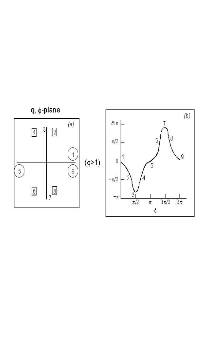
Figure 1.2: Phase-tracing for the case of $1A_{1}$ and $2A_{2}$ states in $C_{2v}$ symmetry: (a) The left-hand side shows the labels for the significant stages during the circling in the $(q,\phi)$-plane. In this and the following figures, numbers in circles represent the positions of zeros in the argument of the arctan in the expression of the angle, (equation (1.75) ), numbers in squares are poles and free numbers are other significant stages in the circling. (b) The angle $\theta$ in equation (1.75) as function of the circling angle. The numbers correspond to those on the adjacent part (a) of the figure. (Note: The angle $\theta$ is defined as twice the transformation or mixing angle.) The circling is with $q>1$, namely outside the ci pair.

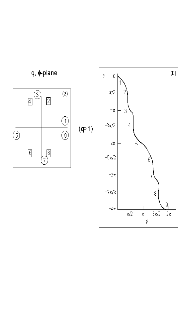
Figure 1.3: Phase-tracing for circling outside the ci pair (for the model in $A_{1}$ and $B_{2}$ states in $C_{2v}$ symmetry. The Berry phase (half the angle shown at the extremity of the figure) is here $-2\pi$.

Figure 1.4: Probabilities in different models during adiabatic circling around ci’s. The square moduli of component amplitudes as function of time are seen to be different for different models. Long-dashed lines: the model in $1A_{1}$ and $2A_{2}$ states in $C_{2v}$ symmetry for circling inside the ci’s. Full lines: the model in $1A_{1}$ and $2A_{2}$ states in $C_{2v}$ symmetry for circling outside the ci’s. Broken lines: the model in $A_{1}$ and $B_{2}$ states in $C_{2v}$ symmetry (with the ”$xy$” off-diagonal matrix element) for circling outside the ci’s. In the latter model, circling inside the ci’s gives probabilities that would be indistinguishable from unity on the figure (and are not shown).

In the sub-figure (1.2.a) several important stages in the circling are labeled with Arabic numerals. In the adjacent sub-figure (1.2.b) the values of $\theta(\phi,q)$ are plotted as $\phi$ increases continuously. The labeled points in the two sub-figures correspond to each other. (The notation is that points which represent zeros of $\tan\theta$ are marked with numbers surrounded by small circles, those which represent poles are marked by numbers placed inside squares, other points of interests that are neither zero nor poles are labeled by free numbers.) The zero value of the topological phase ($\frac{\theta}{2}$) arises from the fact that at the point $2$ (at which ${\it\phi}$ =$\frac{\pi}{2}$), $\theta$ retraces its values, rather than goes on to decrease.

$A_{1}$ and $B_{2}$ states in $C_{2v}$ symmetry (Exemplified by ${}^{2}A_{1}$ and ${}^{2}B_{2}$ in $AlH_{2}$ [285])

Symmetry considerations forbid any non-zero off-diagonal matrix elements in equation (1.73) when $f(x)$ is even in $x$, but they can be non-zero if $f(x)$ is odd, e.g., $f(x)=x$. (We note that $x$ itself transforms as $B_{2}$ [284].) Figure 1.3 shows the outcome for the phase by the continuous phase tracing method for cycling outside the ci’s ($q>1$). The difference between the present case and the previous one (in which $f(x)$ was an even function of $x$) is that now, in the second half of circling in the $q,\ \phi$ - plane, the wave-function component angle $\theta$ does not retrace its path, but goes on decreasing. (It is interesting to remark here on an analogy between the present results and the well known results of contour integration in the complex $z$ - plane. An integration of $(z^{2}-1)^{-1}$ over a path that encircles the two poles of the function gives zero result, but the same path integration of $z(z^{2}-1)^{-1}$, gives $2\pi i$. However, the analogy does not work fully. Thus, a simple multiplication of the integrand by a positive constant alters the residues, but not the phase.)

However, the resulting Berry phase of $-2\pi$ depends on (i) having reached the adiabatic limit and (ii) circling well away from the ci’s; i.e., it is necessary that the circling shall be done with a value of $q$ that is either much smaller or much larger than $1$. A contrary case not satisfying these conditions, e.g., when either $q<3$ or $K<60$ , would give a Berry phase of about $4\pi$, $6\pi$, $\ldots$, or a number $N\approx 2,3,\ldots$ rather than $1$, as might have been expected. What is perhaps remarkable is that even in the not quite adiabatic or not very large $q$ cases, $N$ (though plainly different from $1$) is still close to being an integer. More study may be needed on this result, especially in view of the possibility of observable consequences of the value of $N$. The cases of ”$1A_{1}$ and $2A_{2}$ states in $C_{2v}$ symmetry” and of ”$A_{1}$ and $B_{2}$ states in $C_{2v}$ symmetry” are, of course, inequivalent, since they arise from different Hamiltonians. Their non equivalence results not only in different topological phases (zero and $2\pi$), but in different state occupation probabilities. These are defined as the probabilities of the systems being in one of the states $\chi_{k}$, of which the superposition in equation (1.65) is made up. In Figure 1.4 we show these probabilities as functions of time for systems that differ by their having different functions $f(x)$ in the off-diagonal positions of the Hamiltonian. The differences in the probabilities are apparent.

Trigonal Degeneracies

The simplest way to write down the 2-by-2 Hamiltonian for two states such that its eigenvalues coincide at trigonally symmetric points in $(x,y)$- or $(q,\phi)$ -plane is to consider the matrices of vibrational-electronic coupling of the $E\otimes\epsilon$ Jahn-Teller problem in a diabatic electronic state representation. These have been constructed by B. Halperin, and listed in Appendix IV of [156], up to the third order in $q$. The first order or linear coupling in the displacement coordinates is of the well known form (shown by the first term in the Hamiltonian presented below) and yields the familiar ci at the origin, $q=0$. When one adds to this the quadratic coupling, designated $I(E)$ in section IV.3 (A) of the above reference and quoted below, one obtains three further, trigonally situated ci, namely at either $\phi=0,\pm\frac{2\pi}{3}$, or $\phi=\pi,\pm\frac{4\pi}{3}$, depending on whether the signs of the linear and quadratic couplings are the same or opposite. The distance of the trigonal ci’s from the origin varies with the relative magnitudes of the couplings: the higher the strength of the quadratic term, the nearer the trigonal ci are to the center. This was, of course, the physical basis of [55], in which a ground vibronic singlet state for strong quadratic coupling was found. The resulting Hamiltonian is of the form (to be compared with the two matrices in equation (1.73) above):

$$H(x,y) = K\left(\begin{array}[]{cc}-(x-2\kappa(x^{2}-y^{2}))&y+4\kappa xy\\ y+4\kappa xy&(x-2\kappa(x^{2}-y^{2}))\end{array}\right)$$ (1.78)

$$= K\left(\begin{array}[]{cc}-(q\cos\phi-2\kappa q^{2}\cos 2\phi)&q\sin\phi+2\kappa q^{2}\sin 2\phi\\ q\sin\phi+2\kappa q^{2}\sin 2\phi&(q\cos\phi-2\kappa q^{2}\cos 2\phi)\end{array}\right)$$ (1.81)

$$= H(q,\phi)$$ (1.82)

where $\kappa$ represents the ratio of the strength of the quadratic coupling to the linear one. The trigonal ci ’s are at a distance $q=(2\kappa)^{-1}$, with angular positions as described above. Employing now the continuous phase tracing method introduced in subsection 1.4.1, one again obtains the graphs for the mixing angle. There are now three cases to consider, namely (i) for cycling that encloses all four ci’s , ($q>(2\kappa)^{-1}$) the resulting phase acquired being now $2\pi$ (shown in Fig. 1.5)

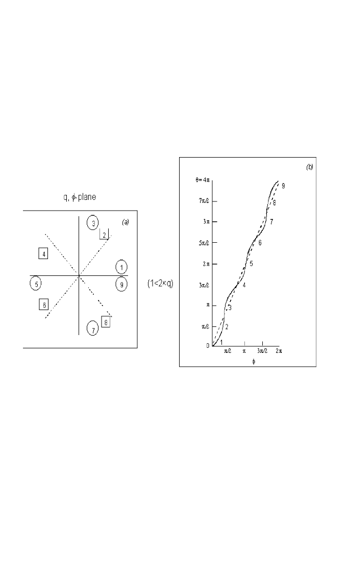
Figure 1.5: Phase-tracing for the case of trigonal degeneracies when the circle encompasses all four ci’s and the Berry phase is $2\pi$.

This is an even multiple of $\pi$, as expected for four ci’s [274], but differs from $4\pi$ (or from zero). Then (ii) for intermediate radius cycling ($(2\kappa)^{-1}>q>(4\kappa)^{-1}$) (which is shown in Fig. 1.6)

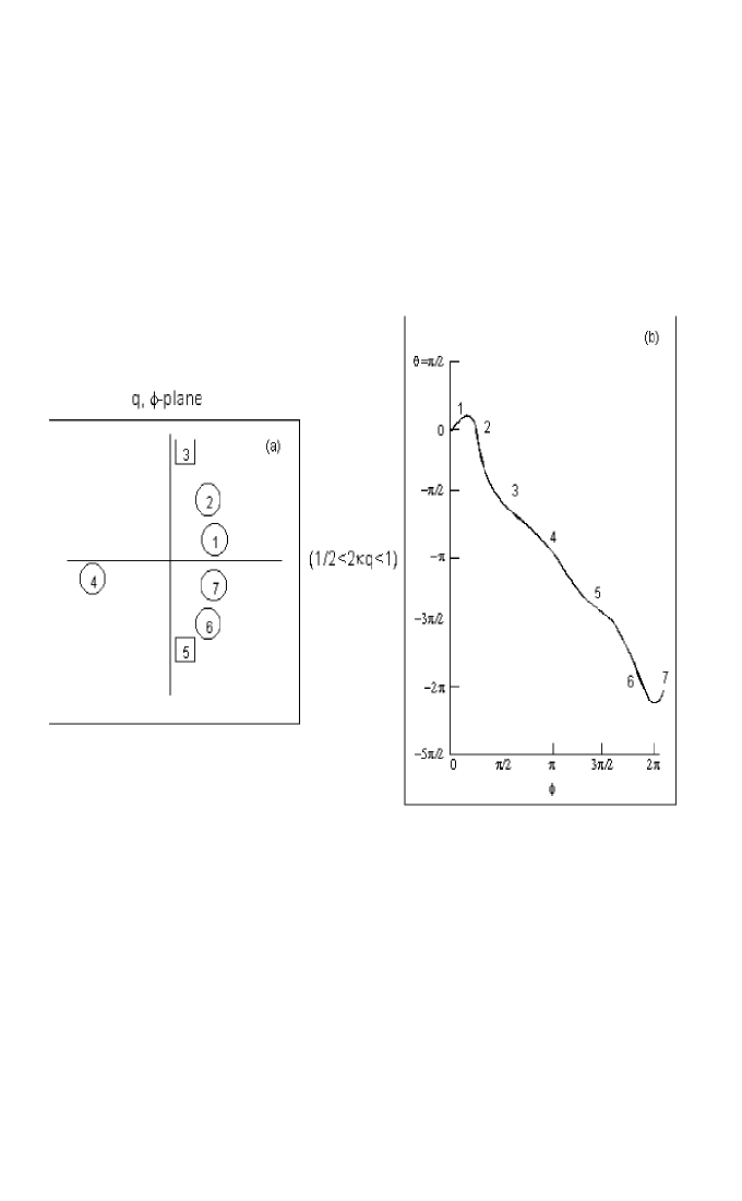
Figure 1.6: Phase-tracing for the trigonal degeneracies. The drawings (which are explained in the caption to figure 1.3) are for intermediate-radius ($q$) circling.

that terminates with a Berry phase of $-\pi$, and lastly (iii) for small radius cycling $(q<(2\kappa)^{-1})$. The last case has also the Berry phase of $\pi$ , but differs from the intermediate case (ii), in that the initial increase is absent.

It might be asked what happens when one adds further couplings beyond the quadratic one? In the next higher order one finds a scalar cubic term of the form:

$$q^{3}cos3\pi\bf I$$ (1.83)

where $\bf I$ is the unit matrix. This gives rise to three trigonally aligned degeneracies ([156], Appendix IV). However, these are parabolic (touching) degeneracies, not conical intersections, and do not cause changes of sign in the wave function upon circling round them. Higher order terms (not listed in that Appendix) can give rise to additional ci ’s of trigonal symmetry, but the strength of these terms is expected to be less and therefore the resulting ci’s will be farther outside, where are without importance for low lying states. Still, their presence is of interest for revealing the connection between the Berry angle and the number of ci’s circled and we shall presently obtain nonlinear coupling terms to an arbitrarily high power of $q$.

1.4.3 The Adiabatic to Diabatic Transformation (ADT)

Several years ago Baer proposed the use of a matrix $A$, that transforms the adiabatic electronic set to a diabatic one [48]. (For a special two-fold set this was discussed in [286, 287].) Computations performed with the diabatic set are much simpler than those with the adiabatic set. Subject to certain conditions, $A$ is the solution of a set of first order partial differential equations. $A$ is unitary and has the form of a ”path-ordered” phase factor, in which the phase can be formally written as

$$\int_{\bf{R_{0}}}^{\bf R}\bf f^{IJ}(\bf R)\cdot d{\bf R}$$ (1.84)

Here the integrand is the off-diagonal gradient matrix element between adiabatic electronic states,

$$\bf f^{IJ}(\bf R)=<I|\vec{\nabla}|J>$$ (1.85)

($\vec{\nabla}$ is the derivative with respect to $\bf R$.) We stress that in this formalism, $I$ and $J$ denote the complete adiabatic electronic state, and not a component thereof. $|I>$ and $|J>$ contain the nuclear coordinates, designated by ${\bf R}$, as parameters. The above line integral was used and elaborated in calculations of nuclear dynamics on potential surfaces by several authors ([273, 283], ([288] -[301]). (For an extended discussion of this and related matters the reviews of Sidis [49] and Pacher et al. [50] are especially informative.)

The possibility of a non-gradient component in the integrand introduces some difficulty and an alternative formulation has been proposed [283, 273]. (At positions that are close to a ci, the alternative approximates well to the angle shown above in equation (1.84) .)

The ADT, computed for $\it ci$ pairs in [57] and denoted (in their figures 1-3) by $\gamma(\phi|q)$, is related to the ”open path phase” defined below in equation (1.86) , but is identical with it (and with Berry’s angle) only at $\phi=2\pi$. At this value the computed results of [57] are in agreement with those that were derived with the model Hamiltonian in equation (1.73) . However, in some of the cases, when the coupling terms became zero, the sign that the phase $\gamma(\phi|q)$ acquires might become ambiguous (e.g., whether it is even or odd under reflection about the line $\phi=\pi$). In the above analytic models the signs are given unambiguously.

Since up to date summaries about the practical implementation of the line integral have been given recently (in [282, 108]; as also in the chapter by Baer in the present volume), and the method was applied also to a pair of ci’s [282], we do not elaborate here on the form of the phase associated with one or more ci’s, as obtained through this method .

1.4.4 Direct Integration

The open path phase [14, 11] associated with a component- amplitude can be obtained as the imaginary part of an integral:

$$\gamma_{k}(t)=Im\ \int_{0}^{t}dt^{\prime}\frac{\partial a_{k}(t^{\prime})}{\partial t^{\prime}}/a_{k}(t^{\prime})$$ (1.86)

where, as before at several places in this chapter, $a_{k}(t)$ is the amplitude of the $k$-component in the solution of the time - dependent Schrödinger equation in the near- adiabatic limit. The (complex) amplitude in the integrand is (in general) non-vanishing (unlike the real wave-function amplitude in the strictly adiabatic solution) and thus the integral is non-divergent. However, in practice, even fairly close to the adiabatic limit, the convergence is very slow, due to oscillations in the amplitude, noted in the previous section and in [29]-[32]. For this reason, the formula in equation (1.86) is not a convenient one to use. Still, using the formula for increasing values of the adiabaticity parameter (i.e. increasing $K$ in equation (1.73) to $K>10^{2}$), we have evaluated the topological phase for the case with trigonal symmetry and have found it to converge close to the value $2N\pi$, with N=1 (and not 0). Because of the diffiulties in its practical implementation, we shall not further consider the direct integration method.

1.4.5 Higher Order Coupling in some Jahn-Teller and Renner-Teller Effects

A systematic derivation of forms of coupling that is super-linear in the nuclear motion amplitude was given, partly based on Racah coefficients, in [156], Appendix IV, but these went up only as far as the third order in the amplitudes $q$. As will shortly be made apparent, there is some theoretical need to obtain higher order terms. For the $E\otimes\epsilon$ Jahn-Teller case, the form of coupling to arbitrary powers was given in [302]. Here we give a different and arguably simpler derivation using the vector-coupling formalism of Appendix IV in [156], the complex representation form given in [303], and a mathematical induction type of argument.

Complex Representation

The mode coordinates, transforming respectively as the $-1$ and $1$ components of the $E$ (doubly degenerate) modes, have the form:

$$(g_{-1},g_{1})=-(i/\sqrt{2})(g_{\theta},g_{\epsilon})\left(\begin{array}[]{cc}-1&1\\ \ i&i\end{array}\right)=(i/\sqrt{2})(qe^{-i\phi},-qe^{i\phi})$$ (1.87)

where the extreme right-hand member recalls the ”modulus” $q$ and the ”phase” $\phi$ used in the real representation. The vector coupling -coefficients for e.g. octahedral symmetry, can be obtained from Table A.20 in the Appendix 2 of [304], upon performing the transformation shown (1.87) on the real representation. In the following Table we show the Clebsch-Gordan coefficients defined in equation (1.90) below.

A:	B:		C:	$A_{1}$	$A_{2}$	E
E	E		–	–	–	–	–
a:	b:		c:	$a_{1}$	$a_{2}$	1	1
		U:	–	–	–	–	–
1	1			0	0	-i	0
1	-1			$1/\sqrt{2}$	$-i/\sqrt{2}$	0	0
-1	1			$1/\sqrt{2}$	$i/\sqrt{2}$	0	0
-1	-1			0	0	0	1

Table 1.1: The coupling- coefficients $U(ABC|abc)$ for the complex form of a doubly degenerate representation, following G.F. Koster et al ”Properties of the thirty-two point groups” (MIT Press, Cambridge, Mass., 1963), pp. 8, 52.

To obtain non-linear coupling terms, we consider two linearly independent, not identical $E$-modes, namely

$$(g_{-1},g_{1})$$ (1.88)

$$(G_{-1},G_{1})$$ (1.89)

and construct bilinear expressions from these. The combination that transforms as components of an $E$-mode is given by

$$\chi(E|x)=\sum_{a,b}U(EEE|abx)g_{a}G_{b}$$ (1.90)

The above Table for U immediately shows that there are only two bilinear combinations of $g$ and $G$, namely those $a=1$, $b=1$ and $a=-1$, $b=-1$. These lead to the quadratic terms belonging to the components $-1$ and $1$: $\chi(E|-1)=g_{1}G_{1}$ and $\chi(E|1)=g_{-1}G_{-1}$

Eq. A IV.4 of [156] tells us which ket-bra operator $|d><e|$ is multiplied by the above combinations or, equivalently, where in the $2\times 2$ electronic- nuclear coupling matrix each of these terms sit. Here again we adopt for the electronic kets a complex representation, analogous to that shown in equation (1.87) . To use the vector coupling coefficients for these, we recall that in the complex representation the bra’s transform as the corresponding ”minus-label ket”’s (cf. Eq. (2.34) in [303]). Using again the vector coupling coefficients, we see that $\chi(E|-1)$ is the factor that multiplies $|1><-1|$ (and $\chi(E|1)$ is the factor that multiplies $|-1><1|$). In the usual matrix notation [in which rows and columns are taken in the order $(-1,1)$] this means that in the upper right corner one has (for linear coupling ) $g_{-1}$ and $G_{-1}$, and (for quadratic coupling), $g_{1}G_{1}$, and similarly in the lower left corner $g_{1}$, $G_{1}$ , as well as $g_{-1}G_{-1}$. Both linear and quadratic terms will be multiplied by different constants, whose values depend on the physical situation and cannot be given by symmetry considerations, except that the electronic- nuclear interaction must be Hermitean and invariant under the symmetry operations of the group. The same construction can be employed to derive bilinear terms on the diagonal part of the coupling matrix. Using again the $U$-coefficients in the Table, one obtains the forms (not normalized)

$$(g_{1}G_{-1}+g_{-1}G_{1})(|1><1|+|-1><-1|)$$ (1.91)

where each factor belongs to the $A_{1}$ representation and

$$(g_{1}G_{-1}-g_{-1}G_{1})(|1><1|-|-1><-1|)$$ (1.92)

where each factor belongs to the $A_{2}$ representation.

Squaring of Off-diagonal Elements

The method shown affords easy generalization to higher order coupling in the important case where a single mode is engaged, i.e., $G_{\pm 1}=g_{\pm 1}=\pm\frac{1}{i\sqrt{2}}qe^{\pm i\phi}$. Then the two off-diagonal terms derived above are, after physics based constant coefficients have been affixed, in the upper right corner

$$(qe^{-i\phi}-2\kappa q^{2}e^{2i\phi})|1><-1|$$ (1.93)

with another, Hermitean conjugate expression on the other (lower left) off-diagonal position. These were previously given in a similar form in, e.g., [256, 156]. The $A_{1}$ term in equation (1.91) only renormalizes the vibrational frequency. The $A_{2}$ term vanishes (for terms up to second order in $q^{2}$). Proceeding in the same way to get further terms by cross multiplying the second order expression in equation (1.93) , and continuing the procedure, we obtain in the upper right corner the following terms correct up to the fourth order in $q$:

$$q^{3}e^{-i\phi},q^{4}e^{2i\phi},q^{4}e^{-4i\phi}$$ (1.94)

The first and second terms contain phase factors identical to those previously met with in equation (1.93) . The last term has the ”new” phase factor $e^{-4i\phi}$ (Though the power of $q$ in the second term is different from that in equation (1.93) , this term enters with a physics-based coefficient that is independent of $\kappa$ in equation (1.93) , and can be taken for the present illustration as zero. The full expression is shown below in equation (1.97) and the implications of higher powers of $q$ are discussed thereafter.) Then a new off-diagonal matrix element enlarged with the third term only, multiplied by a (new) coefficient $\lambda$, is

$$(qe^{-i\phi}-2\kappa q^{2}e^{2i\phi}+\lambda q^{4}e^{-4i\phi})=qe^{-i\phi}(1-2\kappa qe^{3i\phi}+\lambda q^{3}e^{-3i\phi})$$ (1.95)

There is going to be an $A_{1}$ (scalar) term of the form, well known in the literature (e.g., [156]), $q^{3}\cos 3\phi$, and an $A_{2}$ (pseudo- scalar) term of the form $q^{3}\sin 3\phi$. We may once again suppose that the coefficients of all these terms are independent (i.e., their physical origins are different) and that we may discuss terms in diagonal and off-diagonal positions separately. Let us consider the off-diagonal term, as given on the right hand member of equation (1.95) . The vanishing of the first factor gives the traditional conical intersection (ci) at the origin. The zeros of the second factor give additional ci’s. These are all trigonally positioned, due to the phase factors $e^{\pm 3i\phi}$, which induce trigonal symmetry. The maximum number of trigonal ci’s (to this, fourth order approximation in q) is clearly $3\times 3=9$. Thus, to give a numerical example in which $\kappa=0.15$, $\lambda=0.003$, we obtain the following nine trigonal roots of equation (1.95)

$$q=3.95, \phi=0,\frac{2\pi}{3},\frac{4\pi}{3}$$ (1.96)

$$q=7.42, \phi=0,\frac{2\pi}{3},\frac{4\pi}{3}$$

$$q=11.37, \phi=\pi,\frac{\pi}{3},\frac{5\pi}{3}$$

(Clearly the pseudo-scalar term vanishes at these points; so the ci character at the roots is maintained, no matter whether there are or are not $A_{2}$ terms. Also the vanishing of $A_{2}$ terms will not lead to new ci’s.) On the other hand, by circling over a large radius path $q\rightarrow\infty$, so that all ci’s are enclosed, the dominant term in equation (1.95) is the last one and the acquired Berry- phase is $-4(2\pi)/2=-4\pi$.

To see that this phase has no relation to the number of ci’s encircled (if this statement is not already obvious), we note that this last result is true no matter what are the values of the coefficients $\kappa$ , $\lambda$, etc., provided only that the latter is non-zero. In contrast, the number of ci’s depends on their values; e.g. for some values of the parameters the vanishing of the off-diagonal matrix elements occurs for complex values of $q$, and these do not represent physical ci’s. The model used in [270] represents a special case, in which it was possible to derive a relation between the number of ci’s and the Berry- phase acquired upon circling about them. We are concerned with more general situations. For these it is not warranted, for example, to count up the total number of ci’s by circling with a large radius.

General Off-diagonal Coupling

The construction given above to obtain off-diagonal non-linear couplings up to order $q^{4}$ can be generalized to arbitrary order. Only the final result is given. This gives for the off diagonal term in the upper right corner:

$$Kqe^{-i\phi}[1+q^{-2}\sum_{m=1,\ldots}q^{3m}Q_{m+}e^{3mi\phi}+\sum_{m=1,\ldots}q^{3m}Q_{m-}e^{-3mi\phi}]$$ (1.97)

where $Q_{m+}$ and $Q_{m-}$ are polynomials in $q^{2}$ with coefficients that depend on the physical system and whose leading terms will be $q^{0}$ . When transformed back to the real representation, by applying the inverse of the transformation in equation (1.87) , one regains the expressions of [302]. Normally, for stable physical systems, it is expected that, with increasing $m$ , $Q_{m+}$ and $Q_{m-}$ will numerically decrease and so will, in each polynomial, the coefficients of successively higher powers $q^{2}$. If we assume only a finite number of summands in the above sums and that the highest power of $q$ in equation (1.97) has the phase factor $e^{3Mi\phi}$ (where $M$ is a positive or negative integer), then the path along a very large circle will add a topological phase of $(3M-1)\pi$. In general, $3|M|$ is different (either smaller or larger) than the number of ci’s enclosed by the large contour, though it equals the number of ci’s for the case $M=+1$ treated in [270]. When there are two or more different phase factors with the same highest power of $q$, then the amount of topological phase is not simply given, but can be determined, using the continuous phase-tracing method described above in subsection 1.4.2.

Nonlinear Diagonal Elements

Their forms are:

$$A_{1}: \sum_{m=0,\ldots}q^{3m}D_{1,m}(q)\cos 3m\phi$$ (1.98)

$$A_{2}: \sum_{m=0,\ldots}q^{3m}D_{2,m}(q)\sin 3m\phi$$ (1.99)

where $D_{1,m}$ and $D_{2,m}$ are polynomials in $q^{2}$ with coefficients that again depend on the physical system and whose leading terms is $q^{0}$. The scalar term evidently does not produce a ci. The zeros of the $A_{2}$ term (which is applicable for systems not invariant under time reversal) by themselves do not add to or subtract from the ci’s.

Generalized Renner-Teller Coupling

The foregoing formulae in equations (1.97, 1.99) can be immediately applied to two physically interesting situations (not treated in [302], but very recently considered for a special model in [305]). The first is the vibronic interaction in a system having inversion symmetry between a doubly degenerate electronic state and an odd vibrational mode. The second situation is the more common one of Renner-Teller coupling (e.g., a linear molecule whose doubly degenerate orbital is coupled to a bending-type distortion) [47], formally identical to the previous. To write out the coupling to any order, one simply removes in the previous formulae all terms having odd powers of $q$. In the real representation, the coupling matrix correct to the fourth harmonics in the angular coordinate has the following form:

$$\left(\begin{array}[]{cc}R_{1}q^{2}\cos 2\phi+R_{2}q^{4}\cos 4\phi+\ldots&R_{1}q^{2}\sin 2\phi-R_{2}q^{4}\sin 4\phi+\ldots\\ R_{1}q^{2}\sin 2\phi-R_{2}q^{4}\sin 4\phi+\ldots&-(R_{1}q^{2}\cos 2\phi+R_{2}q^{4}\cos 4\phi+\ldots)\end{array}\right)$$ (1.100)

where, as in the instances of equations (1.97,1.99) above, $R_{1}$ and $R_{2}$ are polynomials in $q^{2}$ with coefficients that again depend on the physical system and whose leading terms are of order $q^{0}$.

Interpretation

The key of constructing vibronic coupling terms for doubly degenerate states and modes to an arbitrary order is the use of a complex representation. The formal essence of the method is that in the complex representation $V(EEE|xyz)$ is nonzero only for a single $z$. (In Table 1.1 there is only one entry in a row. Figuratively speaking: All coupled ”coaches” travel to a unique ”train station” and all trains in that station consist of coupled coaches. Moreover, this goes also for the coupling of coupled train, and so on.) From our result we conclude that the Berry phase around more than one conical intersection is not uniquely given by the number of conical intersections enclosed, but is model dependent. This has consequences for experimental tracing of the phase, as well as for computations of line integrals with the purpose of obtaining non-adiabatic surface jumping in chemical rearrangement processes (e.g., in [185] -[194], [300, 301]) and as discussed in section 1.2.

1.4.6 Experimental Phase Probing

Experimental observation of topological phases is difficult, for one reason (among others) that the dynamic-phase part (which we have subtracted off in our formalism, but is present in any real situation) oscillates in general much faster than the topological phase and tends to dominate the amplitude behavior ([306]- [312]). Several researches have addressed this difficulty, in particular, by neutron-interferometric methods, which also can yield the open-path phase [123], though only under restricted conditions [313].

The continuous tracing method and other methods for cycling reviewed in this section can be used in several very different areas. An example is a mesoscopic system composed of quantum dots that is connected to several capacitors. For this a network of singularities was described in the parameter space of the gate voltages [314]. It has been suggested that the outcome of circling around these singularities, through a phased alteration of the charges on the capacitors, is formally similar to that of circling around ci’s [210]. Although the physical effects are different (i.e., the acquisition of a $\pi$- phase by the wave function has the effect of transferring a single electronic charge), the results of circling obtained in this section can be associated with quantized charges passing between quantum dots. Some related topics, for which the results of this section can be used or extended are: Phase behavior in a different type of multiple ci’s, located in a single point but common to several states. This was studied in [168] and for an electronic quartet state in [60, 36, 62]. A further future extension of the theory is to try to correlate the topological phase with a general (representation-independent) property of the system (or of the Hamiltonian).

The phases studied in the present work are those of material, Schrödinger waves, rather than of electromagnetic, light waves. Recently, it has been shown that it is possible to freeze coherent information (=phases) from light into material degrees of freedom and vice versa [315, 316]. This development extends the relevance of this section to light, too. Among fields of application not directly addressed in their recent work, let us quote from the authors of [315] quantum information transfer [317] and Bose-Einstein condensates.

1.5 Molecular Yang-Mills Fields

1.5.1 A Nuclear Lagrangean

One starts with the Hamiltonian for a molecule $H({\bf r},{\bf R})$ written out in terms of the electronic coordinates $(\bf r)$ and the nuclear displacement coordinates ($\bf R$, this being a vector whose dimensionality is 3 times the number of nuclei) and containing the interaction potential $V({\bf r},{\bf R})$. Then, following the Born-Oppenheimer scheme one can write the combined wave-function $\Psi(\bf r,\bf R)$ as a sum of an infinite number of terms

$$\Psi({\bf r},{\bf R})=\sum_{k}\zeta_{k}({\bf r},{\bf R})\chi_{k}({\bf R})$$ (1.101)

Here the first factor, $\zeta_{k}({\bf r},{\bf R})$ in the sum is one of the solutions of the electronic Born-Oppenheimer equation and its partner in the sum, $\chi_{k}({\bf R})$ is the solution of the following equation for the nuclear motion, with total eigenvalue $E_{k}$ :

$$\{-\frac{1}{2M}\partial_{b}\partial^{b}\delta^{k}_{m}+V_{m}^{k}({\bf R})-\frac{1}{M}\tau^{k}_{bm}({\bf R})\partial^{b}+\frac{1}{2M}\tau^{k}_{bn}({\bf R})\tau^{b\ n}_{m}({\bf R})\}\chi^{m}({\bf R})=E_{k}\chi^{k}({\bf R})$$ (1.102)

The symbol $M$ represents the masses of the nuclei in the molecule, which for simplicity are taken to be equal. $\delta^{k}_{m}$ is the Kronecker delta. The tensor notation is used in this section and the summation convention is assumed for all repeated indices not placed in parentheses. In equation (1.102) appears the ”non-adiabatic coupling term” (NACT) $\tau^{k}_{bm}$ (this being a matrix in the electronic Hilbert space, whose components are denoted by labels $k,m$, and a ”vector” with respect to the $b$-component of the nuclear coordinate ${\bf R}$). It is given by an integral over the electron coordinates:

$$\tau^{k}_{bm}({\bf R})=\int d{\bf r}\zeta_{k}({\bf r},{\bf R})\partial_{b}\zeta_{m}({\bf r},{\bf R}):=<k|\partial_{b}|m>=-<m|\partial_{b}|k>$$ (1.103)

The effective potential matrix for nuclear motion, which is a diagonal matrix for the adiabatic electronic set, is given by:

$$V^{k}_{m}({\bf R})=<k|V({\bf r},{\bf R})|m>$$ (1.104)

In the algebraic, group theoretical treatments of non-Abelian systems ([68], [69] - [72], [77]-[80]) the NACT is usually written in a decomposed form as

$$\tau^{k}_{bm}({\bf R})=d^{(b)}({\bf R})(t_{b})^{k}_{m}$$ (1.105)

where $t_{b}$ is one of the set of constant (non-commuting) matrices (the ”generators”) that define the Lie-group of the system. So far, with the summation in equation (1.101) over $k$ running over the full electronic Hilbert space spanned by $\zeta_{k}({\bf r},{\bf R})$, the Hamiltonian treatment is exact. We shall shortly see that the truncation of the summation in equation (1.101) (which in practice is almost inevitable) has far-reaching effects in the Yang-Mills theory. Before that, we turn to an equivalent description, standardly used in field theories but which has not been in use for the Born-Oppenheimer treatment of molecules, namely to write down a ”nuclear” Lagrangean density $\mathcal{L}_{M}$ for the vector $\bf{\psi}(\bf R)$ whose (transposed) row vector form is

$${\bf\psi}^{T}=(\chi_{1},\chi_{2},\chi_{3},\ldots,\chi_{N})*$$ (1.106)

(The mixed, $\psi$ - $\chi$ notation here has historic causes.) The Schrödinger equation is obtained from the nuclear Lagrangean by functionally deriving the latter with respect to $\bf{\psi}$. To get the exact form of the Schrödinger equation, we must let $N$ in the previous equation to be equal to the dimension of the electronic Hilbert space (namely, infinite), but we shall soon come to study approximations in which $N$ is finite and even small, e.g., $2$ or $3$. The appropriate nuclear Lagrangean density is for an arbitrary electronic states:

$${\cal L}_{M}(\psi,\partial_{a}\psi) = (2M)^{-1}(\partial^{a}\psi)^{k}(\partial_{a}\psi)_{k}-M^{-1}\psi^{k}\tau_{ka}^{\ \ m}(\partial^{a}\psi)_{m}$$ (1.107)

$$- (2M)^{-1}(\psi)^{k}\tau_{kb}^{\ \ m}\tau_{m}^{\ bn}(\psi)_{n}-\psi^{k}V^{m}_{k}\psi_{m}$$

The non-Abelian nature of the formalism is apparent from the presence of non-diagonal matrices $\tau$ and $V$. $V$ can be diagonalized, leading to adiabatic energy surfaces and states, but not simultaneously with the $(\tau\partial)$ term. Requiring now only global gauge invariance of the Lagrangean, we obtain the usual phase-gauge theories [76, 318], incorporating a vector potential. However, requiring invariance under a local gauge transformation we obtain the extension of the vector potential to a Yang-Mills field [68, 69]. [Actually, the local gauge invariance is not a ”luxury” because, if the Lagrangean is invariant under global (constant) transformation, then it is also invariant under a gauge transformation with general position dependent parameters ([72], section 15.2). A remark on nomenclature:”field” and ”fields” are used interchangeably.] Before obtaining the equation for the field, we return for a moment to the (simpler) Abelian case.

1.5.2 Pure versus Tensorial Gauge Fields

To start, it is useful to put the previous result in a more elementary setting, familiar in the context of electromagnetic force between charged particles, say electrons. Thus, we recapitulate as follows:

In an Abelian theory (for which $\Psi({\bf r},{\bf R})$ in equation (1.101) is a scalar rather than a vector function, $N=1$), the introduction of a gauge field $g({\bf R})$ means pre-multiplication of the wave function $\chi({\bf R})$ by $\exp(ig{\bf R})$, where $g({\bf R})$ is a scalar. This allows the definition of a ”gauge”-vector potential, in natural units:

$$A_{a}=\partial_{a}g$$ (1.108)

and if we define a field intensity tensor, as in electromagnetism, by:

$$F_{bc}=\partial_{b}A_{c}-\partial_{c}A_{b}$$ (1.109)

we find that $F_{bc}$ is zero, excluding singularities of $A_{a}$. Therefore a vector potential arising from a gauge transformation $g$ does not give a true field (since it can be transformed away by another gauge $-g$). Conversely, a vector potential $A_{a}$ for which $F_{bc}$ in equation (1.109) is not zero, gives a true field and cannot be transformed away by a choice of gauge.

In a non-Abelian theory (where the Hamiltonian contains non-commuting matrices and the solutions are vector or spinor functions , with $N$ in equation (1.101) greater than $1$ ) we also start with a vector potential $A_{b}$. ( In the manner of equation (1.105) this can be decomposed into components $A^{a}_{b}$ , in which he superscript ^a labels the matrices in the theory). We next define the field intensity tensor through a ”covariant curl” by

$$F^{a}_{bc}=\partial_{b}A^{a}_{c}-\partial_{c}A^{a}_{b}+C^{a}_{de}A^{d}_{b}A^{e}_{c}$$ (1.110)

Here $C^{a}_{bc}$ are the structure constants for the Lie-group defined by the set of the non-commuting matrices $t_{a}$ appearing in equation (1.105) and which also appear both in the Lagrangean and in the Schrödinger equation. We further define the ”covariant derivative” by

$$(D_{a}\psi)_{k}=(\partial_{a}\psi)_{k}-i{A_{a}^{b}}(t_{b})_{k}^{m}{\psi_{m}}$$ (1.111)

and write the field equations for $A$ and $F$ as

$$\partial_{a}F_{b}^{\ ac}=F_{d}^{\ cf}C^{d}_{be}A^{e}_{f}+i\frac{\delta{\cal L}_{M}(\psi,D\psi)}{\delta D_{c}\psi_{k}}(t_{b})^{m}_{n}\psi_{k}$$ (1.112)

If the vector potential components $A^{a}_{b}$ have the property that the derived field intensity, the Yang-Mills field in equation (1.110) , is non zero, then the vector potential cannot be transformed away by a gauge phase $g(\bf R)$ through pre-multiplication of the wavefunction $\chi^{m}({\bf R})$ by the (unitary) factor $\exp(ig({\bf R}))$. There is no $g({\bf R})$ that will do this. Conversely, if there is a $g(\bf R)$, one obtains a vector potential-matrix $A_{a}$ whose $km$ components satisfy

$$A_{am}^{k}=(\exp(g({\bf R}))^{-1})_{n}^{k}\partial_{a}[\exp(ig({\bf R}))]^{n}_{m}$$ (1.113)

Thus, the existence of a (matrix-type) phase $g$ represents the ”pure-gauge case” and the non-existence of $g$ the non-pure, Yang-Mills field case, which cannot be transformed away by a gauge.

1.5.3 The ”Curl Condition”

We now return to the nuclear Born-Oppenheimer equation (1.102) in the molecular context. Consider the derivative coupling term in it, having the form:

$$M^{-1}\tau^{k}_{\ bm}({\bf R})\partial^{b}\chi^{m}({\bf R})$$ (1.114)

Suppose that we want this to be transformed away by a pure gauge factor having the form

$$[\exp(ig({\bf R}))]^{k}_{m}=[G({\bf R})]^{k}_{m}$$ (1.115)

where g and G are matrices. That is, we require:

$$\tau^{k}_{\ bm}({\bf R})=[G({\bf R})^{-1}]^{k}_{s}\partial_{b}[G({\bf R})]^{s}_{m}$$ (1.116)

for all $b$, or

$$[G({\bf R})]^{s}_{k}\tau^{k}_{\ bm}({\bf R})=\partial_{b}[G({\bf R})]^{s}_{m}$$ (1.117)

The consistency condition for this set of equations to possess a (unique) solution is that the field intensity tensor defined in equation (1.110) is zero [48]. This is also known as the ”curl condition” and is written in an abbreviated form as

$$curl\ \tau=-\tau\times\tau$$ (1.118)

Under circumstances that this condition holds, an Adiabatic Diabatic Transformation (ADT) matrix A exists, such that the adiabatic electronic set can be transformed to a diabatic one. Working with this diabatic set, at least in some part of the nuclear coordinate space, was the objective aimed at in [48].

Starting from a completely different angle, namely the nuclear Lagrangean and the requirement of local gauge invariance, we have shown in the previous subsection that if the very same curl condition is satisfied, there is a pure gauge field. If it is not satisfied, then the field is not a gauge field, but something more complicated, namely the Yang-Mills field. The set of equations that give the pure gauge $g$ is identical to that which yields the ADT matrix $A$ which was introduced in [48]. The equivalence between a (pure) gauge phase factor and the ADT matrix does not seem to have been made in the literature before, though the conditionality of a pure gauge on the satisfaction of the ”curl-relation” was common knowledge. (Indeed, they are regarded as tautologously the same.) The reason for the omission may have been that, possibly, the ADT matrix was not thought to have the respectability of the pure gauge. (From a naive, superficial angle it is not evident, why one and the same condition should guarantee the elimination of the cross term in the molecular Schrödinger equation, which is a non-relativistic, second order differential equation, and the possibility of a pure gauge for a hadron field, which obeys entirely different equations: e.g., relativistic, first order ones.)

1.5.4 The Untruncated Hilbert Space

We now recall the remarkable result of [48] that if the adiabatic electronic set in equation (1.101) is complete ($N=\infty$), then the curl condition is satisfied and the Yang-Mills field is zero, except at points of singularity of the vector potential. (An algebraic proof can be found in [48], Appendix 1. An alternative derivation, as well as an extension, is given below.) Suppose now that we have a (pure) gauge $g({\bf R})$, that satisfies the following two conditions:

(1) the electronic set (represented in the following by Greek indexes) is complete, and

(2) the vector potential-matrix $A$ present in the Hamiltonian (or in the Lagrangean) arises from a dynamic coupling: meaning, that it has the form

$$A_{a\beta}^{\ \alpha}\propto<\alpha|\partial_{a}|\beta>$$ (1.119)

Then, two things (that are actually interdependent) happen: (I) The field intensity $F=0$ (II) There exists a unique gauge $g({\bf R})$ and, since $F=0$, any apparent field in the Hamiltonian can be transformed away by introducing a new gauge. If, however, the above condition (1) does not hold, i.e., the electronic Hilbert space is truncated, then $F$ is in general not zero within the truncated set, In this event, the fields $A$ and $F$ cannot be nullified by a new gauge and the resulting Yang-Mills field is true and irremovable.

[Attention is directed to a previous discussion of what happens when the electronic basis is extended to the complete Hilbert space, [79] p. 60; especially eqs. (2.17)-(2.18). It is shown there that in that event the full symmetry of the invariance group is regained (in effect, through the cancellation of the transformation matrix operating on the electronic and on the nuclear functions spaces). From this result it is only a short step to conclude that the Yang-Mills field coming from electron-nuclear coupling must be zero for a full set. However, this conclusion is not drawn in the article, nor is the vanishing of the Yang-Mills field shown explicitly.]

As was already noted in [9], the primary effect of the Yang-Mills field is to induce transitions ($\zeta_{m}\to\zeta_{k}$) between the nuclear states (and, perhaps, to cause finite life-times). As already remarked, it is not easy to calculate the probabilities of transitions due to the derivative coupling between the zero order nuclear states (if for no other reason, then because these are not all mutually orthogonal). Efforts made in this direction are successful only under special circumstances, e.g. the Perturbed Stationary State method [65, 66] for slow atomic collisions. This difficulty is avoided when one follows Yang and Mills to derive a mediating tensorial force that provide an alternative form of the interaction between the zero order states and, also, if one introduces the ADT matrix to eliminate the derivative couplings.

1.5.5 An Alternative Derivation

The vanishing of the Yang-Mills field intensity tensor can be shown to follow from the gauge transformation properties of the potential and the field. It is well known (e.g., [69] section II) that under a unitary transformation described by the matrix

$$U=U({\bf R})$$ (1.120)

(which induces a rotation in the nuclear function space) the vector potential transforms as:

$$A_{a}=A_{a}({\bf R})\rightarrow U^{-1}A_{a}U+U^{-1}\partial_{a}U$$ (1.121)

whereas the field intensity transforms covariantly, homogeneously as:

$$F_{ab}\rightarrow U^{-1}F_{ab}U$$ (1.122)

If now there exists a representation in which $A_{a}$ is zero, then in this representation $F_{ab}$ is also zero (by equation (1.110) ). Now, in a $U$-transformed representation (which can be chosen to be completely general), one finds that

$$A_{a}\rightarrow U^{-1}\partial_{a}U$$ (1.123)

since the first term in equation (1.121) is zero, but not the second. Thus $A_{a}$ is not zero. However, the transformed $F_{ab}$ has no such inhomogeneous term (see equation (1.122) ) and therefore, in the transformed representation $F_{ab}=0$ and this is true in all representations, i.e., generally true. The crucial assumption was that there is a representation in which $A_{a}$ are all zero, and this holds in any diabatic representation (where the electronic functions $\zeta_{k}({\bf r},{\bf R})$ are independent of ${\bf R}$). Then also derivative matrices, defined in equation (1.103) , are zero and so are the potentials $A_{a}$ depending linearly on the derivative matrices. On the other hand, the possibility of a diabatic set is rigorously true only for a full electronic set. The existence of such a set is thus a (sufficient) condition for the vanishing of the Yang-Mills field intensity tensor $F_{ab}$.

1.5.6 General Implications

The foregoing indicate that there are three alternative ways to represent the combined field in the degrees of freedom written as ${\bf r},{\bf R}$.

1. By starting with a Lagrangean having the full symmetry, including that under local gauge transformations, and solving for $\Psi({\bf r},{\bf R})$ (this being a solution of the corresponding Schrödinger equation in the variables ${\bf r},{\bf R}$). The solutions can then be expanded as in equation (1.101) , utilizing the full electronic set (the first factor on the sum equation (1.101) ), or, for that matter, employing any other full electronic set.

2. Projecting the nuclear solutions $\chi_{k}({\bf R})$ on the Hilbert space of the electronic states $\zeta_{k}({\bf r},{\bf R})$ and working in the projected Hilbert space of the nuclear coordinates ${\bf R}$. The equation of motion (the nuclear Schrödinger equation) is shown in equation (1.102) and the Lagrangean in equation (1.107) . In either expression, the terms with $\tau^{k}_{bm}$ represent couplings between the nuclear wave functions $\chi_{k}({\bf R})$ and $\chi_{m}({\bf R})$, i.e. (virtual) transitions (or admixtures) between the nuclear states. (These may represent transitions also for the electronic states, which would get expressed in finite electronic lifetimes.) The expression for the transition matrix is not elementary, since the coupling terms are of a derivative type.

   Now the Lagrangean associated with the nuclear motion is not invariant under a local gauge transformation. For this to be the case the Lagrangean needs to include also an ”interaction field”. This field can be represented either as a vector field (actually a four-vector, familiar from electromagnetism), or as a tensorial, Yang-Mills type field. Whatever the form of the field, there are always two parts to it. First, the field induced by the nuclear motion itself, secondly an ”externally induced field”, actually produced by some other particles ${\bf r}^{\prime},{\bf R}^{\prime}$ , which are not part of the original formalism. (At our convenience, we could include these and then these would be part of the extended coordinates ${\bf r},{\bf R}$. The procedure would then result in the appearance of a potential interaction, but not having the ”field”.) At a first glance, the field (whether induced internally or externally) is expected be a Yang-Mills type tensorial field since the system is non-Abelian, but here we meet a surprise. When the couplings $\tau^{k}_{bm}$ are of the derivative form shown in equation (1.103) and when a complete set is taken for the electronic states $\zeta_{k}({\bf r},{\bf R})$, then the Yang-Mills field intensity tensor $F_{a}^{\ bc}$ induced by the ${\bf r},{\bf R}$ system vanishes and the induced field is a ”pure gauge field”. Just as the induced 4-vector potential in the Abelian case can be transformed away by a choice of gauge, so also can the $\tau^{k}_{bm}$ interaction terms. (See our previous proof. This shows that the vanishing of the Yang-Mills tensor is the condition for the possibility to transform away the interaction term.) This serves as a reminder that with choice of a full electronic set, the solutions $\Psi({\bf r},{\bf R})$ are exact and there is no residual interaction between different $\Psi({\bf r},{\bf R})$’s. Such interaction can, of course, be externally induced by an ”external” Yang-Mills field intensity tensor$F_{a}^{\ bc}$ . This is rooted, as before, in ${\bf r}^{\prime},{\bf R}^{\prime}$, and it could be got rid off by including these in the Hamiltonian.

3. There is finally the case that the electronic set $\zeta_{k}({\bf r},{\bf R})$ is not a complete set. Then, neither $\Psi({\bf r},{\bf R})$ in equation (1.101) , nor the nuclear equation (1.102) is exact. Moreover, the truncated Lagrangean in equation (1.107) is not exact either and this shows up by its not possessing a full symmetry (namely, lacking invariance under local gauge transformation). We can (and should) remedy this by introducing a Yang-Mills field, which is not now a pure gauge field. This means that the internally induced Yang-Mills field cannot be transformed away by a (local) gauge transformation and that it brings in (through the back door, so to speak) the effect of the excluded electronic states on the nuclear states, these being now dynamically coupled between themselves.

At this stage, it would be too ambitious to extrapolate the implications of the above molecular theory for to elementary particles and forces but, by analogy with the fully worked out molecular model and disregarding any complications due to the fully relativistic covariance, one might argue that particle states are also eigenstates of some operators (”hamiltonians”) and constitute full sets. Interactions between different particles (leptons, muons, etc.) exist and when these interactions (in their minimal form) are incorporated in the formalism, one gets exact eigenstates (and at this stage, as yet, no interaction fields ). It is only when one truncates the particle state-manifolds to finite subsets, which may have some internal symmetry (as the $SU(2)$ multiplets: ”neutron, proton”, or ”electron, neutrino”), that one finds that one has to pay some price for the approximation involved in this truncation. Namely, the Lagrangean loses its original gauge-invariance, which is the formal reflection of the fact that the original interaction field is not fully accounted for in the truncated representation. To remedy both the formal deficiency and the neglect of part of the interaction, one has to introduce some new forces (electromagnetic, or Yang-Mills types and possibly others). These do both jobs.

Moreover, if the molecular analogy is further extended, these residual forces play a further role, in addition to the two already mentioned (namely, restoring formal invariance and reinstating the missed interaction). They bring in extra degrees of freedoms (e.g., photons), which act on the particles (but, supposedly, not between themselves). (In a vernacular locution, the tail that was wagged by the dog, can also wag the dog.) In the consistent scheme that we describe here, these extra degrees of freedom are illusory in that the residual forces are only convenient expressions of the presence of some other particles, and would be eliminated by including these other particles in a broader scheme. Evidently, the above description steers clear of field theory and is not relativistic (covariant). These, as well as other shortcomings that need to be supplied, require us to stop our speculations at this stage.

1.5.7 An Extended (Sufficiency) Criterion for the Vanishing of the Tensorial Field

We define the field intensity tensor $F_{bc}$ as a function of a so far undetermined vector operator $X=X_{b}$ and of the partial derivatives $\partial_{b}$:

$$F_{bc\ mn}({\bf X})=\partial_{b}{\bf X}_{c\ mn}-\partial_{c}{\bf X}_{b\ mn}-[{\bf X}_{b\ mk}{\bf X}_{c\ kn}-{\bf X}_{c\ mk}{\bf X}_{b\ kn}]$$ (1.124)

(The summation convention for double indices, e.g. $k$ in the above, is assumed, as before. However, we no longer make distinction between covariant and contravariant sets.) We set ourselves the task to find anti-hermitean operators ${\bf X}_{b}$ such that

$$F_{bc\ mn}({\bf X})=0$$ (1.125)

The matrix elements are given by:

$${\bf X}_{b\ km}:=<m|{\bf X}_{b}|n>:=\int d{\bf r}\zeta_{m}({\bf r},{\bf R}){\bf X}_{b}\zeta_{n}({\bf r},{\bf R})$$ (1.126)

i.e., the brackets represent integration over the electron coordinate ${\bf r}$. The $\zeta_{m}({\bf r},{\bf R})$ are a real orthonormal set for any fixed ${\bf R}$. By anti-hermiticity of the derivative operator $\partial_{b}$, we have already noted that

$$<m|\partial_{b}|n>=-<n|\partial_{b}|m>$$ (1.127)

Now (with $\partial_{b}$ designating a differential that operates to the right until it encounters a closing bracket symbol) one finds that

$$\partial_{b}<m|{\bf X}_{c}|n>=<(\partial_{b}m)|{\bf X}_{c}|n>+<m|\partial_{b}({\bf X}_{c}|n)>$$ (1.128)

and, further, that

$$\partial_{b}{\bf X}_{c\ mn}-\partial_{c}{\bf X}_{b\ mn}$$ (1.129)

$$= <(\partial_{b}m)|{\bf X}_{c}|n>-<(\partial_{c}m)|{\bf X}_{b}|n>+<m|{\bf X}_{c}(\partial_{b}n)>-<n|{\bf X}_{b}(\partial_{c}m)>$$

$$+ Commut.$$

where we designate:

$$Commut.\equiv<m|[\partial_{b}{\bf X}_{c}-\partial_{c}{\bf X}_{b}]|n>$$ (1.130)

Subtracting in the first four terms from the ${\bf X}$’s the derivatives and adding to compensate, we have for equation (1.129)

$$= <(\partial_{b}m)|({\bf X}_{c}-\partial_{c})|n>-<(\partial_{c}m)|({\bf X}_{b}-\partial_{b})|n>+<m|({\bf X}_{c}-\partial_{c})|(\partial_{b}n)>=$$ (1.131)

$$- <n|({\bf X}_{b}-\partial_{b})|(\partial_{c}m)>+<(\partial_{b}m)|(\partial_{c}n)>-<(\partial_{c}m)|(\partial_{b}n)>$$

$$+ Commut.$$

We have ignored a term $<m|(\partial_{c}\partial_{b}-\partial_{b}\partial_{c})|n>$, which is zero by the commutativity of derivatives. The crucial step is now, as in [48] and in other later derivations, the evaluation of the fifth and sixth terms by insertion of $|k><k|$ (which is the unity operator, when $k$ is summed over a complete set)

$$<(\partial_{b}m)|(\partial_{c}n)>-<(\partial_{c}m)|(\partial_{b}n)>$$ (1.132)

$$= <(\partial_{b}m)|k><k|\partial_{c}|n>-<(\partial_{c}m)|k><k|\partial_{b}|n>$$

$$= -<m|\partial_{b}|k><k|\partial_{c}|n>+<m|\partial_{c}|k><k|\partial_{b}|n>$$

where equation (1.127) has been used. We replace any derivative $\partial$ by $\partial-{\bf X}$ and compensate, so as to get for equation (1.132) the expression

$$= <m|\partial_{b}-{\bf X}_{c}|k><k|\partial_{c}-{\bf X}_{b}|n>-<m|\partial_{c}-{\bf X}_{c}|k><k|\partial_{b}-{\bf X}_{b}|n>$$ (1.133)

$$+ <m|{\bf X}_{b}|k><k|\partial_{c}-{\bf X}_{c}|n>-<m|{\bf X}_{c}|k><k|\partial_{b}-{\bf X}_{b}|n>$$

$$+ <m|\partial_{b}-{\bf X}_{b}|k><k|{\bf X}_{c}|n>-<m|\partial_{c}-{\bf X}_{c}|k><k|{\bf X}_{b}|n>$$

$$+ <m|{\bf X}_{b}|k><k|{\bf X}_{c}|n>-<m|{\bf X}_{c}|k><k|{\bf X}_{b}|n>$$

We now put

$${\bf X}_{b}=\partial_{b}+f_{b}({\bf R})$$ (1.134)

where the function $f_{b}({\bf R})$ is a c-number (not an operator) and can be taken outside brackets (where the integration variable is ${\bf r}$). Then we find that first three lines in equation (1.133) cancel and so do the four matrix elements in equation (1.131) (involving $\partial_{c}-{\bf X}_{b}$). The surviving contributions to the right hand side of equation (1.129) are, first, the last line of equation (1.133) , which is nothing else than the square brackets in the expression equation (1.124) for the field intensity tensor and, secondly, the ”Commut.” term in equation (1.129) , defined in the line following equation (1.129) . For this term to vanish for all values of $n,m$ , we require that:

$$\partial_{b}{\bf X}_{c}-\partial_{c}{\bf X}_{b}=0$$ (1.135)

or, in view of equation (1.134) , that the function $f_{b}({\bf R})$ be the gradient of a scalar $G({\bf R})$

$$f_{b}({\bf R})=\partial_{b}G({\bf R})$$ (1.136)

In conclusion, we have shown that the non-Abelian gauge-field intensity tensor $F_{bc}({\bf X})$ shown in equation (1.124) vanishes when:

1. the electronic set is complete, and

2. the ${\bf X}$ operator has the form ${\bf X}_{b}=\partial_{b}+\partial_{b}G({\bf R})$

It will be recognized that this generalizes the result proved by Baer in [48]. Though that work did establish the validity of the curl-condition for the derivative operator as long as some 25 years ago and the validity is nearly trivial for the second term taken separately, the same result is not self-evident for the combination of the two terms, due to the non-linearity of $F({\bf X})$. An important special case is when $G({\bf R})={\bf R}^{2}/2$. Then

$${\bf X}_{b}=\partial_{b}+{\bf R}_{b}$$ (1.137)

and the last expression is recognized as a multiple of the creation operator $a_{b}^{+}$. This result paves the way for second-quantized or field theoretic treatments. An additional extension is to the time derivative operator, appropriate when the electronic states are time dependent. This extension is elementary (though this has not been noted before), since the key relation that leads to the vanishing of the field intensity, $F_{bc}=0$, is equation (1.127) , and this also holds when the subscript $b$ stands for the time variable. What makes this result of special interest is the way that it provides an extension of the results to relativistic theories, in particular to a combination of Hamiltonians that (for the electron) is the Dirac Hamiltonian and (for the nuclear coordinates) is the Schrödinger Hamiltonian.

1.5.8 Observability of Molecular States in a Hamiltonian Formalism

We now describe the relation between a purely formal calculational device, like a gauge transformation that merely admixes the basis states, and observable effects.

Let us start, for simplicity, with a Hamiltonian $H({\bf r},{\bf R})$ for two types of particles. The particles can have similar or very different masses, but for clarity of exposition we continue to refer to the two types of particle as electrons (${\bf r}$) and nuclei (${\bf R}$). As before, we posit solutions of the time independent Schrödinger equation that have the form shown in equation (1.101) but, for completeness, we attach an energy label $e$ to each solution:

$$\Psi^{e}({\bf r},{\bf R})=\sum_{k}\zeta_{k}({\bf r},{\bf R})\chi^{e}_{k}({\bf R})\qquad(e=0,1\ldots)$$ (1.138)

The electronic factor in the sum $\zeta_{k}({\bf r},{\bf R})$ arises from the familiar Born-Openheimer electronic Hamiltonian defined for a fixed ${\bf R}$. Since this Hamiltonian is independent of the nuclear set $\chi^{e}_{k}({\bf R})$, it does not carry the $e$-label. As is well known, with each $k$ there is associated a potential surface $V_{k}({\bf R})$ (the eigen-energies of the electronic Hamiltonian). Therefore by holding the nuclear positions fixed for a sufficiently long time and choosing an excitation wave-length appropriate to $V_{k}({\bf R})$, it is possible to excite into any of the mutually orthogonal electronic states, $\zeta_{k}({\bf r},{\bf R})$. The dependence of these functions on both of their variables can therefore be experimentally obtained. Turning now to the nuclear equation, equation (1.102) above, when the derivative terms are excluded, this equation yields the nuclear set $\chi^{e}_{k}({\bf R})$ with a set of (constant) eigen-energies $E^{e}_{k}$ for any given diagonal $V_{k}$. The set $\chi^{e}_{k}({\bf R})$ is orthogonal for different $e$’s and the same $k$, but not orthogonal for different $k$’s and the same $e$ (say, the lowest energy $e=0$) or different $e$’s. Returning to equation (1.138) , it is clear that we can select any stationary eigen-state $\Psi^{e}({\bf r},{\bf R})$ of the combined system by exciting with the proper wavelength for a sufficiently long time (in this case, of course, without constraint on ${\bf R}$). Thus, the dependence of any of these superpositions on the two variables ${\bf r},{\bf R}$ can also be ascertained and $\Psi^{e}({\bf r},{\bf R})$ thereby operationally obtained. By computing the projections

$$<\zeta_{k}({\bf r},{\bf R})|\Psi^{e}({\bf r},{\bf R})>$$ (1.139)

(in which both factors have been experimentally determined) we obtain the nuclear cofactors $\chi^{e}_{k}({\bf R})$. [See again equation (1.138) .] Actually, one could have written, instead of equation (1.138) , a different superposition, sometimes called the ”crude Born-Oppenheimer” wave-function:

$$\Psi^{e}({\bf r},{\bf R})=\sum_{k}\zeta_{k}({\bf r},{\bf R}_{0})\chi^{e}_{k}({\bf R}|{\bf R}_{0})\qquad(e=0,1\ldots)$$ (1.140)

in which the electronic state refers to a fixed nuclear position ${\bf R}_{0}$ rather than to all values of the nuclear coordinate. This electronic state can be operationally obtained in a manner similar to, but actually more simple, than that which has already been proposed to obtain $\zeta_{k}({\bf r},{\bf R})$ in equation (1.138) , namely, by exciting at a wavelength corresponding to $V_{k}({\bf R}_{0})$ and probing the ${\bf r}$-dependence of $\zeta_{k}({\bf r},{\bf R}_{0})$. Determining $\Psi^{e}({\bf r},{\bf R})$ as before and forming the projection $<\zeta_{k}({\bf r},{\bf R}_{0})|\Psi^{e}({\bf r},{\bf R})>$ we again obtain (gedanken-experimentally) the nuclear factors $\chi^{e}_{k}({\bf R}|{\bf R}_{0})$. While this procedure is legitimate (and even simpler than the previous), it suffers from the more problematic convergence of the superposition (1.140) in comparison to (1.138). One could next try equation (1.138) with a truncated superposition, say involving only $N$ summand terms (in practice $N=2$ or $3$ are common), rather than an infinite number of terms. The electronic functions $\zeta_{k}({\bf r},{\bf R})$ ($k=1,\ldots,N$) can be determined as before, and so can be the associated nuclear factors $\chi^{e}_{k}({\bf R})$, but here one risks to come upon inconsistencies, when from the observationally obtained full wave function $\Psi^{e}({\bf r},{\bf R})$ one computes the overlaps $<\zeta_{k}({\bf r},{\bf R})|\Psi^{e}({\bf r},{\bf R})>$ for any $k$ above $N$. Then the truncated sum on the right hand side vanishes, while the computed overlap on the left hand side will in general be non-zero. In a sense it may be said that it is this inconsistency that the introduction of the Yang-Mills field tries to resolve. The resulting eigen state $\Psi^{e}({\bf r},{\bf R})$ is an ”entangled state”, in the terminology of measurement theory [242]. While there appears to be no problem in principle to extract by experiment any $\zeta_{k}({\bf r},{\bf R})$ (as already indicated), the question arises whether one can put the nuclear part into any particular $k$-state $\chi^{e}_{k}({\bf R})$. This does not appear possible for the form in equation (1.138) and the source of the difficulty may again be the presence of derivatives in the nuclear equation. Can one select some observable nuclear set? It turns out that the set $\phi^{e}_{h}({\bf R})$ in the transformed eigen state

$$\Psi^{e}({\bf r},{\bf R})=\sum_{kh}\zeta_{k}({\bf r},{\bf R})[G({\bf R})^{-1}]_{kh}\phi^{e}_{h}({\bf R})\qquad(e=0,1\ldots)$$ (1.141)

is observable. The matrix $G({\bf R})$ is the gauge factor introduced in equation (1.115) . The product $\zeta_{k}({\bf r},{\bf R})G({\bf R})^{-1}$ is independent of ${\bf R}$. [Recall that $G({\bf R})$ is identical with the ADT matrix $A$]. Then $\phi^{e}_{h}({\bf R})$ can be selected by exciting an $e$-state such as in equation (1.139) and then selecting one of the ${\bf r}$ states. The coefficient of the selection will be (apart from a phase factor) the nuclear state $\phi^{e}_{h}({\bf R})$.

However, this procedure depends on the existence of the matrix $G({\bf R})$, (or of any pure gauge), which predicates the expansion in equation (1.101) for a full electronic set. Operationally, this means the pre-selection of a full electronic set in equation (1.140) . When the pre-selection is only to a partial, truncated electronic set, then the relaxation to the truncated nuclear set in equation (1.139) will not be complete. Instead, the now truncated set nuclear in equation (1.139) will be subject to a Yang-Mills force $F$. It is not our concern to fully describe the dynamics of the truncated set under a Yang-Mills field, except to say (as we have already done above) that it is the expression of the residual interaction of the electronic system on the nuclear motion.

1.5.9 An Interpretation

As shown in equation (1.103) , the gauge field $A^{b}_{c}$ is simply related to the non-adiabatic coupling elements $\tau^{k}_{\ bm}$. For an infinite set of electronic adiabatic states ($N=\infty$ in equation (1.101) ), $F_{bc}=0$. This important results seems to have been first established by [48] and was later rederived by others. [In the original formulation of [48] only the contracted form of the field $A^{b}_{c}$ (appearing in the definition of $F$)

$$A^{k}_{\ cm}=A^{b}_{c}(t_{b})^{k}_{m}$$ (1.142)

enters. This has the form

$$A^{k}_{\ cm}=\tau^{k}_{\ cm}({\bf R})$$ (1.143)

If the intermediate summations are over a complete set, then

$$(F_{bc})^{k}_{m}=F^{a}_{\ bc}(t_{a})^{k}_{m}=0]$$ (1.144)

This result extends the original theorem [48] and is true due to the linear independence of the t-matrices [69].] The meaning of the vanishing of $F$ is that, if $\chi_{k}({\bf R})$ is the partner of the electronic states spanning the whole Hilbert space, there is no indirect coupling (via a gauge-field) between the nuclear states; the only physical coupling being that between the electronic and nuclear coordinates, which is given by the potential energy part of $H({\bf r},{\bf R})$. When the electronic $N$-set is only part of the Hilbert space (e.g., $N$ is finite), then the underlying electron-nuclei coupling gets expressed by an additional, residual coupling between the nuclear states. Then $F^{a}_{\ bc}\neq 0$ and the Lagrangean has to be enlarged to incorporate these new forces.

[We further make the following tentative conjecture (probably valid only under restricted circumstances, e.g., minimal coupling between degrees of freedom): In Quantum Field Theories, too, the Yang Mills residual fields, $A$ and $F$, arise because the particle states are truncated (e.g., the proton-neutron multiplet is an isotopic doublet, without consideration of excited states). Then, it is within the truncated set that the residual fields reinstate the neglected part of the interaction. If all states were considered, then eigenstates of the form shown in equation (1.101) would be exact and there would be no need for the residual interaction negotiated by $A$ and $F$.]

1.6 Lagrangeans in Phase-Modulus Formalism

1.6.1 Background to the Non-Relativistic and Relativistic Cases

The aim of this section is to show how the modulus-phase formulation, which is the keytone of our Chapter, leads very directly to the equation of continuity and to the Hamilton-Jacobi equation. These equations have formed the basic building blocks in Bohm’s formulation of non-relativistic Quantum Mechanics [320]. We begin with the non-relativistic case, for which the simplicity of the derivation has mainly pedagogical merits, but then we go over to the relativistic case that involves new results, especially regarding the topological phase. Our conclusions (presented in the penultimate subsection) are that, for a broad range of commonly encountered situations, the relativistic treatment will not affect the presence or absence of the Berry-phase that arises from the Schrödinger equation.

The earliest appearance of the non-relativistic continuity equation is due to Schrödin-ger himself [321, 2], obtained from his time-dependent wave-equation. A relativistic continuity equation (appropriate to a scalar field and formulated in terms of the field amplitudes) was found by Gordon [322]. The continuity equation for an electron in the relativistic Dirac theory [134, 323] has the well known form [324]:

$${\partial_{\nu}J^{\nu}}=0$$ (1.145)

where the four-current $J^{\nu}$ is given by

$$J^{\nu}={\bar{\psi}\gamma^{\nu}\psi}$$ (1.146)

(The symbols in this equation are defined below). It was shown by Gordon [325], and further discussed by Pauli [104] that, by a handsome trick on the four-current, this can be broken up into two parts $J^{\nu}=J_{(0)}^{\nu}+J_{(1)}^{\nu}$ (each divergence-free), representing respectively a conductivity current (“Leitungsstrom”):

$$J_{(0)}^{\nu}=-\frac{i}{2mc}\{[(\hbar\partial^{\nu}-i\frac{e}{c}A^{\nu})\bar{\psi}]\psi-\bar{\psi}[(\hbar\partial^{\nu}+i\frac{e}{c}A^{\nu})\psi]\}$$ (1.147)

and a polarization current [325]:

$$J_{(1)}^{\nu}=-\frac{i\hbar}{2mc}\partial_{\mu}(\bar{\psi}\gamma^{\mu}\gamma^{\nu}\psi),\qquad\nu\neq\mu$$ (1.148)

Again, the summation convention is used, unless we state otherwise. As will appear below, the same strategy can be used upon the Dirac Lagrangean density to obtain the continuity equation and Hamilton-Jacobi equation in the modulus-phase representation.

Throughout, the space coordinates and other vectorial quantities are written either in vector form $\vec{x}$, or with Latin indices $x_{k}$ $(k=1,2,3)$, the time ($t$) coordinate is $x_{0}=ct$. A four vector will have Greek-lettered indices, such as $x_{\nu}$ $(\nu=0,1,2,3)$ or the partial derivatives $\partial_{\nu}$. $m$ is the electronic mass, $e$ the charge.

1.6.2 Non-Relativistic Electron

The phase-modulus formalism for non-relativistic electrons was discussed at length by Holland [326], as follows:

The Lagrangean density ${\cal L}$ for the non-relativistic electron is written as

$${\cal L}=-\frac{\hbar^{2}}{2m}\vec{\nabla}\psi^{*}\cdot\vec{\nabla}\psi-eV\psi^{*}\psi-\frac{ie\hbar}{2cm}\vec{A}\cdot(\psi^{*}\vec{\nabla}{\psi}-\vec{\nabla}{\psi^{*}}\psi)+{1\over 2}i\hbar(\psi^{*}\dot{\psi}-\dot{\psi^{*}}\psi)$$ (1.149)

Here dots over symbols designate time derivatives. If now the modulus $a$ and phase $\phi$ are introduced through

$$\psi=ae^{i\phi}$$ (1.150)

the Lagrangean density takes the form

$${\cal L}=-\frac{\hbar^{2}}{2m}[(\vec{\nabla}a)^{2}+a^{2}(\vec{\nabla}\phi)^{2}]-ea^{2}V+\frac{e\hbar}{cm}a^{2}\vec{\nabla}\phi\cdot\vec{A}-\hbar a^{2}{\partial\phi\over\partial t}$$ (1.151)

The variational derivative of this with respect to $\phi$ yields the continuity equation

$${\delta{\cal L}\over\delta\phi}=0\rightarrow{\partial\rho\over\partial t}+\vec{\nabla}\cdot(\rho\vec{v})=0$$ (1.152)

in which the charge density is defined as: $\rho=ea^{2}$ and the velocity is $\vec{v}=\frac{1}{m}(\hbar\vec{\nabla}\phi-\frac{e}{c}\vec{A})$.

Variationally deriving with respect to $a$ leads to the Hamilton-Jacobi equation

$${\delta{\cal L}\over\delta a}=0\rightarrow{\partial S\over\partial t}+\frac{1}{2m}(\vec{\nabla}S-\frac{e}{c}\vec{A})^{2}+eV={\hbar^{2}\nabla^{2}a\over 2ma}+\frac{e^{2}\vec{A}^{2}}{2mc^{2}}$$ (1.153)

in which the action is defined as: $S=\hbar\phi$. The right hand side of the above equation contains the ”quantum correction” and the electromagnetic correction. These results are elementary, but their derivation illustrates the advantages of using the two variables, phase and modulus, to obtain equations of motion that are substantially different from the familiar Schrödinger equation and have straightforward physical interpretations [320]. The interpretation is, of course, connected to the modulus being a physical observable (by Born’s interpretational postulate) and to the phase having a similar though somewhat more problematic status. (The ”observability” of the phase has been discussed in the literature by various sources, e.g. in [28] and, in connection with a recent development, in [31, 33]. Some of its aspects have been reviewed in section 2 of this Chapter.)

Another possibility to represent the quantum mechanical Lagrangian density is using the logarithm of the amplitude $\lambda=\ln a,\quad a=e^{\lambda}$. In that particular representation the Lagrangean density takes the following symmetrical form:

$${\cal L}=e^{2\lambda}\{-\frac{\hbar^{2}}{2m}[(\vec{\nabla}\lambda)^{2}+(\vec{\nabla}\phi)^{2}]-\hbar{\partial\phi\over\partial t}-eV+\frac{e\hbar}{cm}\vec{\nabla}\phi\cdot\vec{A}\}$$ (1.154)

1.6.3 Similarities Between Potential Fluid Dynamics and Quantum Mechanics

In writing the Lagrangean density of quantum mechanics in the modulus-phase representation, equation (1.151) , one notices a striking similarity between this Lagrangean density and that of potential fluid dynamics (fluid dynamics without vorticity) as represented in the work of Seliger and Whitham [327]. We recall briefly some parts of their work which are relevant and then discuss the connections with quantum mechanics. The connection between fluid dynamics and quantum mechanics of an electron was already discussed by Madelung [328] and in Holland’s book [326]. However, the discussion by Madelung refers to the equations only and does not address the variational formalism which we discuss here.

If a flow satisfies the condition of zero vorticity, i.e. the velocity field $\vec{v}$ is such that $\vec{\nabla}\times\vec{v}=0$, then there exists a function $\nu$ such that $\vec{v}=\vec{\nabla}\nu$. In that case one can describe the fluid mechanical system with the following Lagrangean density:

$${\cal L}=[-\frac{\partial\nu}{\partial t}-{1\over 2}(\vec{\nabla}\nu)^{2}-\varepsilon(\rho)-\Phi]\rho$$ (1.155)

in which $\rho$ is the mass density, $\varepsilon$ is the specific internal energy and $\Phi$ is some arbitrary function representing the potential of an external force acting on the fluid. Taking the variational derivative with respect to $\nu$ and $\rho$, one obtains the following equations:

$$\frac{\partial\rho}{\partial t} + \vec{\nabla}\cdot(\rho\vec{\nabla}\nu)=0$$ (1.156)

$$\frac{\partial\nu}{\partial t} = -\frac{1}{2}(\vec{\nabla}\nu)^{2}-h-\Phi.$$ (1.157)

in which $h={\partial(\rho\varepsilon)\over\partial\rho}$ is the specific enthalpy. The first of those equations is the continuity equation, while the second is Bernoulli’s equation.

Going back to the quantum mechanical system described by equation (1.151) , we introduce the following variables $\hat{\nu}=\frac{\hbar\phi}{m},\quad\hat{\rho}=ma^{2}$. In terms of these new variables the Lagrangean density in equation (1.151) will take the form:

$${\cal L}=[-\frac{\partial\hat{\nu}}{\partial t}-{1\over 2}(\vec{\nabla}\hat{\nu})^{2}-\frac{\hbar^{2}}{2m^{2}}\frac{(\vec{\nabla}\sqrt{\hat{\rho}})^{2}}{\hat{\rho}}-\frac{e}{m}V]\hat{\rho}$$ (1.158)

in which we assumed that no magnetic fields are present and thus $\vec{A}=0$. When compared with equation (1.155) the following correspondence is noted:

$$\hat{\nu}\Leftrightarrow\nu,\qquad\hat{\rho}\Leftrightarrow\rho,\qquad\frac{\hbar^{2}}{2m^{2}}\frac{(\vec{\nabla}\sqrt{\hat{\rho}})^{2}}{\hat{\rho}}\Leftrightarrow\varepsilon,\qquad\frac{e}{m}V\Leftrightarrow\Phi.$$ (1.159)

The quantum ”internal energy” $\frac{\hbar^{2}}{2m^{2}}\frac{(\vec{\nabla}\sqrt{\hat{\rho}})^{2}}{\hat{\rho}}$ depends also on the derivative of the density, unlike the fluid case, in which internal energy is a function of the mass density only. However, in both cases the internal energy is a positive quantity.

Unlike classical systems in which the Lagrangean is quadratic in the time derivatives of the degrees of freedom, the Lagrangeans of both quantum and fluid dynamics are linear in the time derivatives of the degrees of freedom.

1.6.4 Electrons in the Dirac Theory

(Henceforth, for simplicity, the units $c=1$, $\hbar=1$ will be used, except at the end, when the results are discussed.) The Lagrangean density for the particle is in the presence of external forces

$${\cal L}={i\over 2}[\bar{\psi}\gamma^{\mu}({\partial_{\mu}}+ieA_{\mu})\psi-({\partial_{\mu}}-ieA_{\mu})\bar{\psi}\gamma^{\mu}\psi]-m\bar{\psi}\psi$$ (1.160)

Here $\psi$ is a four-component spinor, $A_{\mu}$ is a four-potential and the $4\times 4$ matrices $\gamma^{\mu}$ are given by

$$\gamma^{0}=\left(\begin{array}[]{cc}I&0\\ 0&-I\end{array}\right)\qquad\gamma^{k}=\left(\begin{array}[]{cc}0&\sigma^{k}\\ -\sigma^{k}&0\end{array}\right)\qquad(k=1,2,3)$$ (1.161)

where we have the $2\times 2$ matrices

$$I = \left(\begin{array}[]{cc}1&0\\ 0&1\end{array}\right)\qquad\sigma^{1}=\left(\begin{array}[]{cc}0&1\\ 1&0\end{array}\right)$$ (1.166)

$$\sigma^{2} = \left(\begin{array}[]{cc}0&-i\\ i&0\end{array}\right)\qquad\sigma^{3}=\left(\begin{array}[]{cc}1&0\\ 0&-1\end{array}\right)$$ (1.171)

Following [325] we substitute in the Lagrangean density, equation (1.160), from the Dirac equations [324], namely, from

$$\psi=\frac{i}{m}\gamma^{\nu}(\partial_{\nu}+ieA_{\nu})\psi\qquad\bar{\psi}=-\frac{i}{m}(\partial_{\nu}-ieA_{\nu})\bar{\psi}\gamma^{\nu}$$ (1.172)

and obtain

$${\cal L}=\frac{1}{m}(\partial_{\nu}-ieA_{\nu})\bar{\psi}\gamma^{\nu}\gamma^{\mu}(\partial_{\mu}+ieA_{\mu})\psi-m\bar{\psi}\psi$$ (1.173)

We thus obtain a Lagrangean density, which is equivalent to equation (1.160) for all solutions of the Dirac equation, and has the structure of the non - relativistic Lagrangian density, equation (1.151). Its variational derivations with respect to $\psi$ and $\bar{\psi}$ lead to the solutions shown in equation (1.172), as well as to other solutions.

The Lagrangean density can be separated into two terms

$${\cal L}={\cal L}^{0}+{\cal L}^{1}$$ (1.174)

according to whether the summation symbols $\nu$ and $\mu$ in (1.160) are equal or different. The form of ${\cal L}^{0}$ is

$${\cal L}^{0}=\frac{1}{m}(\partial^{\mu}-ieA^{\mu})\bar{\psi}(\partial_{\mu}+ieA_{\mu})\psi+m\bar{\psi}\psi$$ (1.175)

Contravariant $V^{\mu}$ and covariant $V_{\nu}$ four-vectors are connected through the metric $g^{\mu\nu}={\rm diag}\ (1,-1,-1,-1)$ by

$$V^{\mu}=g^{\mu\nu}V_{\nu}$$ (1.176)

The second term in equation (1.174) , ${\cal L}^{1}$ will be shown to be smaller than the first in the near non-relativistic limit.

Introducing the moduli $a_{i}$ and phases $\phi_{i}$ for the four spinor components $\psi_{i}$ ($i=1,2,3,4$), we note the following relations (in which no summations over $i$ are implied):

$$\psi_{i} = a_{i}e^{i\phi_{i}}$$

$$\bar{\psi}_{i} = \gamma^{0}_{ii}a_{i}e^{-i\phi_{i}}$$

$$\bar{\psi}_{i}\psi_{i} = {a^{2}_{i}}\gamma^{0}_{ii}$$ (1.177)

The Lagrangean density equation (1.173) rewritten in terms of the phases and moduli takes a form that is much simpler (and shorter), than that which one would obtain by substituting from equation (1.150) into equation (1.160) . It is given by

$${\cal L}^{0}=\frac{1}{m}\sum_{i}\gamma^{0}_{ii}[\partial_{\nu}a_{i}\partial^{\nu}a_{i}+a_{i}^{2}((\partial_{\nu}\phi_{i}+eA_{\nu})(\partial^{\nu}\phi_{i}+eA^{\nu})-m^{2})]$$ (1.178)

When one takes its variational derivative with respect to the phases $\phi_{i}$, one obtains the continuity equation in the form

$${\delta{\cal L}^{0}\over\delta\phi_{i}}=-{\delta{\cal L}^{1}\over\delta\phi_{i}}$$ (1.179)

The right hand side will be treated in a following subsection, where we shall see that it is small in the nearly non-relativistic limit and that it vanishes in the absence of an electromagnetic field. The left hand side can be evaluated to give

$${\delta{\cal L}^{0}\over\delta\phi_{i}}=-\frac{2}{m}\partial_{\nu}[a_{i}^{2}(\partial^{\nu}\phi_{i}+eA^{\nu})]\equiv 2\partial_{\nu}J^{\nu}_{i}\qquad({\rm no\ summation\ over}\ i)$$ (1.180)

The above defined currents are related to the conductivity current by the relation:

$$J_{(0)}^{\nu}=\sum_{i}\gamma_{ii}^{0}J^{\nu}_{i}$$ (1.181)

Although the conservation of $J^{\nu}_{i}$ separately is a stronger result than the result obtained in [104], one should bear in mind that the present result is only approximate.

The variational derivatives of ${\cal L}^{0}$ with respect to the moduli $a_{i}$ give the following equations:

$${\delta{\cal L}^{0}\over\delta a_{i}}=-\frac{2}{m}[\partial_{\nu}\partial^{\nu}a_{i}-a_{i}((\partial_{\nu}\phi_{i}+eA_{\nu})(\partial^{\nu}\phi_{i}+eA^{\nu})-m^{2})]$$ (1.182)

The result of interest in the expressions shown in equation (1.180) and equation (1.182) is that, although one has obtained expressions that include corrections to the non-relativistic case, given in equation (1.152) and equation (1.153) , still both the continuity equations and the Hamilton-Jacobi equations involve each spinor component separately. To the present approximation there is no mixing between the components.

1.6.5 The Nearly Non-Relativistic Limit

In order to write the previously obtained equations in the nearly non-relativistic limit, we introduce phase differences $s_{i}$ that remain finite in the limit $c\rightarrow\infty$. Then

$$\phi_{i}=\gamma^{0}_{ii}(-mx_{0}+s_{i}),\qquad\partial_{0}\phi_{i}=\gamma^{0}_{ii}(-m+\partial_{0}s_{i}),\qquad\vec{\nabla}\phi_{i}=\gamma^{0}_{ii}\vec{\nabla}s_{i}.$$ (1.183)

We reinstate the velocity of light $c$ in this and in the next subsection, in order to appreciate the order of magnitude of the various terms. When contributions from ${\cal L}^{1}$ are neglected, the expression in equation (1.182) equated to zero gives the following equations, in which the large $(i=1,2)$ and small $(i=3,4)$ components are separated.

$$\partial_{t}s_{i}+\frac{1}{2m}(\vec{\nabla}s_{i}-\frac{e}{c}\vec{A})^{2}+eA_{0}=\frac{\nabla^{2}a_{i}}{2ma_{i}}+\frac{e^{2}}{2mc^{2}}\vec{A}^{2}$$

$$+\frac{1}{2mc^{2}}[-\frac{\partial^{2}_{t}a_{i}}{a_{i}}+(\partial_{t}s_{i})^{2}+2eA_{0}\partial_{t}s_{i}+e^{2}A_{0}^{2}-e^{2}\vec{A}^{2}]$$

$$(i=1,2)$$ (1.184)

$$\partial_{t}s_{i}+\frac{1}{2m}(\vec{\nabla}s_{i}-\frac{(-e)}{c}\vec{A})^{2}+(-e)A_{0}=\frac{\nabla^{2}a_{i}}{2ma_{i}}+\frac{e^{2}}{2mc^{2}}\vec{A}^{2}$$

$$+\frac{1}{2mc^{2}}[-\frac{\partial^{2}_{t}a_{i}}{a_{i}}+(\partial_{t}s_{i})^{2}+2(-e)A_{0}\partial_{t}s_{i}+e^{2}A_{0}^{2}-e^{2}\vec{A}^{2}]$$

$$(i=3,4).$$ (1.185)

In the same manner we obtain the following equations from equation (1.180)

$$\partial_{t}\rho_{i}+\vec{\nabla}\cdot(\rho_{i}\vec{v}_{i})=$$

$$\frac{1}{c^{2}}\partial_{t}[\rho_{i}(\frac{\partial_{t}s_{i}+eA_{0}}{m})]$$

$$(i=1,2),\qquad\rho_{i}=ma_{i}^{2},\qquad\vec{v}_{i}=\frac{\vec{\nabla}s_{i}-\frac{e}{c}\vec{A}}{m}$$ (1.186)

$$\partial_{t}\rho_{i}+\vec{\nabla}\cdot(\rho_{i}\vec{v}_{i})=$$

$$\frac{1}{c^{2}}\partial_{t}[\rho_{i}(\frac{\partial_{t}s_{i}+(-e)A_{0}}{m})]$$

$$(i=3,4),\qquad\rho_{i}=ma_{i}^{2},\qquad\vec{v}_{i}=\frac{\vec{\nabla}s_{i}-\frac{(-e)}{c}\vec{A}}{m}$$ (1.187)

The first lines give the non-relativistic part of the Hamilton-Jacobi equation and the continuity equation shown in equation (1.153) and equation (1.152) , while the second lines contribute relativistic corrections. All terms from ${\cal L}^{0}$ are of the non-mixing type between components. There are further relativistic terms, to which we now turn.

1.6.6 The Lagrangean-Density Correction Term

As noted above, ${\cal L}^{1}$ in equation (1.174) arises from terms in which $\mu\neq\nu$. The corresponding contribution to the four-current was evaluated in [325, 104] and was shown to yield the polarization current. Our result is written in terms of the magnetic field $\vec{H}$ and the electric field $\vec{E}$, as well as the spinor four-vector $\psi$ and the vectorial $2\times 2$ sigma matrices given above in equation (1.171) .

$${\cal L}^{1}=-\frac{e}{mc}\bar{\psi}(\vec{H}\cdot\vec{\sigma})\left(\begin{array}[]{cc }I&0\\ 0&I\end{array}\right)\psi+\frac{ie}{mc}\bar{\psi}(\vec{E}\cdot\vec{\sigma})\left(\begin{array}[]{cc}0&I\\ I&0\end{array}\right)\psi$$ (1.188)

These terms are analogous to those on p. 265 of [7]. It will be noted that the symbol $c$ has been reinstated as in the previous subsection, so as to facilitate the order of magnitude estimation in the nearly non-relativistic limit. We now proceed based on equation (1.188) as it stands, since the transformation of equation (1.188) to modulus and phase variables and functional derivation gives rather involved expressions and will not be set out here.

To compare ${\cal L}^{1}$ with ${\cal L}^{0}$ we rewrite the latter in terms of the phase variables introduced in equation (1.183) :

$${\cal L}^{0} = 2\sum_{i}\gamma^{0}_{ii}\{-\frac{1}{2m}[(\vec{\nabla}a_{i})^{2}+a_{i}^{2}(\vec{\nabla}s_{i})^{2}]-(\gamma^{0}_{ii}e)a_{i}^{2}A^{0}-a_{i}^{2}{\partial s_{i}\over\partial t}\}$$ (1.189)

$$+ \frac{2e}{mc}\sum_{i}a_{i}^{2}\vec{\nabla}s_{i}\cdot\vec{A}+O(\frac{1}{c^{2}})$$

which contains terms independent of $c$ as well as terms of the order $O(\frac{1}{c})$ and $O(\frac{1}{c^{2}})$.

In equation (1.188) , the first, magnetic-field term admixes different components of the spinors both in the continuity equation and in the Hamilton-Jacobi equation . However, with the z-axis chosen as the direction of $\vec{H}$, the magnetic-field term does not contain phases and does not mix component amplitudes. Therefore, there is no contribution from this term in the continuity equations and no amplitude mixing in the Hamilton-Jacobi equations . The second, electric-field term is non-diagonal between the large and small spinor components, which fact reduces its magnitude by a further small factor of $O(particle\ velocity/c)$. This term is therefore of the same small order $O(\frac{1}{c^{2}})$, as those terms in the second line in equation (1.184) and in equation (1.186) that refer to the upper components.

We conclude that in the presence of electromagnetic fields the components remain unmixed, correct to the order $O(\frac{1}{c})$.

1.6.7 Topological Phase for Dirac Electrons

The topological (or Berry) phase [9, 78, 11]) has been discussed in previous sections of this Chapter. The physical picture for it is that when a periodic force, slowly (adiabatically) varying in time, is applied to the system then, upon a full periodic evolution, the phase of the wave function may have a part that is independent of the amplitude of the force. This part exists in addition to that part of the phase which depends on the amplitude of the force and which contributes to the the usual, ”dynamic” phase. We shall now discuss whether a relativistic electron can have a Berry phase when this is absent in the framework of the Schrödinger equation, and vice versa. (We restrict the present discussion to the nearly non-relativistic limit, when particle velocities are much smaller than c.)

The following lemma is needed for our result. Consider a matrix Hamiltonian $h$ coupling two states, whose energy difference is $2m$:

$$h=\left(\begin{array}[]{cc}m+E_{1}cos(\omega t+\alpha)&E_{2}sin(\omega t)\\ E_{2}sin(\omega t)&-m-E_{1}cos(\omega t+\alpha)\end{array}\right)$$ (1.190)

The Hamiltonian contains two fields, periodically varying in time, whose intensities $E_{1}$ and $E_{2}$ are non-zero. $\omega$ is their angular frequency, and is (in appropriate energy units) assumed to be much smaller than the field strengths. This ensures the validity of the adiabatic approximation [33]. $\alpha$ is an arbitrary angle. It is assumed that initially, at $t=0$, only the component with the positive eigen-energy is present. Then after a full revolution the initially excited component acquires or does not acquire a Berry phase (i.e., returns to its initial value with a changed or unchanged sign) depending on whether $|E_{1}|$ is greater or less than $m$ (=half the energy difference).

Proof: When the time dependent Schrödinger equation is solved under adiabatic conditions, the upper, positive energy component has the coefficient: the dynamic phase factor $\times C$, where

$$C=\cos[\frac{1}{2}\arctan(\frac{E_{2}\sin(\omega t)}{m+E_{1}\cos(\omega t+\alpha)})]$$ (1.191)

Tracing the $\arctan$ over a full revolution by the method described in section 4 of this Chapter and noting the factor $\frac{1}{2}$ in equation (1.191) establishes our result. (The case that $|E_{1}|=m$ needs more careful consideration, since it leads to a breakdown of the adiabatic theorem. However, this case will be of no consequence for the results.)

We can now return to the Dirac equations, in which the time varying forces enter through the four-potentials $(A_{0},\vec{A})$. [The ”two states” in equation (1.28) refer now to a large and to a small (positive- and negative-energy) component in the solution of the Dirac equation in the near nonrelativistic limit.] In the expressions (1.184-1.185) obtained for the phases $s_{i}$ and arising from the Lagrangean ${\cal L}^{0}$, there is no coupling between different components and therefore the small relativistic correction terms will clearly not introduce or eliminate a Berry phase. However, terms in this section supply the diagonal matrix elements in equation (1.28) . Turning now to the two terms in equation (1.188) , the first, magnetic field term again does not admix the large and small components, with the result that for either of these components previous treatments based on the Schrödinger or the Pauli equations [323, 326] should suffice. Indeed, this term was already discussed by Berry [9]. We thus need to consider only the second, electric-field term which admixes the two types of components. These are the source of the off-diagonal matrix-elements in equation (1.28) . However, we have just shown that in order to introduce a new topological phase, one needs field strengths matching the electronic rest energies, namely electric fields of the order of $10^{14}Volt/cm$. (For comparison we note that the electric field that binds an electron in a hydrogen atom is four orders of magnitudes smaller than this. Higher fields can also be produced in the laboratory, but, in general, are not of the type that can be used to guide the motion of a charged particle during a revolution.) As long as we exclude from our considerations such enormous fields, we need not contemplate relativistically induced topological phases. Possibly, there may be cases (e.g. many electron systems or magnetic field effects) that are not fully covered by the model represented in equation (1.28) . Still, the latter model should serve as an indicator for relativistic effects on the topological phase.

1.6.8 What Have We Learned about Spinor Phases?

This part of our Chapter has shown that the use of the two variables, moduli and phases, leads in a direct way to the derivation of the continuity and Hamilton-Jacobi equations for both scalar and spinor wave functions. For the latter case we show that the differential equations for each spinor component are (in the nearly non-relativistic limit) approximately decoupled. Because of this decoupling (mutual independence) it appears that the reciprocal relations between phases and moduli derived in section 3 hold to a good approximation for each spinor component separately, too. For velocities and electro-magnetic field strengths that are normally below the relativistic scale, the Berry phase obtained from the Schrödinger equation (for scalar fields) will not be altered by consideration of the Dirac equation.

1.7 Conclusion

This Chapter has treated a number of properties that arise from the presence of degeneracy in the electronic part of the molecular wave fuction. The existence of more than one electronic state in the superposition that describes the molecular state demands attention to the phase relations between the different electronic component-amplitudes. Looked at from a different angle, the phase relations are the consequence of the complex form of the molecular wave functions, which is grounded in the time dependent Schrödinger equation. Beside reviewing numerous theoretical and experimental works relating to the phase-properties of complex wave functions, the following general points have received emphasis in this Chapter: (1) Relative phases of components that make up, by the superposition principle, the wave function are observable. (2) The analytic behavior of the wave function in a complex parameter-plane is in several instances traceable to a physics-based ”equation of restriction”. (3) Phases and moduli in the superposition are connected through reciprocal integral relations. (4) Systematic treatment of zeros and singularities of component amplitudes are feasible by a phase tracing method. (5) The molecular Yang-Mills field is conditioned by the finiteness of the basic Born-Oppenheimer set. Detailed topics are noted in the Abstract.

Acknowledgments

The authors are indebted to Prof. Michael Baer for many years of exciting collaboration, to Dr. B. Halperin for advice, to Prof. Mark Pere’lman for discussion and permission to quote from his preprint (”Temporal Magnitudes and Functions of Scattering Theory”), to Prof. Shmuel Elitzur for suggesting the approach leading to ”Alternative Derivation” in section 5 and to Prof. Igal Talmi for an inspiration [329].

Bibliography

- [1] M. Jammer, The Conceptual Development of Quantum Mechanics (McGraw-Hill, New York, 1966)
- [2] J. Mehra and H. Rechenberg, The Historical Development of Quantum Theory (Springer-Verlag, New York, 1987) Vol. 5, Part 2
- [3] T.Y. Cao, Conceptual Development of 20th Century Field Theory (University Press, Cambridge, 1997)
- [4] P.A.M. Dirac, Proc Roy. Soc. (London) A 112 661 (1926)
- [5] E.P. Wigner, The Place of Consciousness in Modern Physics in C. Muses and A.M. Young (editors), Consciousness and Reality (Outerbridge and Lazzard, New York, 1972); reprinted in E.P.Wigner, Philosophical Reflections and Syntheses (Springer-Verlag, Berlin, 1997)
- [6] M. Steiner, The Applicability of Mathematics as a Philosophical Problem (Harvard University Press, Cambridge Mass.,1998)
- [7] P.A.M. Dirac The Principles of Quantum Mechanics (Clarendon Press, Oxford, 1958)
- [8] Y. Aharonov and D. Bohm, Phys. Rev. 115 485 (1959)
- [9] M.V. Berry, Proc. Roy. Soc. (London) A 392 45 (1984)
- [10] Y. Aharonov and J. Anandan, Phys. Rev. Lett. 58 1593 1987
- [11] S.R. Jain and A.K. Pati, Phys. Rev. Lett. 80 650 (1980)
- [12] C.M. Cheng and P.C.W. Fung, J. Phys.A 22 3493 (1989)
- [13] D.J. Moore and G.E. Stedman, J.Phys. A 23 2049 (1990)
- [14] A.K. Pati, Phys. Rev. A 52 2576 (1995)
- [15] I.Sh. Averbukh and N.F. Perel’man, Soviet Phys. Uspekhi 34 572 (1991)
- [16] I. Sh. Averbukh, M. Shapiro, C. Leichtle and W.P. Schleich, Phys. Rev. A 59 2163 (1999)
- [17] R. Schuster, E. Buks, M. Heiblum, D. Mahalu, V. Umansky and H. Shtrikman, Nature 385 417 (1997)
- [18] C. Leichtle, W.P. Schleich, I. Averbukh and M. Shapiro, Phys. Rev. Lett. 80 1418 (1998)
- [19] T.C. Weinacht, J. Ahn and P.H. Buchsbaum, Phys. Rev. Lett. 80 5508 (1998)
- [20] G. Nogues, A. Rauschenbeutel, S. Osnaghi, M. Brune, J.M. Raimond and S. Haroche, Nature 400 239 (1999)
- [21] G.C.Ghirardi, A.Rimini and T.Weber, Phys. Rev. D34 470(1986)
- [22] D.V. Averin, Nature 398 748 (1999)
- [23] L. Grover, The Sciences 39 27 (1999, No.2)
- [24] N.F. Ramsey, Molecular Beams (Oxford University Press, New York, 1985)
- [25] M.W Noel and C.R. Stroud, Jr., Phys. Rev. Letters 751252 (1995)
- [26] H.Goldstein, Classical Mechanics (Addison-Wesley, Reading Mass. 1959)
- [27] M.M. Nieto, Physica Scripta T 48 5 (1993)
- [28] L. Mandel and E. Wolf, Optical Coherence and Quantum Optics (University Press, Cambridge, 1995) section 3.1
- [29] R. Englman, A.Yahalom and M. Baer, J. Chem. Phys.109 6550 (1998) (1999)
- [30] R. Englman, A. Yahalom and M. Baer, Phys. Lett. A 251 223 (1999)
- [31] R. Englman and A. Yahalom, Phys. Rev. A 60 1802 (1999)
- [32] R. Englman, A.Yahalom and M. Baer, Eur. Phys. J. D 8 1 (2000)
- [33] R. Englman and A.Yahalom, Phys. Rev. B 61 2716 (2000)
- [34] R. Englman and A.Yahalom, Found. Phys. Lett. 13 329 (2000)
- [35] R. Englman and A.Yahalom, The Jahn Teller Effect: A Permanent Presence in the Frontiers of Science in M.D. Kaplan and G. Zimmerman (editors), Proceedings of the NATO Advanced Research Workshop, Boston, Sep. 2000 (Kluwer, Dordrecht, 2001)
- [36] M. Baer and R. Englman, Chem. Phys. Lett. 335 85 (2001)
- [37] A. Mebel, M. Baer, R. Englman and A. Yahalom, J.Chem. Phys. 115 3673 (2001)
- [38] R. Englman, A.Yahalom and M. Baer, Int. J. Quant. Chem. (In press)
- [39] L.A. Khalfin, Soviet Phys. JETP 8 1053 (1958) [J. Exp.Teor. Fyz. (USSR) 33 1371 (1957)]
- [40] M.E. Perel’man and R. Englman, Modern Phys. Lett. B 14 907 (2000)
- [41] M.N. Scully and M.S. Zubairy, Quantum Optics (University Press, Cambridge, 1997)
- [42] W.H. Miller, J. Chem. Phys. 55 3146 (1971)
- [43] J.-T. Hwang and P. Pechukas, J. Chem. Phys. 67 4640 (1977)
- [44] E.E. Nikitin, J. Chem. Phys. 102 6768 (1997)
- [45] C. Zhou, E.E. Nikitin and H. Nakamura, J. Chem. Phys. 104 7059 (1998)
- [46] I.B. Bersuker, Chem. Rev. 101 1067 (2001)
- [47] I.B. Bersuker and V.Z. Polinger, Vibronic Interactions in Molecules and Crystals (Springer-Verlag, New York, 1989)
- [48] M. Baer, Chem. Phys. Lett. 35 112 (1975)
- [49] V. Sidis in M. Baer and C.Y. Ng (editors), State Selected and State-to-State Ion-Molecule Reaction Dynamics, Part 2, Theory (Wiley, New York, 1992); Adv. Chem. Phys. 82 73 (2000)
- [50] T. Pacher, L.S. Cederbaum and H. Koppel, Adv. Chem. Phys. 84, 293 (1993)
- [51] D.R. Yarkony, Rev. Mod. Phys. 68, 985 (1996); Adv. At. Mol. Phys. 31, 511 (1998)
- [52] H. Thummel, M. Peric, S.D. Peyerimhoff amd R.J. Buenker, Z. Phys. D 13 307 (1989)
- [53] H. Koppel and R. Meiswinkel, Z. Phys. D 32 153 (1994)
- [54] D.R. Yarkony, Acc. Chem. Res. 31 511 (1998)
- [55] H. Koizumi and I.B. Bersuker, Phys. Rev. Lett. 83 3009 (1999)
- [56] A. M. Mebel, M. Baer and S.H. Lin, J. Chem. Phys. 112 10703 (2000)
- [57] A. M. Mebel, M. Baer and S.H. Lin, J. Chem. Phys. 114 5109 (2001)
- [58] J. Avery, M. Baer and G.D. Billing (2001, to be published)
- [59] M.S. Child, Adv. Chem. Phys. (This volume)
- [60] M. Baer, R. Englman and A.J.C. Varandas, Mol. Phys. 97 1185 (1999)
- [61] M. Baer, A.J.C. Varandas and R. Englman, J. Chem. Phys. 111 9493 (1999)
- [62] A.Yahalom and R. Englman, Phys. Lett. A 272 166 (2000)
- [63] M. Born and R.J. Oppenheimer, Ann. Physik (Leipzig) 89 457 (1927)
- [64] M. Born and K. Huang, Dynamical Theory of Crystal Lattices (Clarendon Press, Oxford, 1951) Appendix VII
- [65] D.R. Bates and R. McCarroll , Proc. Roy. Soc. (London) A 245 175 (1958)
- [66] N.F. Mott and H.S.W. Massey, The Theory of Atomic Collisions (Oxford University Press, London, 1965)
- [67] F.T. Smith, Phys. Rev. 115 349 (1960); ibid 179 111 (1969)
- [68] C.N. Yang and R. Mills, Phys. Rev. 96 191 (1954)
- [69] R. Jackiw, Rev. Mod. Phys. 52 661 (1980)
- [70] C. Itzykson and J.-B. Zuber, Quantum Field Theories (McGraw Hill, New York, 1980)
- [71] M.E. Peskin and D.V. Schroeder, An Introduction to Quantum Field Theory (Perseus Books, Reading Mass., 1995) Chapter 14
- [72] S. Weinberg, The Quantum Theory of Fields (University Press, Cambridge, 1996) Vol. 2 Chapter 15
- [73] R. Englman, A. Yahalom and M. Baer, Intern. J. Quantum Chem.
- [74] C.A. Mead, Phys. Rev. Lett. 59 161 (1987)
- [75] B. Zygelman, Phys. Lett. A 125 476 (1987)
- [76] C.A. Mead and D.G. Truhlar, J.Chem. Phys. 70 2284 (1979)
- [77] J. Moody, A. Shapere and F. Wilczek, Phys. Rev. Lett. 56 893 (1986)
- [78] A. Shapere and F. Wilczek (editors), Geometrical Phases in Physics (World Scientific, Singapore, 1990)
- [79] J. Moody, A. Shapere and F. Wilczek in A. Shapere and F. Wilczek (editors), Geometrical Phases in Physics (World Scientific, Singapore, 1990)
- [80] B. Zygelman, Phys. Rev. Lett. 64 256 (1990)
- [81] Y. Aharonov, E. Ben-Reuven, S. Popescu and D. Rohrlich, Nucl. Phys. B 350 818 (1991)
- [82] M.V. Berry in A. Shapere and F. Wilczek (editors), Geometrical Phases in Physics (World Scientific, Singapore, 1990) p.7
- [83] M. Baer, Chem. Phys. Lett. (to appear)
- [84] P. Brumer and M. Shapiro, Chem. Phys. Lett. 12 541 (1986)
- [85] M. Shapiro and P. Brumer, Faraday Disc. Chem. Soc. 82 177 (1987)
- [86] M. Shapiro and P. Brumer, J. Chem. Phys. 90 6179 (1989)
- [87] M. Shapiro, J. Phys. Chem. 97 7396 (1993)
- [88] T.J. Dunn, I.A. Walmsley and S. Mukamel, Phys. Rev. Lett. 74 884 (1995)
- [89] R. Uberna, M. Khalil, R.M. Williams, J.M. Papanikolas and S. George, J. Chem. Phys. 108 9259 (1998)
- [90] C. Leichtle, W.P. Schleich, I.Sh. Averbukh and M. Shapiro, Phys. Rev. Lett. 80 1418 (1998)
- [91] M. Shapiro, J. Phys. Chem. 102 9570 (1998)
- [92] A. Zucchetti, W. Vogel, D.-G. Welsch and I.A. Walmsley, Phys. Rev. A 60 2716 (1999)
- [93] M. Shapiro, E. Frishman and P. Brumer, Phys. Rev. Lett. 84 1669 (2000)
- [94] V. Blanchet, C. Nicole, M.-A. Bouchene and B. Girard, Phys. Rev. Lett. 78 2716 (1997)
- [95] T.C. Weinacht, J. Ahn and P.H. Buchsbaum, Nature 397 233 (1999)
- [96] L.E.E. de Araujo, I.A. Walmsley and C.R. Stroud, Phys. Rev. Lett. 81 955 (1998)
- [97] W.P. Schleich, Nature 397 207 (1999)
- [98] H. Feshbach, K. Kerman and R.H. Lemmer, Ann. Phys. (NY) 41 230 (1967)
- [99] J. Jortner and S. Mukamel in A.D. Buckingham and C.A. Coulson (editors), Intern. Rev. Sci. Theoret. Chem., Phys. Chem. Ser. 2, Vol.1 (Butterworth, London, 1975) p. 327
- [100] R. Englman, Non-Radiative Decay of Ions and Molecules in Solids (North- Holland, Amsterdam, 1979) p. 155
- [101] H.D. Zeh, The Physical Basis of the Direction of Time (Springer-Verlag, Berlin, 1992)
- [102] S.F. Savitt (editor), Time’s Arrow Today, Recent Physical and Philosophical Work on the Direction of Time (University Press, Cambridge, 1995)
- [103] H. Weyl, Space, Time, Matter (Dover Books, New York, 1950); The Theory of Groups and Quantum Mechanics (Dover Books, New York, 1950)
- [104] W. Pauli, General Principles of Quantum Mechanics (Springer-Verlag, Berlin, 1980)
- [105] W.E. Lamb, Physics Today 22 23 (April 1969)
- [106] W. Gale , E. Guth and G.T. Trammel, Phys. Rev. 165 1434 (1968)
- [107] A. Royer, Found. Physics 19 3 (1989) 3
- [108] M. Baer and R. Englman, Chem. Phys. Lett. 265 105 (1997)
- [109] R. Englman and M. Baer, J. Phys.:Condensed Matter 11 1059 (1999)
- [110] Y. Guimare, B. Baseia, C.J. Villas-Boas and M.H.Y. Moussa, Phys. Lett. A 268 260 (2000)
- [111] J.W.S. Rayleigh The Theory of Sound Volume II (Dover, New York, 1945) section 282
- [112] D.N. Klyshko, Physics - Uspekhi 36 1005-19 (1993)
- [113] S. Pancharatnam, Proc. Ind. Acad. Sci. A 44 247 (1956)
- [114] G.N. Ramachandran and S. Ramaseshan in S. Flugge (editor), Handbuch de Physik Vol. XXV.1 (Springer, Berlin, 1961) p.1
- [115] H. Schmitzer, S. Klein and W. Dultz, Physica B 175 148 (1991)
- [116] H. Schmitzer, S. Klein and W. Dultz, Phys. Rev. Lett. 71 1530 (1993)
- [117] M.V. Berry, J. Phys. A: Math. Gen. 18 15 (1985)
- [118] G. Giavarini, E. Gozzi, D. Rohrlich and W.D. Thacker, J. Phys. A: Math. Gen. 22 3513 (1989)
- [119] C. Brukner and A. Zeilinger, Phys. Rev. Lett. 79 2599 (1997)
- [120] Q.V. Lawande, S.V. Lawande and A. Joshi, Phys. Lett. A 251 164 (1999)
- [121] J.H. Shapiro and S.R. Shepard, Phys. Rev. A 43 3795 (1991)
- [122] M.L.M. Balisteri, J.P. Korterik, L. Kuipers and N.F. van Hulst, Phys. Rev. Lett. 85 294 (2000)
- [123] A. G. Wagh, V.C. Rakhecha, P. Fischer and A. Ioffe, Phys. Rev. Lett. 81 1992 (1998)
- [124] A. G. Wagh, G. Badurek, V.C. Rakhecha, R.J. Buchelt and A. Schricker, Phys. Lett. A 268 209 (2000)
- [125] K.A. Nugent, A. Paganin and T.E. Gureyev, Physics Today 54 No. 8, 27 (2001)
- [126] P. Grangier, J.A. Levenson and J-P. Poizat, Nature 396 537 (1998)
- [127] D. Kohler and L. Mandel in L. Mandel and E. Wolf (editors), Coherence and Quantum Optics (Plenum, New York, 1973) p.387
- [128] A. Vijay, R.E. Wyatt and G.D. Billing, J. Chem. Phys. 111 10 794 (1999)
- [129] M. Reck, A. Zeilinger, H.J. Bernstein and P. Bertani, Phys. Rev. Lett. 73 58 (1994)
- [130] J.W. Noh, A. Fougeres and L. Mandel, Physica Scripta T 48 29 (1993)
- [131] S. Stenholm, Physica Scripta T 48 77 (1993)
- [132] A Vourdas, Physica Scripta T 48 84 (1993)
- [133] R. Loudon, The Quantum Theory of Light (Clarendon Press, Oxford, 1983) p.140
- [134] P.A. M. Dirac, Proc. Roy. Soc. (London) A 114 243 (1927)
- [135] F. London, Z. Physik, 37 915 (1926); 40 193 (1927)
- [136] W.H. Louisell, Quantum Statistical Properties of Radiation (Wiley, London, 1973)
- [137] L. Susskind and J. Glogower, Physics 1 49 (1964)
- [138] D.T. Pegg and S.M. Barnett, Europhys. Lett. 8 463 (1988)
- [139] N. Gronbech-Jensen, P.L. Christiansen and P.S. Ramanujam, J. Opt. Soc. Am. 6 2423 (1989)
- [140] Yu. I . Vorontsov and Yu. A. Rembovsky, Phys. Lett. A 254 7 (1999)
- [141] J.A. Vaccaro, D.T. Pegg and S.M. Barnett, Phys. Lett. A 262 483 (2000)
- [142] Yu. I . Vorontsov and Yu. A. Rembovsky, Phys. Lett. A 262 486 (2000)
- [143] A. Muller, Phys. Rev. A 57 731 (1998)
- [144] Y. Aharonov and L. Susskind, Phys. Rev. 158 1237 (1967)
- [145] Y. Aharonov and L. Vaidman, Phys. Rev. A 61 052108 (2000)
- [146] M. Floissart in E.P. Wigner (editor) Dispersion Relations and their Connection with Causality (Academic Press, New York, 1964) p. 1.
- [147] K.E. Peiponen, E.M. Vertiainen and T. Asakura Dispersion, Complex Analysis and Optical Spectroscopy. (Classical theory) (Springer-Verlag, Berlin, 1999)
- [148] J.S. Toll, Phys Rev. 104 1760 (1956)
- [149] R.E. Burge, M.A. Fiddy, A.H. Greenaway and G. Ross, Proc. Roy. Soc. (London) A 350 191 (1976)
- [150] F.D. Peat, Infinite Potential, The Life and Times of David Bohm (Addison- Wesley, Reading Mass., 1997) p. 192
- [151] W. Ehrenburg and R.E. Siday, Proc. Roy. Soc. (London) B 62 8 (1949)
- [152] M. Peshkin, I. Talmi and L.J. Tassie, Ann. Phys. (NY) 12 426 (1960)
- [153] B. Simon, Phys. Rev. Lett. 51 2167 (1983)
- [154] M. Peshkin and A. Tonomura, The Aharonov Bohm Effect (Springer-Verlag, Berlin, 1989)
- [155] T.T. Wu and C.N. Yang, Phys. Rev. D 12 3845 (1975)
- [156] R. Englman, The Jahn-Teller Effect in Molecules and Crystals (Wiley, Chichester, 1972)
- [157] H.C. Longuet-Higgins, Proc. Roy. Soc. (London) A 344 147 (1975)
- [158] A.J. Stone, Proc. Roy. Soc. (London) A 351 141 (1976)
- [159] C.A. Mead and D.G. Truhlar, J. Chem. Phys. 70 2284 (1979)
- [160] C.A. Mead, Chem. Phys. 49 23, 33 (1980)
- [161] M.V. Berry, Physics Today 43 34 (1990)
- [162] F.S. Ham, Phys. Rev. Lett. 58 725 (1987)
- [163] C.C. Chancey and M.C.M. O’Brien, The Jahn-Teller Effect in and other Icosahedral Complexes (University Press, Princeton, 1997)
- [164] J. Anandan, Phys. Lett. A 147 3 (1990)
- [165] B. Kohler, Phys. Lett. A 237 195 (1998)
- [166] L. Yang and F. Yan, Phys. Lett. A 265 326 (2000)
- [167] N. Manini and F. Pistolesi, Phys. Rev. Lett. 85 3067 (2000)
- [168] D. E. Manolopoulos and M.S. Child, Phys. Rev. Lett. 82 2223 (1999)
- [169] Y. Hasegawa, R. Loidl, M. Baron, G. Badurek and M. Rauch, Phys. Rev. Lett. 87 070401 (2001)
- [170] J.C. Garrison and E.M. Wright, Phys. Lett. A 128 17781 (1988)
- [171] Ch. Miniatura, C. Sire, J. Baudon and J. Belissard, Europhysics Lett. 13 199 (1990)
- [172] Y.C. Ge and M.S. Child, Phys. Rev. Lett. 78 2507 (1997)
- [173] Y.C. Ge and M.S. Child, Phys. Rev. A 58 872 (1998)
- [174] Z.-M. Bai, G.-Z. Chen and M.-L. Ge, Phys. Lett. A 262 137 (1999)
- [175] R. S. Whitney and Y. Gefen, (Preprint, 2001)
- [176] Y. Aharonov and B. Reznik, Phys. Rev. Lett. 84 490 (2000)
- [177] J. M. Cervero, Int. J. Theor. Phys. 38 2095 (1999)
- [178] P.M. Felker and A.H. Zewail, Adv. Chem. Phys. 70 265 (1988)
- [179] P. Gaspard and I. Burghardt (editors) Chemical Reactions and their Control on the Femtosecond Time Scale in Adv. Chem. Phys. 101 (Wiley, New York, 1997)
- [180] D. Meshulach and Y. Silberberg, Nature 396 239 (1998); Phys. Rev. A 60 1287 (1999)
- [181] H. Rabitz, R. de Vivie-Riedle, M. Motzkus and K.-L.Kompa, Science 259 1581 (1993)
- [182] D. Zeidler, S. Frey, K.-L.Kompa and M. Motzkus, Phys. Rev. A 64 023420 (2001)
- [183] F. Scherer, A.J. Ruggiero, M. Du, G.R. Fleming, J. Chem. Phys. 93 856 (1990)
- [184] D. J. Tannor, Design of Femtosecond Optical Pulse Sequences to Control Photochemical Products in A.D. Bandrark (editor), Molecules in Laser Fields (Dekker, New York, 1994)
- [185] R.N. Dixon, D.W. Hwang, X.F. Yang, S. Harich, J.J. Lin and X. Yang, Science 285 1249 (1999)
- [186] D. C. Clary, Science 285 1218 (199)
- [187] J.E. Avron and J. Berger, Chem. Phys. Lett. 294 13 (1998)
- [188] S. Adhikari and G. Billing, J. Chem. Phys. 107 6213 (1997)
- [189] S. Adhikari and G. Billing, Chem. Phys. Lett. 284 31 (1998)
- [190] S. Adhikari and G. Billing, J. Chem. Phys. 111 40 (1999)
- [191] S. Zilberg and Y. Haas, J. Phys. Chem. A 103 2364 (1999).
- [192] M. Baer, S.-H. Lin, A. Alijah, S. Adhikari and G.D. Billing, Phys. Rev. A 62 032506 (2000)
- [193] S. Adhikari, G.D. Billing, A. Alijah, S.-H. Lin and M. Baer, Phys. Rev. A 62 032507 (2000)
- [194] G.D. Billing and A. Kuppermann, Chem. Phys. Lett. 294 26 (1998)
- [195] M. Shapiro, J. Chem. Phys. 103 1748 (1995); J. Phys. Chem. 100 7859 (1996)
- [196] J. Bromage and C.R. Stroud, Jr., Phys. Rev. Lett. 83 4963 (1999)
- [197] J.H. Eberly, J.J. Sanchez-Mondragon and N.B. Narozhny, Phys. Rev. Lett. 44 1323 (1980)
- [198] I. Sh. Averbukh and N.F. Perel’man, Phys. Lett. A 139 449 (1989)
- [199] I. Sh. Averbukh, M.J.J. Vrakking, D.M. Villeneuve and A. Stolow, Phys. Rev. Lett. 77 3518 (1996)
- [200] J. Jarzynski, Phys. Rev. Lett. 74 1264 (1995)
- [201] E.J. Heller, J. Chem. Phys. 62 1544 (1975)
- [202] M.F. Herman and E. Kluk, Chem. Phys. 91 27 (1984)
- [203] D. Huber and E.J. Heller , J. Chem. Phys. 87 5302 (1987)
- [204] K.G. Kay, Phys. Rev. Lett. 83 5190 (1999)
- [205] I. C. Percival, Semiclassical Theory of Bound States in Adv. Chem. Phys. 36 1 (1977)
- [206] W.M. Zhang, D.H. Feng and R. Gilmore, Rev. Mod. Phys. 62 867-927 (1990)
- [207] M.S. Child, Semiclassical Mechanics with Molecular Applications (Clarendon Press, Oxford, 1991)
- [208] V.P. Maslov and M.V. Fedoriuk, Semi-classical Approximations in Quantum Mechanics (Reidel, Boston, 1981)
- [209] A.S. Davydov, Quantum Mechanics (Pergamon Press, Oxford 1965) Section 108
- [210] R.D. Levine Quantum Mechanics of Molecular Rate Processes (Clarendon Press. Oxford, 1969) section 2.8.1
- [211] T.Y. Wu, Am. J. Phys., 26 568 (1958)
- [212] K.R. Popper, Nature bf 177 538 (1956) ; ibid 178 382 (1956); ibid 179 1293 (1957)
- [213] E.L. Hill and A. Grunbaum, Nature 179 1292 (1957)
- [214] O. Costa de Beauregard, La Second Principe de la Science du Temps (De Seuil, Paris, 1963)
- [215] J.L. Lebowitz, Physics Today Sep. 1993 32 (1993) [Various responses in Physics Today Nov. 1994 11 (1994)]
- [216] J.J. Halliwell, J. Perez-Mercader and W.H. Zurek (editors), Physical Origin of Time Asymmetry (University Press, Cambridge, 1994)
- [217] L.S. Schulman, Time Arrows and Quantum Measurement (University Press, Cambridge, 1997)
- [218] T. Banks, L. Susskind and M.E. Peskin, Nucl. Phys. B 244 125 (1984)
- [219] G.P. Beretta, E.P. Gyftopoulos, J.L. Park and G.N. Hatsopoulos. Nuovo. Cim. 82B 169 (1984)
- [220] S. Gheorghiu- Svirshevski, Phys. Rev. A 63 022105 (2001); 63 054102 (2001)
- [221] A. Bohm, I. Antoniou and P. Kielanowski, Phys. Letters, A 189 442 (1994)
- [222] A. Bohm, Phys. Rev. A60 861 (1999)
- [223] D. Bohm, Quantum Theory (Prentice Hall, New York, 1952)
- [224] E.P. Wigner, Phys. Rev. 98 145 (1955)
- [225] E. Pollak and W.H. Miller, Phys. Rev. Lett. 53 115 (1984)
- [226] E. Pollak. J. Chem. Phys. 83 1111 (1985)
- [227] M.E. Perel’man, Kinetical Quantum Theory of Optical Dispersion (Mezniereba, Tblisi, 1989) (In Russian)
- [228] M.E. Perel’man, Soviet Phys. JETP 23 407 (1966); [J. Eksp. Teoret. Fyz. 50 613 (1966)]; Soviet Physics Doklady 14 772 (1970) [DAN SSSR 187 781-3 (1969)]
- [229] R. Landauer and Th. Martin, Rev. Mod. Phys. 66 217 (1994)
- [230] D. Chauvat, O. Emile, F. Bretenaker and A. Le Floch, Phys. Rev. Lett. 84 71 (1999)
- [231] P. Debu , Europhysics News 31 5 (May/June 2000)
- [232] Y. Aharonov and C.K. Au, Phys. Lett. A 86 269 (1981)
- [233] T.E. Feuchtwang, E. Kazes, H. Grotch and P.H. Cutler, Physics Letters A 93 4 (1982)
- [234] F.A. Kaempffer, Concepts in Quantum Mechanics (Academic, New York 1965) p. 169
- [235] P.A. Ozimba and A.S. Msezane, Chem. Phys. 246 87 (1999)
- [236] W.D. Heuss, Eur. Phys. J. D 7 1 (1999)
- [237] L.I. Schiff, Quantum Mechanics (McGraw-Hill, New York, 1955) Section 12
- [238] A. Selloni, P. Carnevali, R. Car and M. Parinello, Phys. Rev. Lett. 59 823 (1987)
- [239] F. Ancilotti and F. Toigo, Phys. Rev. A 45 4015 (1992)
- [240] R. Resta, Phys. Rev. Lett. 80 1800 (1998)
- [241] A. Stern, Y. Aharonov and Y. Imry, Phys Rev. A 41 3436 (1990)
- [242] J. von Neumann, The Mathematical Foundation of Quantum Mechanics (Dover, New York, 1959)
- [243] M.E. Perel’man, Soviet Phys. Doklady 14 772 (1969)[DAN SSR 187 781 (1969)]
- [244] M.E. Perel’man, Soviet Phys. JETP 23 407 (1966) [Zh. Eksp. Teor. Fiz. 50 613 (1966)]
- [245] E.C. Titchmarsh, Introduction to the Theory of Fourier Integrals (Clarendon Press, Oxford, 1948) Chapter V
- [246] C. Caratheodory, Theory of Functions (Chelsea, New York, 1958) Vol. I, Chapter 3.
- [247] R. Resta, Rev. Mod. Phys. 66 899 (1994)
- [248] R.A.E.C. Paley and N. Wiener, Fourier Transforms in the Complex Domain (American Physical Soc., New York, 1934)
- [249] B. Davison, Neutron Transport Theory (Clarendon Press, Oxford, 1957) Chapter VI , Section 1
- [250] M. Born and V. Fock, Zeitschrifte fur Physik 51 165 (1928)
- [251] T. Kato, Progr. Theor. Phys. 5 435 (1950)
- [252] A. Messiah, Quantum Mechanics Vol. II (North Holland, Amsterdam, 1961) Chapter XVII
- [253] J. Liu, B. Hu and B. Li, Phys. Rev. Lett. 81 1749 (1998)
- [254] A. Zigmund, Trigonometrical Series (Dover, New York, 1955) Chapter III.
- [255] J. von Neumann and E.P. Wigner, Physik. Zeits. 30 467 (1929)
- [256] J.W. Zwanziger and E.R. Grant, J. Chem. Phys. 87 2954 (1987)
- [257] R. Kosloff, Ann. Rev. Phys. Chem. 45 145 (1994)
- [258] S.-I. Tomonaga, Quantum Mechanics, Vol II (North Holland, Amsterdam 1966), Sections 41, 61
- [259] E.J. Heller, J. Chem. Phys. 75 2923 (1981)
- [260] M.V. Berry and J. Klein, J. Phys. A: Math. and General 17 1805 (1984)
- [261] V.V. Dodonov, V. I. Manko and D.E. Nikonov, Phys. Lett. A 162 359 (1992)
- [262] C. Grosche, Phys. Lett. A 182 28 (1993)
- [263] Y. Aharonov, T. Kaufherr, S. Popescu and B. Reznik, Phys. Rev. Lett. 80 2023 (1998)
- [264] J.W. Zwanziger, S.P. Rucker and G.C. Chingas, Phys. Rev. A 43 3232 (1991)
- [265] E.C. Titchmarsh, The Theory of Functions (Clarendon Press, Oxford, 1932) sections 3.42, 3.45, 7.8, 8.1.
- [266] N. Shvartsman and I. Freund, Phys. Rev. Lett. 72 1008 (1994)
- [267] A.H. Jahn, and E. Teller, Proc. Roy. Soc. (London) A 161 220 (1937)
- [268] M.C.M. O’Brien, Proc. Roy. Soc. (London) A 281 323 (1964)
- [269] F.S. Ham, Jahn-Teller Effects in Electron Paramagnetic Spectra ( Plenum Press New York, 1971)
- [270] D. Yarkony, J. Chem. Phys. 111 4906 (1999)
- [271] D.J.A. Varandas, H.G. Yu and Z.R. Xu, Mol. Phys. 96 1193 (1999)
- [272] D.J.A. Varandas and Z.R. Xu, Int. J. Quant. Chem.75 89 (1999)
- [273] D. Yarkony, J. Chem. Phys. 110 701 (1999)
- [274] G. Herzberg and H.C. Longuet-Higgins, Discuss. Faraday Soc. 35 77 (1963)
- [275] H. Koizumi, I.B. Bersuker, J. Boggs and V.Z. Polinger, J. Chem. Phys. 112 8470 (2000)
- [276] M.C.P. Moate, M.C.O. O’Brien, J.I. Dunn, C.A. Bates, Y.M. Liu and V.Z. Polinger, Phys. Rev. Lett. 77 4362 (1996)
- [277] P. Saxe, B.H. Lengsfield and D.H. Yarkony, Chem. Phys. Lett. 113 19 (1985)
- [278] H. Thummel, M. Peric, S.D. Peyerimhoff and R.J. Buenker, Z. Phys. D 13 307 (1989)
- [279] I.N. Radazos, M.A. Robb, M. A. Bernardi and M. Olivucci, Chem. Phys. Lett. 192 (1992) 217
- [280] G.C.G. Waschewsky, P. W. Kash, T.L. Myers, D.C. Kitchen and L.J. Butler, J. Chem. Soc. Faraday Trans. 90 1581 (1994)
- [281] A.M. Mebel, M Baer and S.H. Lin, J. Chem. Phys. 112 10 (2000) 10 703
- [282] A.M. Mebel, M Baer and S.H. Lin, Mol. Phys. (in press)
- [283] D. Yarkony, Acc. Chem. Res. 31 511 (1998)
- [284] G. Herzberg, Molecular Spectra and Molecular Structure (Van Nostrand: Princeton, 1966) Vol.3
- [285] G. Chaban, M.S. Gordon and D. Yarkony, J. Phys. Chem. 43 7953 (1997)
- [286] W.D. Hobey and A.D. McLachlan, J. Chem. Phys. 33 1695 (1961)
- [287] A.D. McLachlan, Mol. Phys. 4 417 (1961)
- [288] B. Lepetit and A. Kuppermann, Chem. Phys. Lett. 166 581 (1990)
- [289] Y.-S. M. Wu and A. Kuppermann, Chem. Phys. Lett. 201 178 (1993); ibid 235 105 (1995)
- [290] M. Baer, Chem. Phys. 15 49 (1976)
- [291] M. Baer, Mol. Phys. 40 1011 (1980)
- [292] M. Baer, in M. Baer (editor) Theory of Chemical Reaction Dynamics Vol. II (CRC Press, Boca Raton, 1985) Chapter 4
- [293] M. Baer, J. Chem. Phys. 107 2694, 10662 (1997)
- [294] X. Chapuisat, A. Nauts and D. Hehaureg-Dao, Chem. Phys. Lett. 95 139 (1983)
- [295] D. Hehaureg, X. Chapuisat, J.C. Lorquet, G. Galloy and G. Raseev, J. Chem. Phys. 78 1246 (1983)
- [296] L.S. Cederbaum, H. Koppel and W. Domcke, Int. J. Quant. Chem. Symp. 15 251 (1981)
- [297] T. Pacher, L.S. Cederbaum and H. Koppel, J.Chem. Phys. 84 293 (1993)
- [298] M. Baer and A. Alijah, Chem. Phys. Lett. 319 489 (2000)
- [299] M. Baer, J. Phys. Chem. A104 3181 (2000)
- [300] R. Baer, D. Charutz, R. Kosloff and M. Baer, J. Chem. Phys. 105 9141 (1996)
- [301] D. Charutz, R. Baer and M. Baer, Chem. Phys. Lett. 265 629 (1997)
- [302] T.C. Thompson and C.A. Mead, J. Chem. Phys. 82 2408 (1985)
- [303] J.S. Griffith, The Irreducible Tensor Method for Molecular Symmetry Groups (Prentice Hall, Englewood Cliffs, NJ, 1962) p. 20
- [304] J.S. Griffith, The Theory of Transition Metal Ions (University Press, Cambridge, 1964)
- [305] G. Bevilacqua, L. Martinelli and G.P. Parravicini, (Preprint 2001)
- [306] T. Bitter and D. Dubbens, Phys. Rev. Lett. 59 251 (1988)
- [307] D. Suter, K.T. Mueller and A. Pines, Phys. Rev. Lett. 60 1218 (1988)
- [308] R. Simon, H.J. Kimble and E.C.G. Sudarshan, Phys. Rev. Lett. 61 19 (1988)
- [309] A.F. Morpurgo, J.P. Heida, T.M. Klapwijk, B.J. Van Wees and G. Borghs, Phys. Rev. Lett. 80 1050 (1998)
- [310] H. Von Busch, V. Dev, H.-E. Eckel, S. Kasahara, J. Wang, W. Demtroder, P. Sebald and W. Meyer, Phys. Rev. Lett. 81 4584 (1998)
- [311] D. Loss, H. Schoeller and P.M. Goldbart, Phys. Rev. B 59 13 328 (1999)
- [312] I. Fuentes-Guri, S. Bose and V. Vedral, Phys. Rev. Lett. 85 5018 (2000)
- [313] E. Sjöquist, Phys. Lett. A 286 4 (2001)
- [314] H. Pothier, P. Lafarge, C. Urbina, D. Esteve and M.H. Devoret, Europhys. Lett. 17 1183 (1992)
- [315] C. Liu, Z. Dutton, C. Behroozi and L.V. Hau, Nature 409 490 (2001)
- [316] D.F. Phillips, A. Fleischhauer, A. Mair, R.L. Walsworth and M.D. Lukin, Phys. Rev. Lett. 86 783 (2001)
- [317] D. DiVicenzo and B. Terhal, Physics World, March 1998 53 (1998)
- [318] C.A. Mead, Rev. Mod. Phys. 64 51 (1992)
- [319] A. Thiel and H. Koppel, J. Chem. Phys. 110 9371 (1999)
- [320] D. Bohm, Quantum Theory (Prentice Hall, New York, 1966) section 12.6
- [321] E. Schrödinger, Ann. d. Phys. 81 109 (1926). English translation appears in E. Schrödinger, Collected Papers in Wave Mechanics (Blackie and Sons, London, 1928) p. 102
- [322] W. Gordon, Z. Physik 41 117 (1926).
- [323] W. Greiner, Relativistic Quantum Mechanics: Wave Equations (Springer-Verlag, Berlin, 1997)
- [324] N.N. Bogoliubov and D.V. Shirkov, Introduction to the Theory of Quantized Fields (Interscience, New York, 1959).
- [325] W. Gordon, Z. Physik 50 630 (1928).
- [326] P.R. Holland The Quantum Theory of Motion (Cambridge University Press, Cambridge, 1993)
- [327] R. L. Seliger and G. B. Whitham, Proc. Roy. Soc. (London) A A 305 1 (1968)
- [328] E. Madelung, Z. Phys., 40 322 (1926)
- [329] I. Talmi, Simple Models of Complex Nuclei (Harcourt Academic, Chur, 1993)