Analytical Solutions for the Nonlinear Longitudinal Drift Compression (Expansion) of Intense Charged Particle Beams

Abstract

To achieve high focal spot intensities in heavy ion fusion, the ion beam must be compressed longitudinally by factors of ten to one hundred before it is focused onto the target. The longitudinal compression is achieved by imposing an initial velocity profile tilt on the drifting beam. In this paper, the problem of longitudinal drift compression of intense charged particle beams is solved analytically for the two important cases corresponding to a cold beam, and a pressure-dominated beam, using a one-dimensional warm-fluid model describing the longitudinal beam dynamics.

I Introduction

High energy ion accelerators, transport systems and storage rings davqin01 ; rei94 ; law88 ; chao93 ; edw93 have a wide range of applications ranging from basic research in high energy and nuclear physics, to applications such as heavy ion fusion, spallation neutron sources, and nuclear waste transmutation. Of particular importance at the high beam currents and charge densities of interest for heavy ion fusion are the effects of the intense self-fields produced by the beam space charge and current on determining detailed equilibrium, stability, and transport properties. In general, a complete description of collective processes in intense charged particle beams is provided by the nonlinear Vlasov-Maxwell equations davqin01 for the self-consistent evolution of the beam distribution function, $f_{b}(x,{\bf p},{\bf t})$, and the self-generated electric and magnetic fields, ${\bf E}({\bf x},{\bf t})$ and ${\bf B}({\bf x},{\bf t})$. While considerable progress has been made in analytical and numerical simulation studies of intense beam propagation kap59 ; glu71 ; wang82 ; hof83 ; str84 ; hof87 ; str92 ; bro95 ; davqin99 ; glu95 ; davchen98 ; chen97 ; chen94 ; davlee98 ; davprl98 ; dav98 ; sto99 ; lee97 ; qian97 ; tze02 ; dav01 ; davchan99 ; dav02 ; har59 ; stardav02 ; start02 ; start03 ; start04 ; kish00 ; hab99 ; frie92 ; wei59 ; startdav03 ; dav72 ; lee73 ; kap74 ; hon00 ; neil65 ; lee81 ; lee92 ; dav03 ; neu92 ; mac01 ; dav99 ; davsto99 ; davqin00 ; qindav00 ; davuhm01 ; qindav03 ; wang03 ; qinstart03 ; qin03 ; lee78 ; lau78 ; ros60 ; uhm80 ; uhm81 ; fern95 ; uhm03 ; uhm01 ; joy83 ; uhmdav80 ; kag01 ; kag02 ; rose99 ; wel02 , the effects of finite geometry and intense self-fields often make it difficult to obtain detailed predictions of beam equilibrium, stability, and transport properties based on the Vlasov-Maxwell equations. To overcome this complexity, considerable theoretical progress has also been made in the development and application of one-dimensional Vlasov-Maxwell models gf1 ; gf2 ; gf3 ; gf4 ; gf5 ; gf6 ; gf7 ; gf8 to describe the longitudinal beam dynamics for a long coasting beam, with applications ranging from plasma echo excitations, to the investigation of coherent soliton structures, both compressional and rarefactive (hole-like). Such one-dimensional Vlasov descriptions rely on using a geometric-factor ($g$-factor) model gf8 ; gf9 ; gf10 ; gf11 ; gf12 ; gf13 ; gf14 to incorporate the average effects of the transverse beam geometry and the surrounding wall structure. Despite the many successful applications of such one-dimensional Vlasov models to describe the longitudinal dynamics of long costing beams, even a one-dimensional Vlasov description is often too complicated to be analyzed in detail, except in some simple limiting cases. The next level of description of the nonlinear beam dynamics is provided by the macroscopic fluid equations, which correspond to the first three momentum moments of the Vlasov equation, with some particular closure scheme which relates the higher moments to the first three dav1 ; dav2 ; dav3 . The usual closure assumption for collisionless plasma is provided by the adiabatic equation of state ($ds/dt=0$, where $s$ is the entropy per the unit volume), which expresses the thermal pressure as a function of the density. In one dimension, this is given by $p\lambda^{-3}=const.$ dav1 ; dav2 ; dav3 , where $\lambda$ is the line density of beam particles and $p$ is the line pressure. Such a one-dimensional fluid model, combined with the adiabatic equation of state and a g-factor model for the average electric field, fits in the class of one-dimensional fluid problems which can be solved exactly lan1 using the formalism described in Sec. II.

In presently envisioned configurations for heavy ion fusion, multiple, high-current, heavy ion beams are focused to a small spot size onto the target capsule. To achieve a high-intensity beam focused onto the target, the beams are first accelerated and then compressed longitudinally. One of the possible ways to compress the beam longitudinally is to use a the drift compression scheme illustrated in Fig. 1 hong1 ; hong2 ; hong3 ; hong4 ; hong5 ; hong6 ; hong7 ; hong8 ; hong9 ; hong10 . The scheme consists of two parts. In the first stage, an initial tilt in the longitudinal velocity profile $-V_{f}(x)$ is imposed on the long charge bunch with some particular line density profile $\Lambda_{f}(x)$. After time $T_{shape}$, the beam line density evolves to a profile $\Lambda_{in}(x)$, with velocity profile $-V_{in}(x)$. At this time, an additional velocity tilt $V_{in}(x)-V_{comp}(x)$ is imposed on the beam, and the beam is left with line density $\Lambda_{in}(x)$ and velocity tilt $-V_{comp}(x)$. We refer to this stage as the beam shaping stage. This stage requires beam manipulation (imposing the velocity tilt) and is done when the charge bunch is very long. At this stage, the longitudinal pressure and electric field are negligible, and the beam dynamics is governed by free convection. During this stage the beam may or may not be compressed. The purpose of this stage is to shape the beam line density profile into a certain intermediate line density profile $\Lambda_{in}(x)$ with velocity profile $-V_{comp}(x)$, such that during the next stage, which we refer to as the drift compression stage, after further axial drift during the time interval $T_{comp}$ (see Fig. 1), the beam is compressed longitudinally until the space-charge force or the internal thermal pressure stops the longitudinal compression of the charge bunch hong1 ; hong2 ; hong3 ; hong4 ; hong5 ; hong6 ; hong7 ; hong8 ; hong9 ; hong10 . At the point of maximum compression, the velocity tilt profile is completely removed and the beam is left with desired line density $\Lambda_{0}(x)$. The final focus magnets then focus the beam onto the target, and the beam heats and compresses the target fuel. Stated this way, the longitudinal drift compression problem in the beam frame is equivalent to the time-reversed problem of the beam expanding into vacuum with zero initial velocity profile, and the specified initial line density profile $\Lambda_{0}(x)$ which is desired at the time of maximum compression before final focusing. In this paper we employ a one-dimensional warm-fluid model with adiabatic equation of state to study this problem analytically for arbitrary final (maximally compressed) line density profiles $\Lambda_{0}(x)$.

We consider here the two separate cases corresponding to a cold beam, and a pressure-dominated beam. In the case of a cold beam, the internal thermal pressure is negligible, and the dynamics of the drift compression is governed by the self-generated electric field. In the case of a pressure-dominated beam, the self-generated electric field is negligible, and the beam compresses under the influence of the thermal pressure and the initial velocity tilt $-V_{comp}(x)$. One of the compression scenarios considered for heavy ion fusion is neutralized drift compression, where the beam propagates through a charge-neutralizing background plasma as it compresses longitudinally. In such a scenario, the beam is compressed only against the internal pressure. For simplicity, the present analysis is carried out in the beam frame where the particle motions are nonrelativistic. The final results can be then Lorentz transformed back to the laboratory frame, moving with axial velocity $-V_{b}=-\beta_{b}c$ relative to the average motion of the particles in the beam frame.

This paper is organized as follows. In Sec. II, we briefly describe the one-dimensional warm-fluid model equations and the formalism used for solving them analytically. In Secs. III and IV, the general solution for the expansion problem (the inverse to the drift compression stage problem) is obtained analytically for the two cases corresponding to a cold beam, and a pressure-dominated beam. In Sec. V the general solution to drift compression stage obtained in Secs. III and IV is illustrated by several examples. In Sec. VI we briefly discuss the beam shaping stage.

II Theoretical Model

In the present analysis, we employ a one-dimensional warm-fluid model dav1 ; dav2 ; dav3 ; hong2 to describe the longitudinal nonlinear beam dynamics with average electric field given by the g-factor model with $e_{b}E_{z}=-e_{b}^{2}g\partial\lambda/\partial x$ gf8 ; gf9 ; gf10 ; gf11 ; gf12 ; gf13 ; gf14 . For example, for a space-charge-dominated beam with flat-top density profile in the transverse plane, $g\simeq 2\ln(r_{w}/r_{b})$ gf14 . Here, $\lambda(x,t)$ is the line density, $e_{b}$ is the charge of a beam particle, $r_{w}$ is the conducting wall radius, and $r_{b}$ is the beam radius. Generally, the beam radius, and therefore the $g$-factor, are functions of the line density and the external transverse focusing, and can change during the beam compression. In most of the drift compression scenarios it is preferable to maintain the beam radius (and therefore the g-factor) constant during the beam compression by adjusting the external transverse focusing hong1 ; hong2 ; hong3 . Therefore, in the present analysis, we assume that the g-factor is a constant.

The macroscopic fluid equations for the line density $\lambda(x,t)$, the average longitudinal beam velocity $v(x,t)$, and the longitudinal line pressure $p(x,t)$ are given by dav1 ; dav2 ; dav3 ; hong2

$${\partial\lambda\over\partial t}+{\partial\over\partial x}(\lambda v)=0,$$ (1)

$${\partial v\over\partial t}+v{\partial\over\partial x}v=-{e_{b}^{2}g\over m_{b}}\ {\partial\lambda\over\partial x}-{1\over m_{b}\lambda}\ {\partial p\over\partial x}=-{\partial w\over\partial x},$$ (2)

where $p=(p_{0}/\lambda_{0}^{3})\lambda^{3}$ for a triple-adiabatic equation of state. Here we have introduced the effective potential $w$ defined by

$$w=c_{g}^{2}{\lambda\over\lambda_{0}}+{c_{p}^{2}\over 2}{\lambda^{2}\over\lambda_{0}^{2}},$$ (3)

where $c_{g}^{2}=e_{b}^{2}g\lambda_{0}/m_{b}$ and $c_{p}^{2}=3p_{0}/2m_{b}\lambda_{0}$ are constants with dimensions of $(\text{speed})^{2}$, $m_{b}$ is the mass of a beam particle, and $\lambda_{0}$ and $p_{0}$ are constants with the dimensions of line density and line pressure, respectively.

For future application in Secs. III-VI, in the remainder of this section we summarize well-established theoretical technique developed in fluid mechanics lan1 that can be used to solve the nonlinear fluid equations (1) and (2). By introducing the velocity potential $\phi$, where $v=\partial\phi/\partial x$, we can rewrite Eq. (2) as

$${\partial\phi\over\partial t}+{v^{2}\over 2}+w=0.$$ (4)

The full differential of $\phi$ then becomes

$$d\phi={\partial\phi\over\partial x}dx+{\partial\phi\over\partial t}dt=vdx-\left({v^{2}\over 2}+w\right)dt.$$ (5)

Next, following Landau and Lifshitz lan1 , we introduce the Legendre transform

$$d\phi=d(xv)-xdv-d\left[t\left({v^{2}\over 2}+w\right)\right]+td\left({v^{2}\over 2}+w\right).$$ (6)

Introducing $\chi=\phi-xv-t(w+v^{2}/2)$, Eq. (6) can be expressed as

$$d\chi=-xdv+td\left({v^{2}\over 2}+w\right)=tdw+(vt-x)dv.$$ (7)

It follows from Eq. (7) that $\chi$ can be considered as a function of the new independent variables $(v,w)$, and that

$$t={\partial\chi\over\partial w},\ x-vt=-{\partial\chi\over\partial v}.$$ (8)

Therefore, if the function $\chi$ is known as a function of its arguments $(v,w)$, then Eq. (8) gives $(v,w)$ as implicit functions of $(x,t)$.

To obtain the equation for $\chi$ we rewrite Eq. (1) as

$${\partial(\lambda,x)\over\partial(t,x)}+v{\partial(t,\lambda)\over\partial(t,x)}+\lambda{\partial(t,v)\over\partial(t,x)}=0,$$ (9)

where

$${\partial(a,b)\over\partial(x,y)}\equiv{\partial a\over\partial x}{\partial b\over\partial y}-{\partial a\over\partial y}{\partial b\over\partial x}.$$ (10)

Assuming that $v$ is not a definite function of $w$ [$v\neq v(w)$], we multiply Eq. (9) by $\partial(t,x)/\partial(w,v)$ and use the multiplication property for determinants. This gives

$${\partial(\lambda,x)\over\partial(w,v)}+v{\partial(t,\lambda)\over\partial(w,v)}+\lambda{\partial(t,v)\over\partial(w,v)}=0.$$ (11)

The case when $v$ is a definite function of $w$ in some region of the $(x,t)$ plane corresponds to a simple wave and will be considered later. Because $\lambda=\lambda(w)$, Eq. (11) reduces to

$${d\lambda\over dw}{\partial x\over\partial v}-v{d\lambda\over dw}{\partial t\over\partial v}+\lambda{\partial t\over\partial w}=0.$$ (12)

Substituting Eq. (8) into Eq. (12), we obtain the equation for $\chi$ lan1

$${1\over\lambda}{d\lambda\over dw}\left({\partial\chi\over\partial w}-{\partial^{2}\chi\over\partial v^{2}}\right)+{\partial^{2}\chi\over\partial w^{2}}=0.$$ (13)

Note that Eq. (13) is a linear partial differential equation for the function $\chi(v,w)$. By introducing the effective sound speed defined by $c^{2}=\lambda dw/d\lambda$, we can rewrite Eq. (13) as

$${\partial\chi\over\partial w}-{\partial^{2}\chi\over\partial v^{2}}+c^{2}{\partial^{2}\chi\over\partial w^{2}}=0,$$ (14)

where $c^{2}$ is to be regarded as a function of $w$. Equation (14) together with Eq. (8) can be used to obtain the solution to the system of equations (1) and (2) everywhere in the $(x,t)$ plane except in the regions corresponding to simple wave solutions where $v=v(c)$ lan1 . In this case, the Jacobian $\Delta=\partial(v,w)/\partial(x,t)$ vanishes identically. In deriving Eq. (11), we divided Eq. (9) by this Jacobian, and the solution for which $\Delta=0$ is not recovered. Thus, a simple wave solution cannot be recovered from the general equation (13).

If $v$ is a function of $\lambda$ only, as in a simple wave, we can rewrite Eqs. (1) and (2) as lan1

$${\partial\lambda\over\partial t}+{d(\lambda v)\over d\lambda}{\partial\lambda\over\partial x}=0,$$ (15)

$${\partial v\over\partial t}+\left(v+{dw\over dv}\right){\partial v\over\partial x}=0.$$ (16)

Since

$${\partial\lambda/\partial t\over\partial\lambda/\partial x}=-\left({\partial x\over\partial t}\right)_{\lambda},\ \ \ \ {\partial v/\partial t\over\partial v/\partial x}=-\left({\partial x\over\partial t}\right)_{v},$$

we obtain from Eqs. (15) and (16)

$$\left({\partial x\over\partial t}\right)_{\lambda}=v+\lambda{dv\over d\lambda},$$ (17)

$$\left({\partial x\over\partial t}\right)_{v}=v+{dw\over dv}.$$ (18)

However, because $v=v(\lambda)$, it follows that $(\partial x/\partial t)_{\lambda}=(\partial x/\partial t)_{v}$, so that $\lambda dv/d\lambda=dw/dv=(dw/d\lambda)(d\lambda/dv)=(c^{2}/\lambda)d\lambda/dv$, and therefore

$$v=\pm\int{c\over\lambda}d\lambda.$$ (19)

Next, we combine Eqs. (17), (18) and (19) to give $(\partial x/\partial t)_{v}=(\partial x/\partial t)_{\lambda}=v+\lambda(dv/d\lambda)=v\pm c(v)$. Integrating with respect to $t$ then gives lan1

$$x=t[v\pm c(v)]+f(v),$$ (20)

where $f(v)$ is an arbitrary function of the velocity $v$ determined from the initial conditions, and $c(v)$ is given by Eq. (19).

Equations (19) and (20) give the general solution for the simple wave. The two signs in Eqs. (19) and (20) correspond to the direction of wave propagation: $(+)$ is for a wave propagating in the positive $x$ direction, and $(-)$ is for a wave propagating in the negative $x$ direction.

It is also convenient to solve Eqs. (1) and (2) using the method of characteristics lan1 . Multiplying Eq. (1) by $c/\lambda$, and then adding and subtracting from Eq. (2), and making use of the relation $\partial w/\partial x=(dw/d\lambda)(\partial\lambda/\partial x)=(c^{2}/\lambda)(\partial\lambda/\partial x)$, we obtain

$${\partial v\over\partial t}\pm{c\over\lambda}{\partial\lambda\over\partial t}+(v\pm c)\left({\partial v\over\partial x}\pm{c\over\lambda}{\partial\lambda\over\partial x}\right)=0.$$ (21)

We now introduce the new unknown functions

$$J_{+}=v+\int{c\over\lambda}d\lambda,\ \ \ \ J_{-}=v-\int{c\over\lambda}d\lambda,$$ (22)

which are called Riemann invariants. In terms of $J_{+}$ and $J_{-}$, the equations of motion take the simple form lan1

$$\left[{\partial\over\partial t}+(v+c){\partial\over\partial x}\right]J_{+}=0,\ \ \ \ \ \left[{\partial\over\partial t}+(v-c){\partial\over\partial x}\right]J_{-}=0.$$ (23)

The differential operators acting on $J_{+}$ and $J_{-}$ are the operators for differentiation along the curves $C_{+}$ and $C_{-}$ ( called characteristics) in the $(x,t)$ plane given by the equations

$$C_{+}:\ \ \ {dx\over dt}=v+c,\ \ \ \ \ C_{-}:\ \ {dx\over dt}=v-c.\ \ \$$ (24)

The values of $v$ and $c$ at every point of the $(x,t)$ plane are given by the values of the Riemann invariants $J_{+}$ and $J_{-}$ which are transported to this point along the $C_{+}$ and $C_{-}$ characteristics from the region where the values of $J_{+}$ and $J_{-}$ (and therefore $v$ and $c$) are known. Equations (22) and (24) are very convenient for numerical solution of the equations of motion and also for general analysis of the flow.

The totality of available space-time generally consists of the regions where either a simple wave solution [Eq. (20)] or a general solution [solution to Eq. (14) together with Eq. (8)] is applicable. The boundary between the simple wave solution and the general solution, like any boundary between two analytically different solutions, is a characteristic lan1 . In solving particular problems (see Sec. V), the value of the function $\chi(v,w)$ on this boundary characteristic must be determined. The matching condition at the boundary between the simple wave solution and the general solution is obtained by substituting Eq. (8) for $x$ and $t$ into the equation for the simple wave [Eq. (20)]. This gives

$${\partial\chi\over\partial v}\pm c{\partial\chi\over\partial w}+f(v)=0.$$ (25)

Moreover, in the simple wave solution (and therefore on the boundary characteristic), we obtain $dw/dv=(dw/d\lambda)(d\lambda/dv)=(c^{2}/\lambda)(d\lambda/dv)=\pm c$. Substituting into Eq. (25) then gives

$${\partial\chi\over\partial v}+{dw\over dv}{\partial\chi\over\partial w}+f(v)={d\chi\over dv}+f(v)=0.$$ (26)

Equation (26) can be integrated to give lan1

$$\chi=-\int f(v)dv,$$ (27)

which determines the required boundary value of $\chi$.

III General Solution

Here we consider two separate cases. For the case of a cold beam ($p_{0}=0$ and $c_{p}^{2}=0$) it follows that $w=c_{g}^{2}(\lambda/\lambda_{0})$ [Eq. (3)], and $c^{2}(w)=\lambda dw/d\lambda=w$. In the opposite limit where we can neglect the electric field compared to the thermal pressure, it follows that $w=(c_{p}^{2}/2)(\lambda/\lambda_{0})^{2}$, and $c^{2}(w)=\lambda dw/d\lambda=2w$. Introducing in place of $w$ the variable $c=\sqrt{nw}$, where $n=1,2$, we can rewrite Eq. (14) as

$${\partial^{2}\chi^{n=1}\over\partial c^{2}}+{1\over c}{\partial\chi^{n=1}\over\partial c}-4{\partial^{2}\chi^{n=1}\over\partial v^{2}}=0,\ \ \ \text{for}\ n=1\ ,$$ (28)

$${\partial^{2}\chi^{n=2}\over\partial c^{2}}-{\partial^{2}\chi^{n=2}\over\partial v^{2}}=0,\ \ \ \ \ \text{for}\ n=2.$$ (29)

Equation (29) is an ordinary wave equation whose general solution is

$$\chi^{n=2}(v,c)=f_{1}(c+v)+f_{2}(c-v),$$ (30)

where $f_{1}$ and $f_{2}$ are arbitrary functions. To find the general solution to Eq. (28) we first Fourier transform with respect to the $v$ dependence. This gives

$${\partial^{2}\chi^{n=1}_{k}\over\partial c^{2}}+{1\over c}{\partial\chi^{n=1}_{k}\over\partial c}-4k^{2}\chi^{n=1}_{k}=0.$$ (31)

Equation (31) is Bessel’s equation of order zero which has two Hankel functions, $H_{0}^{(1)}(2kc)$ and $H_{0}^{(2)}(2kc)=[H_{0}^{(1)}(2kc)]^{*}$, as independent solutions. Here $(^{*})$ represents complex conjugate. Using the integral representation of the Hankel function abram1 ,

$$H_{0}^{(1)}(x)=-2i\int_{1}^{\infty}{\exp^{ixt}\over\sqrt{t^{2}-1}}dt,$$ (32)

the general solution to Eq. (28) can be expressed as

$$\chi^{n=1}(v,c)=\int_{-\infty}^{\infty}dk\int_{1}^{\infty}dtA(k){\exp^{i(2ct-v)k}\over\sqrt{t^{2}-1}}+\int_{-\infty}^{\infty}dk\int_{1}^{\infty}dtB(k){\exp^{i(2ct+v)k}\over\sqrt{t^{2}-1}},$$ (33)

where $A(k)$ and $B(k)$ are arbitrary functions. Finally, we can rewrite Eq. (33) as

$$\chi^{n=1}(v,c)=\int_{1}^{\infty}{dt\over\sqrt{t^{2}-1}}[f_{1}(tc-v/2)+f_{2}(tc+v/2)],$$ (34)

where $f_{1}$ and $f_{2}$ are arbitrary functions such that the integrals in Eq. (34) converge. Equation (34) provides the general solution to Eq. (28).

In the regions pertaining to the simple wave solution, Eq. (19) gives the general relation between velocity and the density or sound speed in the wave. In the two cases considered here, $\lambda/\lambda_{0}=(c/c_{g})^{2}$ for a cold beam $(n=2)$, and $\lambda/\lambda_{0}=c/c_{p}$ for a pressure-dominated beam $(n=1)$. For these two cases

$$v=\pm c+a,\ \ \ \ \ \ n=1,$$ (35)

$$v=\pm 2c+a,\ \ \ \ \ n=2,$$ (36)

where $a$ is a constant. Equations (35) and (36) together with Eq. (20) give a simple wave solution for the two cases considered in this section. From Eq. (22), the corresponding Riemann invariants can be expressed as

$$J_{+}^{n=1}=v+c,\ \ \ \ \ J_{-}^{n=1}=v-c,\ \ \ \ \ (n=1),$$ (37)

$$J_{+}^{n=2}=v+2c,\ \ \ \ \ J_{-}^{n=2}=v-2c,\ \ \ \ \ (n=2).$$ (38)

IV General Solution of the Initial Value Problem

In this section we make use of Eqs. (30) and (34) to solve the initial value problem for the case of beam expansion into vacuum. The initial conditions for this problem are zero flow velocity at every point, $v_{0}(x,0)=0$, and prescribed density profile $\lambda(x,0)=\lambda_{0}(x)$, which expresses the initial line density as a function of $x$. At some later time $t=t_{f}$, the density and velocity profiles will be given by the functions $\lambda(x,t_{f})$ and $v(x,t_{f})$ which are the solutions to Eqs. (1) and (2). Since the equations of motion [Eqs. (1) and (2)] are time-reversible, the flow described by $\bar{\lambda}(x,t)=\lambda(x,t_{f}-t)$ and $\bar{v}(x,t)=-v(x,t_{f}-t)$ are also solutions to these equations with initial conditions $\bar{v}(x,0)=-v(x,t_{f})$ and $\bar{\lambda}(x,0)=\lambda(x,t_{f})$. At time $t=t_{f}$ this flow has zero velocity profile ($\bar{v}=0$) and the density profile is given by the initial profile for the expansion problem, i.e., $\bar{\lambda}(x,t_{f})=\lambda_{0}(x)$.

To solve the initial value problem we assume that the density profile $\lambda_{0}(x)$, or equivalently the sound velocity profile $c_{0}(x)$, decreases monotonically to zero at the beam boundary $x=\pm x_{0}$, is an even function of $x$, and is an invertable function for $x>0$ everywhere where the density is non-zero. Therefore, we assume that at $t=0$ the inverted profile $x_{0}(c)$ is known. The condition that $c_{0}(x)$ decreases monotonically to zero at the beam boundary means that no rarefaction wave is launched from the boundary into the beam as it expands. We will treat the case with discontinues in $c_{0}(x)$ at the beam boundary in one of the examples in Sec. V. Since we are interested in the time-reversed problem of beam compression, we assume that multi-valued flow does not form as the beam expands. This is equivalent to considering only initial density profiles with first derivative decreasing continuously from the beam center to the beam edge. This guarantees that the portions of the beam with smaller density accelerate faster than the portions with lower density, and as a result, the flow is never multi-valued. We will treat the case with multi-valued flow in one of the examples in Sec. V. The region of flow in the $(x,t)$ plane and its boundaries are illustrated in Fig. 2. It is obvious that the flow is symmetric under reflection, $x\rightarrow-x$, and therefore we need only to solve the equations in the region $x>0$. In general, there are four regions of flow. (See Figs. 2 and 3.) Each is separated from the others by two characteristics, the $C_{-}$ characteristic $P$ on which $v=nc$, and the $C_{+}$ characteristic $Q$ on which $v+nc=nc_{0}$. The boundary conditions are given by

$$v(0,t)=0,\ \ \ \ \ c(x,0)=c_{0}(x),\ \ v(x,0)=0,\ \text{for}\ |x|<x_{0},\ \ \ c[x_{b}(t),t]=0,$$ (39)

where $x_{0}=x_{b}(t=0)$ is the initial beam half-width, and $x_{b}(t)$ is the coordinate of the beam edge.

As evident from Fig. 2, the flow at every point in Region I is brought to this point by the characteristics originating from the x-axis at $t=0$. Hence, the flow in this region is fully determined by the boundary conditions $c(x,0)=c_{0}(x)$ and $v(x,0)=0$. The flow at every point in the Region II, which is separated from Region I by the $C_{+}$ characteristic Q originating from the origin in the $(x,t)$ plane, is brought to this point by the characteristics originating from the $x=0$ line where $v(0,t)=0$, and from Region I. Therefore, the boundary condition for Region II is given by $v(0,t)=0$ and by the flow on the separating characteristic Q. The flow at every point in Region III, which is adjacent to the beam edge and separated from Region I by the $C_{-}$ characteristic P originating from the beam edge at $t=0$ in the $(x,t)$ plane, is brought to this point by the characteristics originating from the beam edge where $c[x_{b}(t),t]=0$, and from Region I. Therefore, the boundary condition for Region III is given by $c[x_{b}(t),t]=0$ and by the flow on the separating characteristic P. The flow at every point in Region IV, which is separated from Region II by the P characteristic and from Region III by the Q characteristic, is brought to this point by the characteristics originating from Region II and Region III. Therefore the boundary condition for Region IV is given by the flow on the separating characteristics P and Q.

The function $\chi(v,c)$ and Eq. (8) provide the map of the flow region in the $(x,t)$ plane illustrated in Fig. 2, to the $(v,c)$ plane (Fig. 3). The region is a triangle $(0<c<c_{0})$ limited from above by the $C_{+}$ characteristic Q which is a straight line in the $(v,c)$ plane since on this characteristic $J_{+}=v+nc=nc_{0}=const$ ($n=1,2$). This mapping is not one-to-one. In fact Regions I and II and Regions III and IV in the $(x,t)$ plane map into the same regions in the $(v,c)$ plane, which means that in the $(v,c)$ plane there will be four functions, $\chi^{I}$, $\chi^{II}$, $\chi^{III}$ and $\chi^{IV}$, defined inside the area depicted in Fig. 3, which map the depicted $(v,c)$ region back into Regions I, II, III and IV in the $(x,t)$ plane, respectively, by means of Eq. (8).

Since at $t=0$, $v(x,0)=0$ and $c(0,x)=c_{0}(x)$, by making use of Eq. (8) we obtain the boundary conditions for $\chi^{I}(v,c)$ in the $(v,c)$ plane in Region I, which can be expressed as

$$t=0=\left({\partial\chi^{I}\over\partial w}\right)_{v=0} = 0,\ \text{or\ equivalently},\ \left({\partial\chi^{I}\over\partial c}\right)_{v=0}=0,$$ (40)

$$x_{0}(c) = -\left({\partial\chi^{I}\over\partial v}\right)_{v=0}.$$ (41)

Since $v(0,t)=0$ at $x=0$, the boundary condition for $\chi^{II}(v,c)$ is

$$\left({\partial\chi^{II}\over\partial v}\right)_{v=0}=0.$$ (42)

The second boundary condition for $\chi^{II}(v,c)$ reflects continuity of the mapping in Eq. (8),

$$\left({\partial\chi^{II}\over\partial v}\right)_{v+nc=nc_{0}}=\left({\partial\chi^{I}\over\partial v}\right)_{v+nc=nc_{0}},$$ (43)

$$\left({\partial\chi^{II}\over\partial c}\right)_{v+nc=nc_{0}}=\left({\partial\chi^{I}\over\partial c}\right)_{v+nc=nc_{0}}.$$ (44)

By making use use of $c[x_{b}(t),t]=0$, the definition $c^{2}=\lambda dw/d\lambda=nw$ and Eq. (8), we obtain the boundary condition for $\chi^{III}(v,c)$,

$$\left({\partial\chi^{III}\over\partial c}\right)_{c=0}=0.$$ (45)

The second boundary condition for $\chi^{III}(v,c)$ reflects continuity of the mapping in Eq. (8),

$$\left({\partial\chi^{III}\over\partial v}\right)_{v=nc}=\left({\partial\chi^{I}\over\partial v}\right)_{v=nc},$$ (46)

$$\left({\partial\chi^{III}\over\partial c}\right)_{v=nc}=\left({\partial\chi^{I}\over\partial c}\right)_{v=nc}.$$ (47)

Finally, the boundary conditions for $\chi^{IV}(v,c)$ reflects continuity of the mapping in Eq. (8),

$$\left({\partial\chi^{IV}\over\partial v}\right)_{v+nc=nc_{0}}=\left({\partial\chi^{III}\over\partial v}\right)_{v+nc=nc_{0}},$$ (48)

$$\left({\partial\chi^{IV}\over\partial c}\right)_{v+nc=nc_{0}}=\left({\partial\chi^{III}\over\partial c}\right)_{v+nc=nc_{0}},$$ (49)

and

$$\left({\partial\chi^{IV}\over\partial v}\right)_{v=nc}=\left({\partial\chi^{II}\over\partial v}\right)_{v=nc},$$ (50)

$$\left({\partial\chi^{IV}\over\partial c}\right)_{v=nc}=\left({\partial\chi^{II}\over\partial c}\right)_{v=nc}.$$ (51)

Next, we consider separately the two cases corresponding to a cold beam, and a pressure-dominated beam.

IV.1 Pressure-dominated beam

The general solution for the case of a pressure-dominated beam is given by Eq. (30). To satisfy the boundary condition in Eq. (40), we are required to choose

$$\chi^{I}=f(c-v)-f(c+v).$$ (52)

Substituting Eq. (52) into Eq. (41), we obtain $f^{\prime}(c)=x_{0}(c)/2$, and therefore

$$f(c)={1\over 2}\int_{c_{0}}^{c}x_{0}(\bar{c})d\bar{c}.$$ (53)

Here, we have chosen the integration constant so that $f(c_{0})=0$. Substituting Eq. (53) into Eq. (52) then gives

$$\chi^{I}={1\over 2}\int_{c+v}^{c-v}x_{0}(\bar{c})d\bar{c}.$$ (54)

In Region II, to satisfy the boundary conditions in Eq. (42), we are required to choose

$$\chi^{II}=g(c-v)+g(c+v).$$ (55)

To satisfy the boundary conditions in Eqs. (43) and (44) we choose $g(c)=f(c)$. Hence, the solution in Region II is given by

$$\chi^{II}={1\over 2}\left(\int_{c_{0}}^{c-v}x_{0}(\bar{c})d\bar{c}+\int_{c_{0}}^{c+v}x_{0}(\bar{c})d\bar{c}\right).$$ (56)

It is readily shown that the solution in Region III which satisfies all of the boundary conditions in Eqs. (45), (46) and (47) is given by

$$\chi^{III}=-{1\over 2}\left(\int_{c_{0}}^{v-c}x_{0}(\bar{c})d\bar{c}+\int_{c_{0}}^{c+v}x_{0}(\bar{c})d\bar{c}\right),$$ (57)

and the solution in Region IV which satisfies all of the boundary conditions in Eqs. (48), (49), (50) and (51) is given by

$$\chi^{IV}={1\over 2}\int_{v-c}^{c+v}x_{0}(\bar{c})d\bar{c}.$$ (58)

Finally, using Eq. (8) and the definition $c^{2}=\lambda dw/d\lambda=2w$, we obtain the solutions in Region I,

$$x-vt={1\over 2}[x_{0}(c-v)+x_{0}(c+v)],$$

$$t={1\over 2c}[x_{0}(c-v)-x_{0}(c+v)],$$ (59)

in Region II,

$$x-vt={1\over 2}[x_{0}(c-v)-x_{0}(c+v)],$$

$$t={1\over 2c}[x_{0}(c-v)+x_{0}(c+v)].$$ (60)

in Region III,

$$x-vt={1\over 2}[x_{0}(v-c)+x_{0}(c+v)],$$

$$t={1\over 2c}[x_{0}(v-c)-x_{0}(c+v)],$$ (61)

and in Region IV,

$$x-vt={1\over 2}[x_{0}(v-c)-x_{0}(c+v)],$$

$$t={1\over 2c}[x_{0}(v-c)+x_{0}(c+v)].$$ (62)

Equations (59) and (60) give the implicit solution describing the expansion of a pressure-dominated beam. We can also obtain the formulas for the asymptotic solution as $t\rightarrow\infty$ or $c\rightarrow 0$. Indeed, for $t\rightarrow\infty$ or $c\rightarrow 0$ the flow is almost entirely in Region IV. Using Eq. (62), we obtain

$$t={1\over c}{\partial\chi^{IV}\over\partial c}={x_{0}(v)\over c}+{x^{\prime\prime}(v)c\over 2}+O(c^{3}),$$

$$x-vt=-{\partial\chi^{IV}\over\partial v}=-x^{\prime}_{0}(v)c+O(c^{3}).$$ (63)

Finally, in the leading approximation, we can rewrite Eq. (63) as

$${\lambda(x,t)\over\lambda_{0}}={1\over c_{0}t}x_{0}\left({x\over t}\right),\ \ \ \ v(x,t)={x\over t},\ \ \text{for}\ \ t\rightarrow\infty.$$ (64)

Evidently, the density profile given by Eq. (64) is correctly normalized.

The same solution can be also obtained from a kinetic description. It’s been shown in Ref. dav3 that Eqs. (1) and (2) [together with the adiabatic pressure relation $p=p_{0}(\lambda/\lambda_{0})^{3}$] are the two key moments of the kinetic Vlasov equation for a waterbag distribution function ( $f=const.$ in an enclosed area of phase space). Indeed if we denote the upper curve in Fig. 4 as $v_{+}(x,t)$ and the lower curve as $v_{-}(x,t)$, than by multiplying the Vlasov equation for $f(x,v_{x},t)$

$${\partial f\over\partial t}+v_{x}{\partial f\over\partial x}=0,$$ (65)

by $1$ and by $v_{x}$, integrating over $v_{x}$, and keeping in mind that $f=const$ inside the region limited from above by $v_{+}(x,t)$ and from below by $v_{-}(x,t)$, we obtain

$${\partial\over\partial t}[v_{+}(x,t)-v_{-}(x,t)]+{1\over 2}{\partial\over\partial x}[v_{+}(x,t)^{2}-v_{-}(x,t)^{2}]=0,$$ (66)

$${1\over 2}{\partial\over\partial t}[v_{+}(x,t)^{2}-v_{-}(x,t)^{2}]+{1\over 3}{\partial\over\partial x}[v_{+}(x,t)^{3}-v_{-}(x,t)^{3}]=0.$$ (67)

Introducing the line density and flow velocity defined by

$$\lambda(x,t)={\lambda_{0}\over[v_{+}(0,0)-v_{-}(0,0)]}[v_{+}(x,t)-v_{-}(x,t)],$$ (68)

$$v(x,t)={1\over 2}[v_{+}(x,t)-v_{-}(x,t)],$$ (69)

where $\lambda_{0}$ is the density at $x=0$ at $t=0$, we can rewrite the Eqs. (66) and (67) in familiar form

$${\partial\over\partial t}\lambda(x,t)+{\partial\over\partial x}[\lambda(x,t)v(x,t)]=0,$$ (70)

$${\partial\over\partial t}[\lambda(x,t)v(x,t)]+{\partial\over\partial x}[\lambda(x,t)v(x,t)^{2}]+{1\over 12}{[v_{+}(0,0)-v_{-}(0,0)]^{2}\over\lambda_{0}^{2}}{\partial\over\partial x}\lambda(x,t)^{3}=0.$$ (71)

Comparing with Eq. (2), we obtain $c^{2}=\lambda dw/d\lambda=([v_{+}(0,0)-v_{-}(0,0)]^{2}/4\lambda_{0}^{2})\lambda^{2}$, or $c(x,t)=([v_{+}(0,0)-v_{-}(0,0)]/2\lambda_{0})\lambda(x,t)=(1/2)[v_{+}(x,t)-v_{-}(x,t)]$. Therefore, $v_{+}(x,t)=c(x,t)+v(x,t)$ and $v_{-}(x,t)=v(x,t)-c(x,t)$. If the initial profiles are given by $v(x,0)=0$ and $c(x,0)=c_{0}(x)$, then $v_{+}(x,0)=c_{0}(x)$ and $v_{-}(x,0)=-c_{0}(x)$. Since Eq. (65) represents the free-streaming motion of the particles in phase space along straight-line trajectories, we readily obtain the expressions for $v_{-}(x,t)$ and $v_{+}(x,t)$,

$$v_{+}(x,t)=c_{0}[x-v_{+}(x,t)t],$$ (72)

$$v_{-}(x,t)=\pm c_{0}[x-v_{-}(x,t)t].$$ (73)

Here, the $-$ sign in Eq. (73) holds for $|x|<x_{0}$ ($x_{0}$ is the coordinate of the beam edge at $t=0$) and corresponds to Regions I and II in Fig. 2, and the $+$ sign holds for $x_{b}(t)>|x|>x_{0}$ and corresponds to Regions III and IV in Fig. 2 (see Fig. 4). Equations (72) and (73) can be rewritten as equations for $c(x,t)$ and $v(x,t)$,

$$c(x,t)={1\over 2}\left\{c_{0}[x-(v+c)t]\pm c_{0}[x-(v-c)t]\right\},$$ (74)

$$v(x,t)={1\over 2}\left\{c_{0}[x-(v+c)t]\mp c_{0}[x-(v-c)t]\right\}.$$ (75)

By adding and subtracting Eqs. (74) and (75), and inverting the resulting equations, we obtain

$$\pm x_{0}(v+c)=x-(v+c)t,$$ (76)

$$x_{0}(c-v)=x-(v-c)t,$$ (77)

for Regions I and II, and

$$\pm x_{0}(v+c)=x-(v+c)t,$$ (78)

$$x_{0}(v-c)=x-(v-c)t,$$ (79)

for Regions III and IV. The $+$ sign in Eqs. (76)-(79) corresponds to Region I [Eqs. (76) and (77)] and Region III [Eqs. (78) and (79)], and the $-$ sign corresponds to Region II [Eqs. (76) and (77)] and Region IV [Eqs. (78) and (79)] (see Figs. 2 and 4). The $\pm$ signs appear here because we have assumed an even initial profile $c_{0}(-x)=c_{0}(x)$.

Finally, by adding and subtracting, Eqs. (76)-(79) take the form shown in Eqs. (59)-(62).

IV.2 Cold beam

Here we use the general solution in Eq. (34) to solve the same initial value problem as discussed in the previous section, applied now to the case of a cold beam. To satisfy the boundary condition in Eq. (40) we are required to choose

$$\chi^{I}(v,c)=\int_{1}^{\infty}{dt\over\sqrt{t^{2}-1}}[f(tc+v/2)-f(tc-v/2)].$$ (80)

Substituting Eq. (80) into Eq. (41), we obtain

$$x_{0}(c)=-{1\over 2c}\left({\partial\chi^{I}\over\partial c}\right)_{v=0}=-\int_{c}^{\infty}{dz\over\sqrt{z^{2}-c^{2}}}{df(z)\over dz}.$$ (81)

Equation (81) can be inverted by using the integral Abel transform in Appendix A. This gives

$$f(z)={2\over\pi}\int_{z}^{c_{0}}{qx_{0}(q)dq\over\sqrt{q^{2}-z^{2}}}\Theta(z<c_{0}),$$ (82)

where $c_{0}=c_{0}(x=0)$, $\Theta(z<a)$ is the Heaviside step-function, and $z>0$. Note from Eq. (80) that in Regions I and II, where $v<2c$, the argument of $f$ in Eq. (80) is positive, and we can use the form of $f$ defined in Eq. (82). For $v>2c$ (Regions III and IV), the argument of the function under the integral in the first term in general solution in Eq. (34) can become negative. Next, we show that the solution of the form in Eq. (80) with $f(z)$ continued to the regions where $z<0$ as $f(z)=f(-z)$, or $f(z)=f(|z|)$, will satisfy the boundary conditions in Eqs. (45)-(47). Indeed, by expanding $f$ in a Taylor series in Eq. (80) for $c\rightarrow 0$, we obtain

$$I^{-}=\int^{(c_{0}+v/2)/c}_{1}{dt\over\sqrt{t^{2}-1}}f(tc-v/2)=\left[f(-v/2)+{c^{2}\over 4}f^{\prime\prime}(-v/2)\right]\ln\left({c_{0}+v/2\over c}\right)+O(c^{2}),$$ (83)

and therefore

$$\chi^{III}=f(v/2)\ln\left({c_{0}-v/2\over c}\right)-f(-v/2)\ln\left({c_{0}+v/2\over c}\right)+O\left[c^{2}\ln\left({c_{0}\over c}\right)\right].$$ (84)

Differentiating with respect to $c$, and taking the limit $c\rightarrow 0$ in Eq. (84), we obtain

$$\left({\partial\chi^{III}\over\partial c}\right)_{c\rightarrow 0}={[f(-v/2)-f(v/2)]\over c}+O\left[c\ln\left({c_{0}\over c}\right)\right]=0,$$ (85)

provided $f=f(|z|)$. It readily follows that the continuity conditions in Eqs. (46)-(47) are also satisfied. Therefore, the solutions in Regions I and III are given by

$$\chi^{I,\ III}(v,c)=\int_{1}^{\infty}{dt\over\sqrt{t^{2}-1}}[f(tc+v/2)-f(tc-v/2)].$$ (86)

where

$$f(z)={2\over\pi}\int_{|z|}^{c_{0}}{qx_{0}(q)dq\over\sqrt{q^{2}-z^{2}}}\Theta(|z|<c_{0}).$$ (87)

To obtain the solutions in Regions II and IV, we note that the function

$$\chi^{II,\ IV}(v,c)=-\int_{1}^{\infty}{dt\over\sqrt{t^{2}-1}}[f(tc+v/2)+f(tc-v/2)].$$ (88)

satisfies the condition in Eq. (42). Also, if we choose $f$ as in Eq. (87), the second term (and its first derivatives) in both equations (80) and (88) is zero on the dividing characteristic $2c+v=2c_{0}$, and therefore all of the continuity conditions in Eqs. (48)-(51) are also satisfied. Equations (86)-(88) together with Eq. (8) give the formal solution of the expansion problem for the case of a cold beam. Finally, substituting Eq. (87) into Eqs. (86) and (88), changing the order of integration, and performing the integrations, we obtain

$$\chi^{I}(v,c)= - {2c\over\pi}\int_{1-v/2c}^{1+v/2c}dq\sqrt{q}x_{0}(cq)K\left[{(v/2c)^{2}-(q-1)^{2}\over 4q}\right],$$ (89)

$$\chi^{II}(v,c)= - {2c\over\pi}\int_{1-v/2c}^{1+v/2c}dq\sqrt{q}x_{0}(cq)K\left[{(v/2c)^{2}-(q-1)^{2}\over 4q}\right]$$ (90)

$$- {8c\over\pi}\int_{1+v/2c}^{c_{0}/c}{dqqx_{0}(cq)\over\sqrt{(q+1)^{2}-(v/2c)^{2}}}K\left[{(q-1)^{2}-(v/2c)^{2}\over(q+1)^{2}-(v/2c)^{2}}\right],$$

$$\chi^{III}(v,c)= - {2c\over\pi}\int_{v/2c-1}^{1+v/2c}dq\sqrt{q}x_{0}(cq)K\left[{(v/2c)^{2}-(q-1)^{2}\over 4q}\right]$$ (91)

$$- {4c\over\pi}\int_{0}^{v/2c-1}{dqqx_{0}(cq)\over\sqrt{(v/2c)^{2}-(q-1)^{2}}}K\left[{4q\over(v/2c)^{2}-(q-1)^{2}}\right],$$

$$\chi^{IV}(v,c)= - {2c\over\pi}\int_{v/2c-1}^{1+v/2c}dq\sqrt{q}x_{0}(cq)K\left[{(v/2c)^{2}-(q-1)^{2}\over 4q}\right]$$ (92)

$$- {4c\over\pi}\int_{0}^{v/2c-1}{dqqx_{0}(cq)\over\sqrt{(v/2c)^{2}-(q-1)^{2}}}K\left[{4q\over(v/2c)^{2}-(q-1)^{2}}\right]$$

$$- {8c\over\pi}\int_{1+v/2c}^{c_{0}/c}{dqqx_{0}(cq)\over\sqrt{(q+1)^{2}-(v/2c)^{2}}}K\left[{(q-1)^{2}-(v/2c)^{2}\over(q+1)^{2}-(v/2c)^{2}}\right].$$

Here, $K$ is the complete elliptic integral of the first kind abram1 . In Sec. V, we illustrate the application of these solutions with several examples.

We can also obtain the formulas for the asymptotic solution as $t\rightarrow\infty$ or $c\rightarrow 0$. Indeed, for $t\rightarrow\infty$ or $c\rightarrow 0$, the flow is almost entirely in Regions II and IV. Using Eqs. (83) and (88), we obtain

$$\chi^{II,\ IV}(v,c)=-I^{-}(v,c)-I^{-}(-v,c)=-\left[f(v/2)+{c^{2}\over 4}f^{\prime\prime}(v/2)\right]\ln\left({c_{0}^{2}-(v/2)^{2}\over c^{2}}\right)+O(c^{2}),$$ (93)

and therefore

$$t={1\over 2c}{\partial\chi^{II,\ IV}\over\partial c}={f(v/2)\over c^{2}}-{f^{\prime\prime}(v/2)\over 4}\ln\left({c_{0}^{2}\over c^{2}}\right)+O(1),$$

$$x-vt=-{\partial\chi^{II,\ IV}\over\partial v}={f^{\prime}(v/2)\over 2}\ln\left({c_{0}^{2}\over c^{2}}\right)+O(1).$$ (94)

Finally, in the leading approximation, we can rewrite Eq. (94) as

$${\lambda(x,t)\over\lambda_{0}}={x_{0}\over c_{0}t}g\left({x\over 2tc_{0}}\right),\ \ \ \ v(x,t)={x\over t},\ \ \text{for}\ \ t\rightarrow\infty,$$ (95)

where $f(z)=c_{0}x_{0}g(z/c_{0})$ and

$$g(z)={2\over\pi}\int_{0}^{\bar{\lambda}_{0}^{-1}(z^{2})}\sqrt{\bar{\lambda}_{0}(\bar{x})-z^{2}}d\bar{x}.$$ (96)

Here $\bar{\lambda}_{0}(\bar{x})=\lambda_{0}(x/x_{0})/\lambda_{0}$ is the scaled initial line density profile. One can readily verify that the density profile given by Eq. (95) is correctly normalized, and that $g(-z)=g(z)$.

V Examples with Different Initial Density Profiles

In this section, we apply the formalism developed in Sec. II-IV to several examples with different initial density profiles.

V.1 Parabolic density profile

As a first example, we consider here the case of an initial parabolic density profile for $\lambda(x,0)=\lambda_{0}(x)$ with

$${\lambda_{0}(x)\over\lambda_{0}}=\left[1-\left({x\over x_{0}}\right)^{2}\right]\Theta(|x|<x_{0}).$$ (97)

V.1.1 Cold beam

For a cold beam, $c^{2}=\lambda dw/d\lambda=c_{g}^{2}(\lambda/\lambda_{0})$. Substituting Eq. (97) into Eq. (96) and integrating, we obtain

$$f(z)={c_{0}x_{0}\over 2}\left[1-\left({z\over c_{0}}\right)^{2}\right]\Theta(z<c_{0}).$$ (98)

Next we substitute Eq. (98) into the integral

$$I^{-}(a,b)=\int_{1}^{\infty}{dt\over\sqrt{t^{2}-1}}f(tc-v/2)={c_{0}x_{0}\over(a+b)^{2}}\int_{1}^{b}{dt\over\sqrt{t^{2}-1}}(b-t)(a+t)$$

$$={c_{0}x_{0}\over(a+b)^{2}}\left[\sqrt{b^{2}-1}(b-2a)+\left(2ab-1\right)\ln(b+\sqrt{b^{2}-1})\right],$$ (99)

and define

$$I^{+}(a,b)=\int_{1}^{\infty}{dt\over\sqrt{t^{2}-1}}f(tc+v/2)=I^{-}(b,a),$$ (100)

where we have introduced new variables

$$b={2c_{0}+v\over 2c},\ \ \ a={2c_{0}-v\over 2c}.$$ (101)

In term of the new variables, it follows that

$$\chi^{I,\ III}(a,b)=I^{+}(a,b)-I^{-}(a,b)=$$

$${c_{0}x_{0}\over(a+b)^{2}}\left[(a-2b)\sqrt{a^{2}-1}-(b-2a)\sqrt{y^{2}-1}+(2ab-1)\ln{a+\sqrt{a^{2}-1}\over b+\sqrt{b^{2}-1}}\right],$$ (102)

$$\chi^{II,\ IV}(a,b)=-I^{+}(a,b)-I^{-}(a,b)=$$

$$-{c_{0}x_{0}\over(a+b)^{2}}\left[(a-2b)\sqrt{a^{2}-1}+(b-2a)\sqrt{y^{2}-1}+(2ab-1)\ln{a+\sqrt{a^{2}-1}\over b-\sqrt{b^{2}-1}}\right],$$ (103)

By introducing the scaled variables $\bar{x}=x/x_{0}$, $\bar{t}=tc_{0}/x_{0}$ and $\bar{\chi}=\chi/x_{0}c_{0}$, we can rewrite Eq. (8) as

$$\bar{t}=-{(a+b)^{2}\over 8}\left[a{\partial\over\partial a}+b{\partial\over\partial b}\right]\bar{\chi},$$ (104)

$$\bar{x}=-{(a^{2}-b^{2})\over 4}\left[a{\partial\over\partial a}+b{\partial\over\partial b}\right]\bar{\chi}-{(a+b)\over 4}\left[{\partial\over\partial b}-{\partial\over\partial a}\right]\bar{\chi}.$$ (105)

Finally, substituting Eqs. (102) and (103) into Eqs. (104) and (105), and using Eqs. (101), we obtain after some lengthy algebra the solution in Regions I and III,

$$\bar{t} ={(1-\bar{v})\over 4\bar{c}^{2}}\sqrt{(1+\bar{v})^{2}-\bar{c}^{2}}-{(1+\bar{v})\over 4\bar{c}^{2}}\sqrt{(1-\bar{v})^{2}-\bar{c}^{2}}+{1\over 4}\ln{1+\bar{v}+\sqrt{(1+\bar{v})^{2}-\bar{c}^{2}}\over 1-\bar{v}+\sqrt{(1-\bar{v})^{2}-\bar{c}^{2}}},$$ (107)

$$\bar{x} ={(\bar{c}^{2}+\bar{v}-\bar{v}^{2})\sqrt{(1+\bar{v})^{2}-\bar{c}^{2}}+(\bar{c}^{2}-\bar{v}-\bar{v}^{2})\sqrt{(1-\bar{v})^{2}-\bar{c}^{2}}\over 2\bar{c}^{2}},$$

and in Regions II and IV,

$$\bar{t} ={(1+\bar{v})\over 4\bar{c}^{2}}\sqrt{(1-\bar{v})^{2}-\bar{c}^{2}}+{(1-\bar{v})\over 4\bar{c}^{2}}\sqrt{(1+\bar{v})^{2}-\bar{c}^{2}}+{1\over 4}\ln{1+\bar{v}+\sqrt{(1+\bar{v})^{2}-\bar{c}^{2}}\over 1-\bar{v}-\sqrt{(1-\bar{v})^{2}-\bar{c}^{2}}},$$

(108)

$$\bar{x} ={(\bar{c}^{2}+\bar{v}-\bar{v}^{2})\sqrt{(1+\bar{v})^{2}-\bar{c}^{2}}-(\bar{c}^{2}-\bar{v}-\bar{v}^{2})\sqrt{(1-\bar{v})^{2}-\bar{c}^{2}}\over 2\bar{c}^{2}}.$$ (109)

Here we have introduced $\bar{v}=v/2c_{0}$ and $\bar{c}=c/c_{0}$. Equations (LABEL:eq84)-(109) can be easily inverted. The result is

$${v\over c_{0}}=2{x\over x_{0}}\left({2f\over 1+f^{2}}\right)^{2}\left({1-f^{2}\over 1+f^{2}}\right),$$ (110)

$${c\over c_{0}}={2f\over 1+f^{2}}\sqrt{1-\left[{x\over x_{0}}\right]^{2}\left({2f\over 1+f^{2}}\right)^{4}},$$ (111)

$$\left({v\over 1-f^{2}}\right)^{2}+\left({c\over f}\right)^{2}=\left({2c_{0}\over 1+f^{2}}\right)^{2},$$ (112)

$${\lambda\over\lambda_{0}}=\left({2f\over 1+f^{2}}\right)^{2}\left[1-\left({x\over x_{0}}\right)^{2}\left({2f\over 1+f^{2}}\right)^{4}\right],$$ (113)

where $0<f\leq 1$ is the solution of the transcendental equation

$$\bar{t}={1-f^{4}\over 8f^{2}}-{1\over 2}\ln f.$$ (114)

The solutions in Eqs. (110)–(114) describe the familiar self-similar solution hong1 ; hong2 ; hong3 for a parabolic density profile and is plotted in Fig. 5. Using Eqs. (95) and (98), we obtain the asymptotic solution as $t\rightarrow\infty$

$${\lambda(x,t)\over\lambda_{0}}=\bar{c}^{2}={x_{0}\over 2c_{0}t}\left[1-\left({x\over 2tc_{0}}\right)^{2}\right],\ \ \ \ v(x,t)={x\over t},\ \ \text{for}\ \ t\rightarrow\infty.$$ (115)

The exact solution given by Eq. (113) and asymptotic solution given by Eq. (115) are compared in Fig. 6 (line b) for $c_{0}t/x_{0}=50$.

V.1.2 Pressure-dominated beam

For a pressure-dominated beam, $c^{2}=\lambda dw/d\lambda=c_{p}^{2}(\lambda/\lambda_{0})^{2}$ and threrefore the initial profile for $x_{0}(c)$ is given by $x_{0}(c)/x_{0}=\sqrt{1-c/c_{0}}$. Using Eq. (97) and Eqs. (74) and (75) we obtain the implicit solution in Regions I and II,

$$\bar{c}+\bar{v}=1-[\bar{x}-(\bar{v}+\bar{c})\bar{t}]^{2},$$ (116)

$$\bar{c}-\bar{v}=1-[\bar{x}-(\bar{v}-\bar{c})\bar{t}]^{2},$$ (117)

and in Regions III and IV,

$$\bar{c}+\bar{v}=1-[\bar{x}-(\bar{v}+\bar{c})\bar{t}]^{2},$$ (118)

$$\bar{v}-\bar{c}=1-[\bar{x}-(\bar{v}-\bar{c})\bar{t}]^{2}.$$ (119)

Solving Eqs. (116)–(119) for $\bar{c}(\bar{x},\bar{t})$ and $\bar{v}(\bar{x},\bar{t})$, we obtain

$$\bar{c}={1\over 4\bar{t}^{2}}[\sqrt{1+4\bar{t}^{2}+4\bar{x}\bar{t}}+\sqrt{1+4\bar{t}^{2}-4\bar{x}\bar{t}}-2],$$ (120)

$$\bar{v}={\bar{x}\over\bar{t}}+{1\over 4\bar{t}^{2}}[\sqrt{1+4\bar{t}^{2}-4\bar{x}\bar{t}}-\sqrt{1+4\bar{t}^{2}+4\bar{x}\bar{t}}],$$ (121)

for Regions I and II ($0<\bar{x}<1,\ 0<\bar{t}$), and

$$\bar{c}={1\over 2\bar{t}^{2}}\sqrt{1+4\bar{t}^{2}-4\bar{x}\bar{t}},$$ (122)

$$\bar{v}={\bar{x}\over\bar{t}}-{1\over 2\bar{t}^{2}},$$ (123)

for Regions III and IV ($1<\bar{x},\ 1/2<\bar{t}$). The solutions [Eqs. (120)–(123)] are illustrated in Fig. 7. Using Eq. (64) we obtain the asymptotic solution as $t\rightarrow\infty$

$${\lambda(x,t)\over\lambda_{0}}=\bar{c}={x_{0}\over c_{0}t}\sqrt{1-{x\over c_{0}t}},\ \ \ \ v(x,t)={x\over t},\ \ \text{for}\ \ t\rightarrow\infty.$$ (124)

The exact solution given by Eq. (122) and asymptotic solution given by Eq. (124) are compared in Fig. 8 (line b) for $c_{0}t/x_{0}=10$.

V.2 Linear density profile

The next example we consider corresponds to the initial linear density profile

$${\lambda_{0}(x)\over\lambda_{0}}=\left(1-\left|{x\over x_{0}}\right|\right)\Theta(|x|<x_{0}).$$ (125)

V.2.1 Cold beam

Here we repeat the intermediate steps in the previous example. For a cold beam, $c^{2}=\lambda dw/d\lambda=c_{g}^{2}(\lambda/\lambda_{0})$. Substituting Eq. (125) into Eq. (96) and integrating, we obtain

$$f(z)={4c_{0}x_{0}\over 3\pi}\left[1-\left({z\over c_{0}}\right)^{2}\right]^{3/2}\Theta(z<c_{0}).$$ (126)

Next we substitute Eq. (126) into the integral

$$I^{-}(a,b)=\int_{1}^{\infty}{dt\over\sqrt{t^{2}-1}}f(tc-v/2)={32\over 3\pi}{c_{0}x_{0}\over(a+b)^{3}}\int_{1}^{b}{dt\over\sqrt{t^{2}-1}}[(b-t)(a+t)]^{3/2},$$ (127)

and define

$$I^{+}(a,b)=\int_{1}^{\infty}{dt\over\sqrt{t^{2}-1}}f(tc+v/2)=I^{-}(b,a),$$ (128)

where $a$ and $b$ are introduced in Eq. (101). By introducing the new integration variable $\alpha$ defined by

$$\sin(\alpha)=\sqrt{{(t-1)(b+1)\over(t+1)(b-1)}},$$ (129)

the integral in Eq. (127) can be expressed as

$${I^{-}(a,b)\over x_{0}c_{0}}={64\over 3\pi}\sqrt{{b-1\over b+1}}{[(b-1)(a+1)]^{3/2}\over(a+b)^{3}}\int^{\pi/2}_{0}d\alpha{\cos^{4}(\alpha)[1-k^{2}p^{2}\sin^{2}(\alpha)]^{3/2}\over[1-k^{2}\sin^{2}(\alpha)]^{4}},$$ (130)

where $k^{2}=(b-1)/(b+1)$ and $p^{2}=(a-1)/(a+1)$. The integral in Eq. (130) can be expressed in terms of elliptic integrals. Finally, using the definitions $\chi^{I,\ III}=I^{-}(b,a)-I^{-}(a,b)$ and $\chi^{II,\ IV}=-I^{-}(a,b)-I^{-}(b,a)$, and using Eqs. (101), (104), and (105), we obtain after some lengthy algebra the solution in Regions I and III,

$$\bar{t} = {8\over\pi}{\bar{v}\bar{c}\over\sqrt{(1+\bar{c})^{2}-\bar{v}^{2}}}\Bigg{[}\Pi\left({1+\bar{v}-\bar{c}\over 1+\bar{v}+\bar{c}},{(1-\bar{c})^{2}-\bar{v}^{2}\over(1+\bar{c})^{2}-\bar{v}^{2}}\right)$$

$$+ \Pi\left({1-\bar{v}-\bar{c}\over 1-\bar{v}+\bar{c}},{(1-\bar{c})^{2}-\bar{v}^{2}\over(1+\bar{c})^{2}-\bar{v}^{2}}\right)-K\left({(1-\bar{c})^{2}-\bar{v}^{2}\over(1+\bar{c})^{2}-\bar{v}^{2}}\right)\Bigg{]}=2\bar{v},$$

$$\bar{x} = {4\over\pi}{(1+2\bar{v}^{2}-\bar{c}^{2})\bar{c}\over\sqrt{(1+\bar{c})^{2}-\bar{v}^{2}}}\Bigg{[}\Pi\left({1+\bar{v}-\bar{c}\over 1+\bar{v}+\bar{c}},{(1-\bar{c})^{2}-\bar{v}^{2}\over(1+\bar{c})^{2}-\bar{v}^{2}}\right)$$

$$+ \Pi\left({1-\bar{v}-\bar{c}\over 1-\bar{v}+\bar{c}},{(1-\bar{c})^{2}-\bar{v}^{2}\over(1+\bar{c})^{2}-\bar{v}^{2}}\right)-K\left({(1-\bar{c})^{2}-\bar{v}^{2}\over(1+\bar{c})^{2}-\bar{v}^{2}}\right)\Bigg{]}=1+2\bar{v}^{2}-\bar{c}^{2},$$

and in Regions II and IV,

$$\bar{t} = {4\over 3\pi}{1\over\bar{c}^{2}\sqrt{(1+\bar{c})^{2}-\bar{v}^{2}}}\Bigg{[}6\bar{c}^{3}\bar{v}\Bigg{\{}\Pi\left({1+\bar{v}-\bar{c}\over 1+\bar{v}+\bar{c}},{(1-\bar{c})^{2}-\bar{v}^{2}\over(1+\bar{c})^{2}-\bar{v}^{2}}\right)$$

$$- \Pi\left({1-\bar{v}-\bar{c}\over 1-\bar{v}+\bar{c}},{(1-\bar{c})^{2}-\bar{v}^{2}\over(1+\bar{c})^{2}-\bar{v}^{2}}\right)\Bigg{\}}+2\bar{c}(2\bar{c}^{2}+\bar{v}^{2}-3\bar{c}\bar{v}^{2}+\bar{c}-1)K\left({(1-\bar{c})^{2}-\bar{v}^{2}\over(1+\bar{c})^{2}-\bar{v}^{2}}\right)$$

$$- ((1+\bar{c})^{2}-\bar{v}^{2})(2\bar{c}^{2}+\bar{v}^{2}-1)E\left({(1-\bar{c})^{2}-\bar{v}^{2}\over(1+\bar{c})^{2}-\bar{v}^{2}}\right)\Bigg{]},$$

$$\bar{x} = {2\over 3\pi}{1\over\bar{c}^{2}\sqrt{(1+\bar{c})^{2}-\bar{v}^{2}}}\Bigg{[}6\bar{c}^{3}(1-\bar{c}^{2}+2\bar{v}^{2})\Bigg{\{}\Pi\left({1+\bar{v}-\bar{c}\over 1+\bar{v}+\bar{c}},{(1-\bar{c})^{2}-\bar{v}^{2}\over(1+\bar{c})^{2}-\bar{v}^{2}}\right)$$

$$- \Pi\left({1-\bar{v}-\bar{c}\over 1-\bar{v}+\bar{c}},{(1-\bar{c})^{2}-\bar{v}^{2}\over(1+\bar{c})^{2}-\bar{v}^{2}}\right)\Bigg{\}}-2\bar{c}\bar{v}(4-4\bar{v}^{2}+\bar{c}(2+\bar{c}-3\bar{c}^{2}+6\bar{v}^{2}))K\left({(1-\bar{c})^{2}-\bar{v}^{2}\over(1+\bar{c})^{2}-\bar{v}^{2}}\right)$$

$$+ \bar{v}((1+\bar{c})^{2}-\bar{v}^{2})(4+\bar{c}^{2}-4\bar{v}^{2})E\left({(1-\bar{c})^{2}-\bar{v}^{2}\over(1+\bar{c})^{2}-\bar{v}^{2}}\right)\Bigg{]},$$

where $\bar{v}=v/2c_{0}$, $\bar{c}=c/c_{0}$, $\bar{x}=x/x_{0}$ and $\bar{t}=tc_{0}/x_{0}$. Here, $K$, $E$ and $\Pi$ are the complete elliptic integrals of the first, second, and the third kinds, respectively abram1 . The solution to the expansion problem for the linear density profile Eq. (125) is given by Eqs. (V.2.1)–(V.2.1) and is illustrated in Fig. 9. Using Eqs. (V.2.1) and (V.2.1), we can rewrite the solution in Regions I and III as

$$v={c_{0}^{2}\over x_{0}}t,$$ (135)

$${\lambda\over\lambda_{0}}=1+{c_{0}^{2}\over 2x_{0}^{2}}t^{2}-\left|{x\over x_{0}}\right|.$$ (136)

This simple flow with uniform acceleration in Regions I and III exists only until $t=t_{cr}=2x_{0}/c_{0}$. At this time the characteristic Q overtakes the edge of the beam, and the flow for $t>t_{cr}$ is entirely in Regions II and IV and is given by Eqs. (V.2.1) and (V.2.1). Using Eqs. (95) and (126) we obtain the asymptotic solution as $t\rightarrow\infty$

$${\lambda(x,t)\over\lambda_{0}}=\bar{c}^{2}={4x_{0}\over 3\pi c_{0}t}\left[1-\left({x\over 2tc_{0}}\right)^{2}\right]^{3/2},\ \ \ \ v(x,t)={x\over t},\ \ \text{for}\ \ t\rightarrow\infty.$$ (137)

The exact solution given by Eqs. (V.2.1) and (V.2.1) and asymptotic solution given by Eq. (137) are compared in Fig. 6 (line a) for $c_{0}t/x_{0}=50$.

V.2.2 Pressure-dominated beam

For a pressure-dominated beam, $c^{2}=\lambda dw/d\lambda=c_{p}^{2}(\lambda/\lambda_{0})^{2}$. Hence, for the linear density profile in Eq. (125, the initial profile for $x_{0}(c)$ is

$${x_{0}(c)\over x_{0}}=\left[1-\left({c\over c_{0}}\right)\right]\Theta(c<c_{0}),$$ (138)

where $x_{0}$ is the initial beam half-length, and $c_{0}$ is the sound speed at $x=0$. Substituting Eq. (138) into Eqs. (59)–(62), we obtain the solution in Region I,

$$\bar{c}={1-\bar{x}\over 1-\bar{t}^{2}},\ \bar{v}=\bar{t}{1-\bar{x}\over 1-\bar{t}^{2}},\ \text{for}\ 0<\bar{t}<1,\ \bar{t}<\bar{x}<1,$$ (139)

in Region II,

$$\bar{c}={1\over 1+\bar{t}},\ \bar{v}={\bar{x}\over 1+\bar{t}},\ \text{for}\ 0<\bar{t},0<x<\text{min}(\bar{t},1),$$ (140)

and in Region IV,

$$\bar{c}={\bar{t}-\bar{x}\over\bar{t}^{2}-1},\ \bar{v}={\bar{x}\bar{t}-1\over\bar{t}^{2}-1},\ \text{for}\ 1<\bar{t},1<x<\bar{t}.$$ (141)

Region III has disappeared. Indeed, using Eqs. (61) we obtain $\bar{x}=1$ and $\bar{t}=1$, so that the entire region consist of just one point. The corresponding solutions [Eqs. (139)–(141)] are illustrated in Fig. 10. Using Eqs. (64) and (138) we obtain the asymptotic solution as $t\rightarrow\infty$

$${\lambda(x,t)\over\lambda_{0}}=\bar{c}={x_{0}\over c_{0}t}\left(1-{x\over c_{0}t}\right),\ \ \ \ v(x,t)={x\over t},\ \ \text{for}\ \ t\rightarrow\infty.$$ (142)

The exact solution given by Eq. (141) and asymptotic solution given by Eq. (142) are compared in Fig. 8 (line a) for $c_{0}t/x_{0}=10$.

V.3 Flat-top density profile

As discussed in Sec II, the general flow consists of regions where either a simple wave solution [Eq. (20)] or a general solution [solution of Eq. (14) together with Eq. (8)] is applicable. Up to now we have considered flows with no simple wave regions. This is guaranteed provided the initial density profile is smooth everywhere except at the beam edge where the sound speed is zero, $c_{0}(x_{0})=0$. Here, we consider an example with an initial flat-top density profile, and a corresponding discontinuity in density at the beam edge, i.e.,

$${\lambda_{0}(x)\over\lambda_{0}}=\Theta(|x|<x_{0}).$$ (143)

This problem is equivalent to the one-dimensional expansion of a uniform-density gas into vacuum in a vessel in which the end walls are instantly removed. The $(x,t)$ plane is shown in Fig. 11. The flow consists of three regions. In Region I the gas is at rest, and the information that the walls have been removed, which is carried by the $C_{-}$ characteristic P into the gas, does not reach this region. Region II is the region occupied by a simple rarefaction wave which is centered at $t=0$ and $x=x_{0}$ in the $(x,t)$ plane, and is described by the simple wave solution in Eq. (20). Region III is the region of interference of this wave and and its reflection from the origin (or another rarefaction wave coming from the other end of the gas region). This region is described by the general solution in Eq. (14) together with Eq. (8). Regions II and III are separated by the $C_{+}$ characteristic Q. On this characteristic the boundary condition in Eq. (27) holds. To determine the function $f(v)$ in Eqs. (20) and (27), we note that for $t=0$, $x=x_{0}$ and therefore $f(v)=x_{0}=const$. Also note that the characteristics $C_{+}$ bring the value of the Rieman invariant $J_{+}=v+nc=nc_{0}=const$ to all points of Region II. Therefore, the solution in Region II is given by

$$c={n\over n+1}c_{0}-{1\over n+1}{x-x_{0}\over t},$$ (144)

$$v={n\over n+1}c_{0}+{n\over n+1}{x-x_{0}\over t},$$ (145)

where $n=1,2$, and the boundary condition for $\chi$ on the separating characteristic Q where $v+nc=nc_{0}$ is given by

$$\chi|_{v+nc=nc_{0}}=-x_{0}v\ .$$ (146)

The second boundary condition [Eq. (42)] is given by

$$\left({\partial\chi\over\partial v}\right)_{v=0}=0\ .$$ (147)

V.3.1 Cold beam

The function $\chi$ satisfying the boundary condition in Eq. (147) is given by

$$\chi(v,c)=-\int_{1}^{\infty}{dt\over\sqrt{t^{2}-1}}[f(tc+v/2)+f(tc-v/2)].$$ (148)

Using Eqs. (146) and (148), we obtain the integral equation for the function $f$,

$$x_{0}v=\int_{1}^{\infty}{dt\over\sqrt{t^{2}-1}}\{f[(c_{0}-v/2)t-v/2]+f[(c_{0}-v/2)t+v/2]\}.$$ (149)

By setting $v=0$ in Eq. (149) we note that the function $f$ has the form $f(t)=g(t)\Theta(t<c_{0})$. Substituting this expression for $f(t)$ into Eq. (149), and changing the integration variable to $x=t(1-v/2c_{0})-v/2c_{0}$, we obtain the integral equation for the function $g$,

$$\int^{1}_{1-v/c_{0}}{dxg(c_{0}x)\over\sqrt{(x+1)(x-[1-v/c_{0}])}}=vx_{0}.$$ (150)

Changing the integration variables in Eq. (150) according to $y=\sqrt{x+1}$, and introducing the new function $p(y)\equiv g[c_{0}(2y^{2}-1)]$, we obtain an integral equation of the Abel type,

$$\int^{1}_{a}{dyp(y)\over\sqrt{y^{2}-a^{2}}}=c_{0}x_{0}\left(1-a^{2}\right)\Theta(a<1),$$ (151)

where $a=\sqrt{1-v/2c_{0}}$. Equation (151) is easily solved using the Abel transform described in Appendix A. We obtain

$$p(y)=c_{0}x_{0}{4\over\pi}y\sqrt{1-y^{2}}.$$ (152)

Finally, since $g(x)=p(\sqrt{1/2+x/2c_{0}})$, we obtain

$$f(x)=c_{0}x_{0}{2\over\pi}\sqrt{1-\left({x\over c_{0}}\right)^{2}}\Theta(x<c_{0}).$$ (153)

Next we substitute Eq. (153) into the integral

$$I^{-}(a,b)=\int_{1}^{\infty}{dt\over\sqrt{t^{2}-1}}f(tc-v/2)={4\over\pi}{c_{0}x_{0}\over(a+b)}\int_{1}^{b}{dt\over\sqrt{t^{2}-1}}[(b-t)(a+t)]^{1/2},$$ (154)

and define

$$I^{+}(a,b)=\int_{1}^{\infty}{dt\over\sqrt{t^{2}-1}}f(tc+v/2)=I^{-}(b,a),$$ (155)

where $a$ and $b$ are introduced in Eqs. (101). By introducing the new integration variable $\alpha$ defined by

$$\sin(\alpha)=\sqrt{{(t-1)(b+1)\over(t+1)(b-1)}},$$ (156)

the integral in Eq. (154) can be rewritten as

$${I^{-}(a,b)\over x_{0}c_{0}}={8\over\pi}\sqrt{{b-1\over b+1}}{[(b-1)(a+1)]^{1/2}\over(a+b)}\int^{\pi/2}_{0}d\alpha{\cos^{2}(\alpha)[1-k^{2}p^{2}\sin^{2}(\alpha)]^{1/2}\over[1-k^{2}\sin^{2}(\alpha)]^{2}},$$ (157)

where $k^{2}=(b-1)/(b+1)$ and $p^{2}=(a-1)/(a+1)$. The integral in Eq. (157) can be expressed in terms of elliptic integrals. Finally, using the definition $\chi=-I^{-}(b,a)-I^{-}(a,b)$, and making use of Eqs. (101), (104) and (105), we obtain after some lengthy algebra the solution in Region III,

$$\bar{t}={2\over\pi\bar{c}^{2}\sqrt{(1+\bar{c})^{2}-\bar{v}^{2}}}\left\{[(1+\bar{c})^{2})-\bar{v}^{2}]E\left[{(1-\bar{c})^{2}-\bar{v}^{2}\over(1+\bar{c})^{2}-\bar{v}^{2}}\right]-2\bar{c}K\left[{(1-\bar{c})^{2}-\bar{v}^{2}\over(1+\bar{c})^{2}-\bar{v}^{2}}\right]\right\},$$

(158)

$$\bar{x}={4\over\pi\bar{c}^{2}\sqrt{(1+\bar{c})^{2}-\bar{v}^{2}}}\Bigg{\{}\bar{v}[(1+\bar{c})^{2})-\bar{v}^{2}]E\left[{(1-\bar{c})^{2}-\bar{v}^{2}\over(1+\bar{c})^{2}-\bar{v}^{2}}\right]-\bar{v}\bar{c}(2+\bar{c})K\left[{(1-\bar{c})^{2}-\bar{v}^{2}\over(1+\bar{c})^{2}-\bar{v}^{2}}\right]$$

$$+\Pi\left[{1-\bar{c}-\bar{v}\over 1+\bar{c}-\bar{v}},{(1-\bar{c})^{2}-\bar{v}^{2}\over(1+\bar{c})^{2}-\bar{v}^{2}}\right]-\Pi\left[{1-\bar{c}+\bar{v}\over 1+\bar{c}+\bar{v}},{(1-\bar{c})^{2}-\bar{v}^{2}\over(1+\bar{c})^{2}-\bar{v}^{2}}\right]\Bigg{\}},$$ (159)

where $\bar{v}=v/2c_{0}$, $\bar{c}=c/c_{0}$, $\bar{x}=x/x_{0}$ and $\bar{t}=tc_{0}/x_{0}$. Here, $K$, $E$ and $\Pi$ are the complete elliptic integrals of the first, second, and the third kinds, respectively abram1 . The solution in Region II is given by Eqs. (144) and (145) with $n=2$, i.e.,

$$\bar{c}={1\over 3}\left(2-{\bar{x}-1\over\bar{t}}\right),$$ (160)

$$\bar{v}={1\over 3}\left(1+{\bar{x}-1\over\bar{t}}\right).$$ (161)

Using Eqs. (160) and (161) we can determine the trajectory of the beam edge and the characteristics Q and P. At the beam edge, $c=0$, and therefore from Eq. (160) we obtain $x_{b}(t)=x_{0}+2c_{0}t$. On the characteristic P, $v=0$, and from Eq. (161) we obtain $x_{P}(t)=x_{0}-c_{0}t$. On the characteristic Q, $dx/dt=v+c=4c_{0}/3+(x-x_{0})/3t$. Integrating this equation, we obtain

$$x_{Q}(t)=x_{0}+c_{0}t\left(2-{3\over(c_{0}t/x_{0})^{2/3}}\right).$$ (162)

The solutions given by Eqs. (158)–(161) are illustrated in Fig. 12. Using Eqs. (95) and (153) we obtain the asymptotic solution in Region III $[0<x<x_{Q}(t)]$ as $t\rightarrow\infty$

$${\lambda(x,t)\over\lambda_{0}}=\bar{c}^{2}={2x_{0}\over\pi c_{0}t}\sqrt{1-\left({x\over 2tc_{0}}\right)^{2}},\ \ \ \ v(x,t)={x\over t},\ \ \text{for}\ \ t\rightarrow\infty.$$ (163)

The asymptotic solution in Region II $[x_{Q}(t)<x<x_{b}(t)]$ is still given by Eqs. (160) and (161). The exact solution given by Eqs. (158)–(161) and asymptotic solution given by Eqs. (163) and (160) are compared in Fig. 6 (line c) for $c_{0}t/x_{0}=50$.

V.3.2 Pressure-dominated beam

The function $\chi$ satisfying the boundary condition in Eq. (147) is given by

$$\chi(v,c)=f(c-v)+f(c+v).$$ (164)

Using the boundary condition on the characteristic Q, it follows that $\chi=-x_{0}v$ for $v+c=c_{0}$, and we obtain

$$-vx_{0}=f(c_{0}-2v)+f(c_{0}).$$ (165)

Substituting $v=0$ into Eq. (165), we find that $f(c_{0})=0$ and therefore $f(c_{0}-2v)=-vx_{0}$, or $f(x)=(x_{0}/2)(x-c_{0})$. Using Eq. (164), we obtain

$$\chi(v,c)=x_{0}(c-c_{0}),$$ (166)

and using Eq. (8), we obtain $t=x_{0}/c$ and $x-vt=0$. Therefore, the solution in Region III is given by

$$\bar{c}={1\over\bar{t}},\ \bar{v}={\bar{x}\over\bar{t}},\ \ \ \text{for}\ 1<\bar{t},\ 0<\bar{x}<\bar{t}-1.$$ (167)

The solution in Region II is given by Eqs. (144) and (145) with $n=1$, i.e.,

$$\bar{c}={1\over 2}\left(1-{\bar{x}-1\over\bar{t}}\right),\ \bar{v}={1\over 2}\left(1+{\bar{x}-1\over\bar{t}}\right),\ |\bar{t}-1|<\bar{x}<1+\bar{t}.$$ (168)

In Region I, the gas is undisturbed: $\bar{c}=1$ and $\bar{v}=0$, for $0<\bar{x}<1-\bar{t}$ and $\bar{t}<1$. The characteristic Q is given by the equation $\bar{x}_{Q}(t)=\bar{t}-1$, and the beam edge is given by $\bar{x}_{b}(t)=1+\bar{t}$. The solutions given by Eqs. (167) and (168) are illustrated in Fig. 13. Since $\chi$ in Eq. (166) is a linear function of $c$ and is independent of $v$ , the asymptotic $(t\rightarrow\infty)$ solution coincides with the exact solution in Eq. (167).

V.4 Continuous density profile (no sharp edge boundary)

Up to this point we have considered flows which do not form shocks and therefore are time-reversible. For such flows, the compression problem is equivalent to the time-reversed expansion problem. In this section, we consider an example of fluid flow which forms shocks. For simplicity, we consider here a beam without sharp edges in which $\lambda_{0}(x)$ decreases to zero monotonically as $x\rightarrow\pm\infty$. In particular, we consider the initial density profile given by

$${\lambda_{0}(x)\over\lambda_{0}}={1\over\cosh^{2}\left(x/x_{0}\right)}.$$ (169)

Expanding flows with initially smooth profiles extending to $x\rightarrow\pm\infty$ such as in Eq. (169) are entirely in Regions I and II. Indeed Regions I and II are separated from Regions III and IV by the $C_{-}$ characteristic P with $v-nc=-nc_{0}=0$ ($n=1,2$). However, for profiles such as Eq. (169), $c_{0}(x)>0$ for all $|x|<\infty$, and therefore the entire region $|x|<\infty$ maps into Regions I and II in the $(v,c)$ plane (see Fig. 3). As a result, the solution for the flow is given by Eqs. (59) and (60) for pressure-dominated beams, and by Eqs. (86) and (88), with $f(z)$ defined in Eq. (82) for cold beams.

V.4.1 Cold beam

For a cold beam, $c^{2}=\lambda dw/d\lambda=c_{g}^{2}(\lambda/\lambda_{0})$, and therefore $c/c_{0}=1/\cosh(x/x_{0})$. Substituting Eq. (169) into Eq. (96) and integrating, we obtain

$$f(z)=x_{0}c_{0}\left(1-{|z|\over c_{0}}\right)\Theta(z<c_{0}).$$ (170)

Substituting Eq. (170) into the integral for $I^{-}(a,b)$ and integrating, we obtain

$$I^{-}(a,b)=\int_{1}^{\infty}{dt\over\sqrt{t^{2}-1}}f(tc-v/2)=-{2x_{0}c_{0}\over a+b}[\sqrt{b^{2}-1}-b\ln(b+\sqrt{b^{2}-1})],$$ (171)

and

$$I^{+}(a,b)=\int_{1}^{\infty}{dt\over\sqrt{t^{2}-1}}f(tc+v/2)=I^{-}(b,a),$$ (172)

where $a$ and $b$ are introduced in Eq. (101). Using the definitions $\chi^{I}=I^{-}(b,a)-I^{-}(a,b)$ and $\chi^{II}=-I^{-}(b,a)-I^{-}(a,b)$, and making use of Eqs. (101), (104) and (105), we obtain the solution in Region I,

$$\bar{t}={\sqrt{(1+\bar{v})^{2}-\bar{c}^{2}}-\sqrt{(1-\bar{v})^{2}-\bar{c}^{2}}\over 2\bar{c}^{2}},$$ (173)

$$\bar{x}=\bar{v}{\sqrt{(1+\bar{v})^{2}-\bar{c}^{2}}-\sqrt{(1-\bar{v})^{2}-\bar{c}^{2}}\over\bar{c}^{2}}+{1\over 2}\ln\left[{1+\bar{v}+\sqrt{(1+\bar{v})^{2}-\bar{c}^{2}}\over 1-\bar{v}-\sqrt{(1-\bar{v})^{2}-\bar{c}^{2}}}\right],$$ (174)

and in Region II,

$$\bar{t}={\sqrt{(1+\bar{v})^{2}-\bar{c}^{2}}+\sqrt{(1-\bar{v})^{2}-\bar{c}^{2}}\over 2\bar{c}^{2}},$$ (175)

$$\bar{x}=\bar{v}{\sqrt{(1+\bar{v})^{2}-\bar{c}^{2}}+\sqrt{(1-\bar{v})^{2}-\bar{c}^{2}}\over\bar{c}^{2}}+{1\over 2}\ln\left[{1+\bar{v}+\sqrt{(1+\bar{v})^{2}-\bar{c}^{2}}\over 1-\bar{v}+\sqrt{(1-\bar{v})^{2}-\bar{c}^{2}}}\right].$$ (176)

Equations (173)–(176) can be partially inverted to give

$$\bar{v}^{2}={\bar{t}^{2}\bar{\lambda}^{2}(\bar{t}^{2}\bar{\lambda}^{2}+\bar{\lambda}-1)\over(\bar{t}^{2}\bar{\lambda}^{2}-1)},$$ (177)

where

$$\bar{\lambda}={1\over\cosh^{2}(\bar{x}-2\bar{v}\bar{t})}-{\bar{v}^{2}\over\sinh^{2}(\bar{x}-2\bar{v}\bar{t})},$$ (178)

and $\bar{\lambda}=\lambda/\lambda_{0}=\bar{c}^{2}$. The solutions given by Eqs. (177) and (178) are illustrated in Fig. 14. As evident from Eq. (177), $(\partial\bar{v}/\partial\bar{\lambda})_{t}>0$ in some regions, which means that the regions with higher density accelerated faster than the regions with lower density, and eventually multi-valued flow is formed (see Fig. 14). This is unlike the previous examples where $\partial\bar{v}/\partial\bar{\lambda})_{t}<0$ for all $t$, and there was no multi-valued flow.

V.4.2 Pressure-dominated beam

For a pressure-dominated beam, $c^{2}=\lambda dw/d\lambda=c_{p}^{2}(\lambda/\lambda_{0})^{2}$. Using Eq. (169) and Eqs. (74) and (75), we obtain the implicit solution in Regions I and II,

$$\bar{c}(x,t)={1\over 2}\left\{{1\over\cosh^{2}[\bar{x}-(\bar{v}+\bar{c})\bar{t}]}+{1\over\cosh^{2}[\bar{x}-(\bar{v}-\bar{c})\bar{t}]}\right\},$$ (179)

$$\bar{v}(x,t)={1\over 2}\left\{{1\over\cosh^{2}[\bar{x}-(\bar{v}+\bar{c})\bar{t}]}-{1\over\cosh^{2}[\bar{x}-(\bar{v}-\bar{c})\bar{t}]}\right\}.$$ (180)

The solutions given by Eqs. (179) and (180) are illustrated in Fig. 15.

VI Beam shaping

In this section we consider the beam shaping problem referred to in Sec. I. That is, given an initial line density profile $\Lambda_{in}(x)$ at time $t=0$ and final line density profile $\Lambda_{f}(x)$ at time $t=T_{shape}$, what are the initial and finial velocity profiles, $V_{in}(x)$ and $V_{f}(x)$ respectively. The beam shaping stage is necessary to prepare the beam density profile for the final drift compression discussed in previous sections. Here, as in previous sections, we analyze the time-reversed problem. Therefore, the initial density profile $\Lambda_{in}(x)$ for the time-reversed problem is given by Eqs. (95) and (96) for a cold beam, or by Eq. (64) for a pressure-dominated beam, and the final density profile $\Lambda_{f}(x)$ illustrated schematically in Fig. 1. During the beam shaping stage, the longitudinal pressure and electric field are negligible and the beam dynamics is governed by free convection decribed by

$$\left({\partial\over\partial t}+v{\partial\over\partial x}\right)v=0,$$ (181)

$${\partial x\over\partial v}-v{\partial t\over\partial v}+\lambda{\partial t\over\partial\lambda}=0.$$ (182)

Here, Eq. (182) follows from multiplying Eq. (12) by $dw/d\lambda$, and is equivalent to Eq. (1). Equation (181) implies that the function $v$ is constant along the characteristic given by $dx/dt=v$, which therefore correspond to straight lines given by

$$x=vt+f(v),\ \ \ \text{or}\ \ v(x,t)=V[x-v(x,t)t],$$ (183)

where $v(x,0)=V(x)$ and $V[f(v)]=v$. Equation (183) gives a general solution to Eq. (181) for the velocity profile $v(x,t)$. Substituting Eq. (183) into Eq. (182), we obtain $t=-f^{\prime}(v)+q(v)/\lambda$, where $q(v)$ is an arbitrary function of $v$. Using the initial condition that at $t=0$, $\lambda=\lambda_{0}(v)$, we obtain the solution to Eqs. (182), $\lambda=\lambda_{0}(v)/[1+t/f^{\prime}(v)].$ Note that $1/f^{\prime}(v)\equiv V^{\prime}[f(v)]=V^{\prime}(x-vt)$, and $\lambda_{0}(v)=\lambda_{0}[V(x-vt)]\equiv\Lambda(x-vt)$, where $\Lambda(x)$ is the initial density profile as a function of $x$. Therefore, the solution to Eqs. (181) and (182) is given by hong2

$$v(x,t)=V[x-v(x,t)t],$$ (184)

$$\lambda(x,t)={\Lambda[x-v(x,t)t]\over 1+tV^{\prime}[x-v(x,t)t]}.$$ (185)

Setting $t=T_{shape}$ and introducing new the function $U_{in}(x)=x+T_{shape}V_{in}(x)$, we can rewrite Eq. (184) as $V_{f}(x)=v(x,T_{shape})=V_{in}[x-V_{f}(x)T_{shape}]=\left\{U_{in}[x-V_{f}(x)T]-[x-V_{f}(x)T_{shape}]\right\}/T_{shape}$, or equivalently, $x=U_{in}[x-V_{f}(x)T_{shape}]$. Finally, using the definition of the function $U_{in}(x)$, we can rewrite Eqs. (184) and (185) in a compact and manifestly time-reversible form giving the finial formal solution to the beam shaping problem, i.e.,

$$V_{f}(x)={x-U_{f}(x)\over T_{shape}},\ \ \ V_{in}(x)={U_{in}(x)-x\over T_{shape}},$$ (186)

$$\int_{0}^{U_{in}(x)}\Lambda_{f}(\bar{u})d\bar{u}=\int_{0}^{x}\Lambda_{in}(\bar{x})d\bar{x}\ \ \text{or}\ \int_{0}^{x}\Lambda_{f}(\bar{x})d\bar{x}=\int_{0}^{U_{f}(x)}\Lambda_{in}(\bar{u})d\bar{u}.$$ (187)

Here, $U_{f}(x)=U_{in}^{-1}(x)$ is the inverse of function $U_{in}(x)$ such that $U_{f}[U_{in}(x)]\equiv x$, and we have assumed that $\Lambda_{f}(-x)=\Lambda_{f}(x)$ and $\Lambda_{in}(-x)=\Lambda_{in}(x)$. Examples applying results in Eqs. (186) and (187) can be found in Ref. hong2 .

VII Conclusions

To summarize, we have studied the longitudinal drift compression of an intense charged particle beam using a one-dimensional warm-fluid model. We have reformulated the drift compression problem as the time-reversed expansion problem of the beam with arbitrary line density profile and zero velocity profile. We have obtained exact analytical solutions to the expansion problem for the two important cases corresponding to a cold beam, and a pressure-dominated beam, using a general formalism which reduces the system of warm-fluid equations to a linear second-order partial differential equation. We obtained simple approximate analytical formulas connecting the initial and final line density profile and flow velocity profile for these two cases. The asymptotic velocity profiles are linear in both cases, and correspond to free expansion as $t\rightarrow\infty$. The scaled density profile for a pressure-dominated beam far from the compression point was shown to be the functional inverse of the compressed density profile in Eq. (64). For a cold beam, the profiles are connected by the Abel transform [Eqs. (95) and (96)]. The general solution has been illustrated for parabolic, linear, and flat-top initial (compressed) line density profiles. For the case of a parabolic density profile, we have recovered the familiar self-similar solution hong1 ; hong2 ; hong3 . We have illustrated the formation of multi-valued flow with the exactly-solvable example in Eq. (169), and identified the conditions for shock-free compression.

Appendix A Abel Transform

Here we use the following definition of the Abel transform

$$f(z)=A[g(z)]=2\int_{z}^{\infty}{g(x)xdx\over\sqrt{x^{2}-z^{2}}}.$$ (188)

The inverse Abel transform is given by

$$g(x)=A^{-1}[f(x)]=-{1\over\pi}\int_{x}^{\infty}{df(z)\over dz}{dz\over\sqrt{z^{2}-x^{2}}}.$$ (189)

The fact that Eq. (189) is indeed the inverse of the Abel transform in Eq. (188) can be checked by direct substitution of Eq. (189) into Eq. (188). Changing the order of integration leads to

$$f(z) = -{1\over\pi}\int_{z}^{\infty}{2xdx\over\sqrt{x^{2}-z^{2}}}\int_{x}^{\infty}{df(t)\over dt}{dt\over\sqrt{t^{2}-x^{2}}}$$ (190)

$$= -{1\over\pi}\int_{z}^{\infty}dt{df(t)\over dt}\int^{t}_{z}{2xdx\over\sqrt{t^{2}-x^{2}}\sqrt{x^{2}-z^{2}}}.$$

Making the change of variables, $\sin(q)=\sqrt{x^{2}-z^{2}}/\sqrt{t^{2}-z^{2}}$, the final integral in Eq. (190) is evaluated to be

$$\int^{t}_{z}{2xdx\over\sqrt{t^{2}-x^{2}}\sqrt{x^{2}-z^{2}}}=\pi,$$ (191)

and Eq. (190) becomes

$$f(z)=-\int_{z}^{\infty}dt{df(t)\over dt}=f(z)-f(\infty).$$ (192)

Therefore, for functions $f(z)$ such that $f(\infty)=0$, Eq. (192) is an identity.

FIGURE CAPTIONS

Fig.1:  Schematic of the two stages of drift compression described in Sec. I, the beam shaping stage and the drift compression stage.

Fig.2:  The area in the $(x,t)$ plane occupied by the four regions of flow.

Fig.3:  The area in the $(v,c)$ plane occupied by the four regions of flow.

Fig.4:  Schematic in $(x,v_{x})$ phase space of the flow for a pressure-dominated beam.

Fig.5:  Plots of the normalized density $\lambda(x,t)/\lambda_{0}$ (a), and the flow velocity $v/2c_{0}$ (b), at $c_{0}t/x_{0}=1$ as functions of $x$ for a cold beam. The initial density profile (dotted line) is given by Eq. (97).

Fig.6:  Plots of the normalized density $\lambda(x,t)/\lambda_{0}$ as a function of $x$ for a cold beam at $c_{0}t/x_{0}=50$. The solid lines are the exact solutions. The dotted lines are the approximate solutions given by Eq. (95). The initial profiles are given by: (a) Eq. (125), (b) Eq. (97), and (c) Eq. (143).

Fig.7:  Plots of the normalized density $\lambda(x,t)/\lambda_{0}$ for $c_{0}t/x_{0}=0.5$ (a) and for $c_{0}t/x_{0}=2$ (c), and the flow velocity $v/2c_{0}$ for $c_{0}t/x_{0}=0.5$ (b) and for $c_{0}t/x_{0}=2$ (d), as functions of $x$ for a cold beam. The initial density profile (dotted line) is given by Eq. (125).

Fig.8:  Plots of the normalized density $\lambda(x,t)/\lambda_{0}$ as a function of $x$ for a pressure-dominated beam at $c_{0}t/x_{0}=10$. The solid lines are the exact solutions. The dotted lines are the approximate solutions given by Eq. (64). The initial profiles are given by: (a) Eq. (125), (b) Eq. (97), and (c) Eq. (143).

Fig.9:  Plots of the normalized density $\lambda(x,t)/\lambda_{0}$ for $c_{0}t/x_{0}=0.5$ (a) and for $c_{0}t/x_{0}=2$ (c), and the flow velocity $v/c_{0}$ for $c_{0}t/x_{0}=0.5$ (b) and for $c_{0}t/x_{0}=2$ (d), as functions of $x$ for a pressure-dominated beam. The initial density profile (dotted line) is given by Eq. (97).

Fig.10:  Plots of the normalized density $\lambda(x,t)/\lambda_{0}$ for $c_{0}t/x_{0}=0.5$ (a) and for $c_{0}t/x_{0}=2$ (c), and the flow velocity $v/c_{0}$ for $c_{0}t/x_{0}=0.5$ (b) and for $c_{0}t/x_{0}=2$ (d), as functions of $x$ for a pressure-dominated beam. The initial density profile (dotted line) is given by Eq. (125).

Fig.11:  The area in the $(x,t)$ plane occupied by the three regions of flow.

Fig.12:  Plots of the normalized density $\lambda(x,t)/\lambda_{0}$ for $c_{0}t/x_{0}=0.5$ (a) and for $c_{0}t/x_{0}=3$ (c), and the flow velocity $v/2c_{0}$ for $c_{0}t/x_{0}=0.5$ (b) and for $c_{0}t/x_{0}=3$ (d), as functions of $x$ for a cold beam. The initial density profile (dotted line) is given by Eq. (143).

Fig.13:  Plots of the normalized density $\lambda(x,t)/\lambda_{0}$ for $c_{0}t/x_{0}=0.5$ (a) and for $c_{0}t/x_{0}=2$ (c), and the flow velocity $v/c_{0}$ for $c_{0}t/x_{0}=0.5$ (b) and for $c_{0}t/x_{0}=2$ (d), as functions of $x$ for a pressure-dominated beam. The initial density profile (dotted line) is given by Eq. (143).

Fig.14:  Plots of the normalized density $\lambda(x,t)/\lambda_{0}$ (a) and flow velocity $v/2c_{0}$ (b) at $c_{0}t/x_{0}=1.5$ as functions of $x$ for a cold beam. The initial density profile (dotted line) is given by Eq. (169).

Fig.15:  Plots of the normalized density $\lambda(x,t)/\lambda_{0}$ (a) and flow velocity $v/c_{0}$ (b) at $c_{0}t/x_{0}=1.3$ as functions of $x$ for a pressure-dominated beam. The initial density profile (dotted line) is given by Eq. (169).

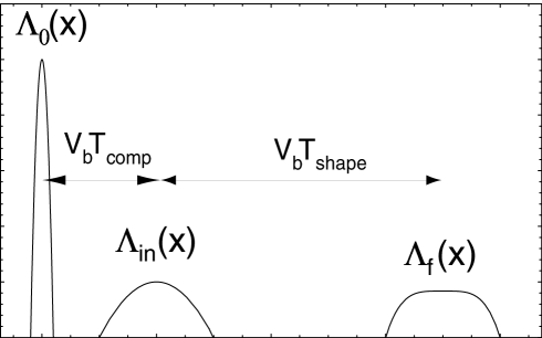
Figure 1:

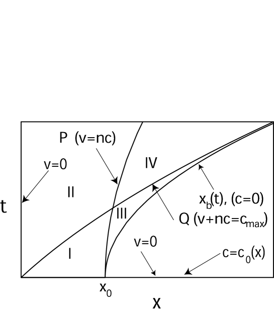
Figure 2:

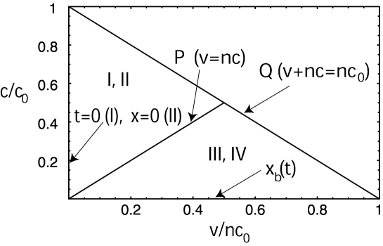
Figure 3:

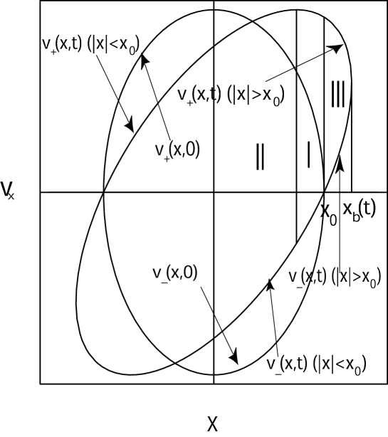
Figure 4:

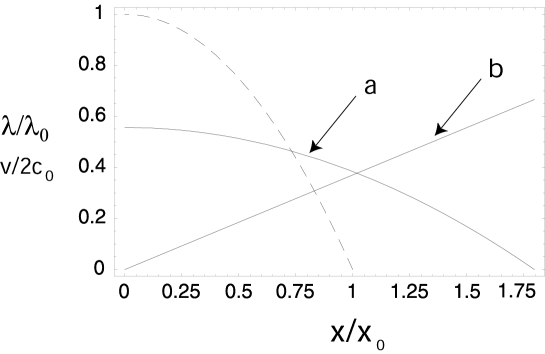
Figure 5:

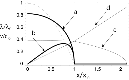
Figure 6:

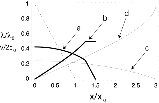
Figure 7:

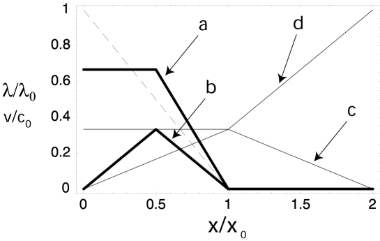
Figure 8:

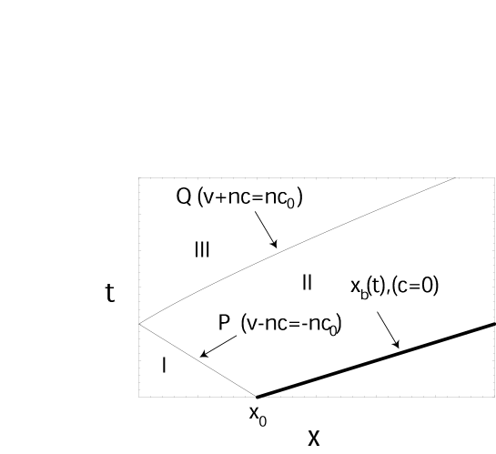
Figure 9:

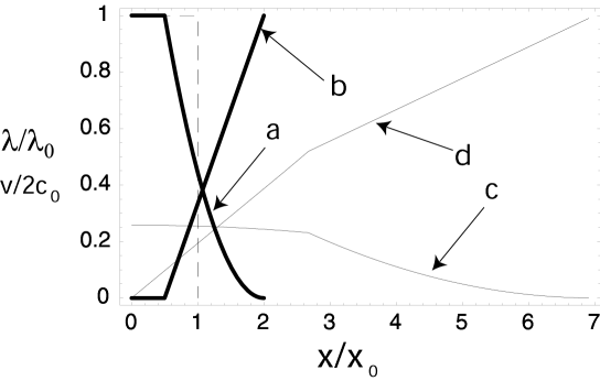
Figure 10:

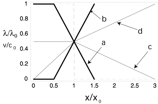
Figure 11:

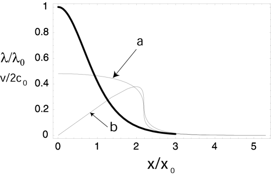
Figure 12:

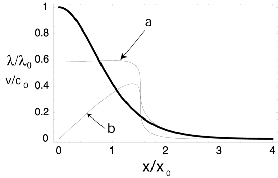
Figure 13:

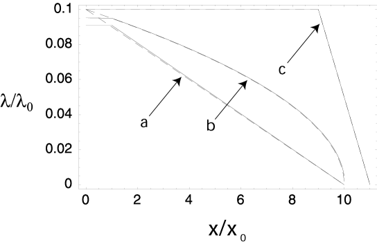
Figure 14:

Figure 15:

References

- (1) R. C. Davidson and H. Qin, Physics of Intense Charged Particle Beams in High Energy Accelerators (World Scientific, Singapore, 2001), and references therein.
- (2) M. Reiser, Theory and Design of Charged Particle Beams (Wiley, New York, 1994).
- (3) J. D. Lawson, The Physics of Charged-Particle Beams (Oxford Science Publications, New York, 1988).
- (4) A. W. Chao, Physics of Collective Beam Instabilities in High Energy Accelerators (Wiley, New York, 1993).
- (5) D. A. Edwards and M. J. Syphers, An Introduction to the Physics of High-Energy Accelerators (Wiley, New York, 1993).
- (6) I. M. Kapchinskij and V. V. Vladimirskij, in Proceedings of the International Conference on High Enegy Accelerators and Instrumentation (CERN Scientific Information Service, Geneva, 1959), p. 274.
- (7) R. L. Gluckstern, in Proceedings of the 1970 Proton Linear Accelerator Conference, Batavia, IL, edited by M. R. Tracy (National Accelerator Laboratory, Batavia, IL, 1971), p. 811.
- (8) T. -S. Wang and I. Smith, Part. Accel. 12, 247 (1982).
- (9) J. Hofmann, L. J. Laslett, L. Smith, and I. Haber, Part. Accel. 13, 145 (1983).
- (10) J. Struckmeier, J. Klabunde, and M. Reiser, Part. Accel. 15, 47 (1984).
- (11) I. Hofmann and J. Struckmeier, Part. Accel. 21, 69 (1987).
- (12) J. Struckmeier and I. Hofmann, Part. Accel. 39, 219 (1992).
- (13) N. Brown and M. Reiser, Phys. Plasmas 2, 965 (1995).
- (14) R. C. Davidson and H. Qin, Phys. Rev. ST Accel. Beams 2, 114401 (1999).
- (15) R. L. Gluckstern, W. -H. Cheng, and H. Ye, Phys. Rev. Lett. 75, 2835 (1995).
- (16) R. C. Davidson and C. Chen, Part. Accel. 59, 175 (1998).
- (17) C. Chen, R. Pakter, and R. C. Davidson, Phys. Rev. Lett. 79, 225 (1997).
- (18) C. Chen and R. C. Davidson, Phys. Rev. E 49, 5679 (1994).
- (19) R. C. Davidson, W. W. Lee, and P. Stoltz, Phys. Plasmas 5, 279 (1998).
- (20) R. C. Davidson, Phys. Rev. Lett. 81, 991 (1998).
- (21) R. C. Davidson, Phys. Plasmas 5, 3459 (1998).
- (22) P. Stoltz, R. C. Davidson, and W. W. Lee, Phys. Plasmas 6, 298 (1999).
- (23) W. W. Lee, Q. Qian, and R. C. Davidson, Phys. Lett. A 230, 347 (1997).
- (24) Q. Qian, W. W. Lee, and R. C. Davidson, Phys. Plasmas 4, 1915 (1997).
- (25) S. I. Tzenov and R. C. Davidson, Phys. Rev. ST Accel. Beams 5, 021001 (2002).
- (26) R. C. Davidson and H. Qin, Phys. Rev. ST Accel. Beams 4, 104401 (2001).
- (27) R. C. Davidson, H. Qin, and P. J. Channell, Phys. Rev. ST Accel. Beams 2, 074401 (1999); 3, 029901 (2000).
- (28) R. C. Davidson, A. Friedman, C. M. Celata, D. R. Welch, et al., Laser and Particle Beams 20, 377 (2002).
- (29) E. G. Harris, Phys. Rev. Lett. 2, 34 (1959).
- (30) E. A. Startsev, R. C. Davidson and H. Qin, Physics of Plasmas 9, 3138 (2002).
- (31) E. A. Startsev, R. C. Davidson and H. Qin, Laser and Particle Beams 20, 585 (2002).
- (32) E. A. Startsev, R. C. Davidson and H. Qin, Physical Review Special Topics on Accelerators and Beams 6, 084401 (2003).
- (33) E. A. Startsev and R. C. Davidson, Physical Review Special Topics on Accelerators and Beams 6, 044401 (2003).
- (34) R. A. Kishek, P. G. O’Shea, and M. Reiser, Phys. Rev. Lett. 85, 4514 (2000).
- (35) J. Haber, A. Friedman, D. P. Grote, S. M. Lund, and R. A. Kishek, Phys. Plasmas 6, 2254 (1999).
- (36) A. Friedman, D. P. Grote, and I. Haber, Phys. Fluids B 4, 2203 (1992).
- (37) E. S. Weibel, Phys. Rev. Lett. 2, 83 (1959).
- (38) E. A. Startsev and R. C. Davidson, Physics of Plasmas 10, 4829 (2003).
- (39) R. C. Davidson, D. A. Hammer, I. Haber and C. E. Wagner, Phys. Fluids 15, 317 (1972).
- (40) R. Lee and M. Lampe, Phys. Rev. Lett. 31, 1390 (1973).
- (41) C. A. Kapetanakos, Appl. Phys. Lett. 25, 484 (1974).
- (42) M. Honda, J. Meyer-ter-Vehn, A. Pukhov, Phys. Rev. Lett. 85, 2128 (2000).
- (43) V. K. Neil and A. M. Sessler, Rev. Sci. Instr. 36, 429 (1965).
- (44) E. P. Lee, in Proceedings of the 1981 Linear Accelerator Conference, Los Alamos National Laboratory Report LA-9234-C, pp. 263–265.
- (45) E. P. Lee, Particle Accelerators 37, 307 (1992).
- (46) R. C. Davidson, H. Qin and G. Shvets, Physical Review Special Topics on Accelerators and Beams 6, 104402 (2003).
- (47) D. Neuffer, B. Colton, D. Fitzgerald, T. Hardek, R. Hutson, R. Macek, M. Plum, H. Thiessen, and T. S. Wang, Nucl. Strum. Methods Phys. Res. A321, 1 (1992).
- (48) R. J. Macek, et al., Proceedings of the 2001 Particle Accelerator Conference 1, 688 (2001).
- (49) R. C. Davidson, H. Qin, and T. -S. Wang, Physics Letters A252, 213 (1999).
- (50) R. C. Davidson, H. Qin, P. H. Stoltz, and T. -S. Wang, Physical Review Special Topics on Accelerators and Beams 2, 054401 (1999).
- (51) R. C. Davidson and H. Qin, Physics Letters A270, 177 (2000).
- (52) H. Qin, R. C. Davidson and W. W. Lee, Physical Review Special Topics on Accelerators and Beams 3, 084401 (2000); 3, 109901 (2000).
- (53) R. C. Davidson and H. S. Uhm, Physics Letters A285, 88 (2001).
- (54) H. Qin, R. C. Davidson, E. A. Startsev and W. W. Lee, Laser and Particle Beams 21, 21 (2003).
- (55) T. -S. Wang, P. J. Channell, R. J. Macek, and R. C. Davidson, Physical Review Special Topics on Accelerators and Beams 6, 014204 (2003).
- (56) H. Qin, E. A. Startsev and R. C. Davidson, Physical Review Special Topics on Accelerators and Beams 6, 014401 (2003).
- (57) H. Qin, Physics of Plasmas 10, 2708 (2003).
- (58) E. P. Lee, Phys. Fluids 21, 1327 (1978).
- (59) E. J. Lauer, R. J. Briggs, T. J. Fesendon, R. E. Hester, and E. P. Lee, Phys. Fulids 21, 1344 (1978).
- (60) M. N. Rosenbluth, Phys. Fluids 3, 932 (1960).
- (61) H. S. Uhm and M. Lampe, Phys. Fluids 23, 1574 (1980).
- (62) H. S. Uhm and M. Lampe, Phys. Fluids 24, 1553 (1981).
- (63) R. F. Fernsler, S. P. Slinker, M. Lampe, and R. F. Hubbard, Phys. Plasmas 2, 4338 (1995), and references therein.
- (64) H. S. Uhm and R. C. Davidson, Physical Review Special Topics on Accelerators and Beams 6, 034204 (2003).
- (65) H. S. Uhm, R. C. Davidson and I. D. Kaganovich, Physics of Plasmas 8, 4637 (2001).
- (66) G. Joyce and M. Lampe, Phys. Fluids 26, 3377 (1983).
- (67) H. S. Uhm and R. C. Davidson, Phys. Fluids 23, 1586 (1980).
- (68) I. D. Kaganovich, G. Shvets, E. Startsev and R. C. Davidson, Physics of Plasmas 8, 4180 (2001).
- (69) I. Kaganovich, E. A. Startsev and R. C. Davidson, Laser and Particle Beams 20, 497 (2002).
- (70) D. V. Rose, P. F. Ottinger, D. R. Welch, B. V. Oliver and C. L. Olson, Phys. Plasmas 6, 4094 (1999).
- (71) D. R. Welch, D. V. Rose, B. V. Oliver, T. C. Genoni, C. L. Olson and S. S. Yu, Phys. Plasmas 9, 2344 (2002).
- (72) I. Hofmann, Z. Naturforsch. 37A, 939 (1982).
- (73) I. Hofmann, Laser and Particle Beams 3, 1 (1985).
- (74) O. Boine-Frankenheim, I. Hofmann and G. Rumolo, Phys. Rev. Lett. 82, 3256 (1999).
- (75) L. K. Spentzouris, J. -F. Ostiguy and P. L. Colestock, Phys. Rev. Lett. 76, 620 (1996).
- (76) L. K. Spentzouris, P. L. Colestock and C. Bhat, Proceedings of the 1999 Particle Accelerator Conference 1, 114 (1999).
- (77) R. Fedele, G. Miele, L. Palumbo and V. G. Vaccaro, Phys. Lett. A179, 407 (1993).
- (78) H. Schamel, Phys. Rev. Lett. 79, 2811 (1997).
- (79) H. Schamel and R. Fedele, Phys. Plasmas 7, 3421 (2000).
- (80) A. Hofmann, CERN Report No. 77-13 (1977).
- (81) D. Neuffer, Particle Accelerators, 11, 23, 1980.
- (82) C. K. Allen, N. Brown and M. Reiser, Particle Accelerators 45, 149 (1994).
- (83) W. M. Sharp, A. Friedman and D. P. Grote, Fusion Engineering and Design 32, 201 (1996).
- (84) J. G. Wang, H. Suk, D. X. Wang and M. Reiser, Phys. Rev. Lett. 72, 2029 (1994).
- (85) R. C. Davidson and E. A. Startsev, Physical Review Special Topics on Accelerators and Beams 7, 024401 (2004).
- (86) R. C. Davidson and S. Strasburg, Physics of Plasmas 7, 2657 (2000).
- (87) S. M. Lund and R. C. Davidson, Physics of Plasmas 5, 3028 (1998).
- (88) R. C. Davidson, H. Qin, S. I. Tzenov, and E. A. Startsev, Physical Review Special Topics on Accelerators and Beams 5, 084402 (2002).
- (89) L. D. Landau and E. M. Lifshitz, Fluid Mechanics, (Pergamon Press, Oxford, 1987).
- (90) H. Qin, R. C. Davidson, J. J. Barnard and E. P. Lee, in Proceedings of the 2003 Particle Accelerator Conference, 2658 (2003).
- (91) H. Qin and R. C. Davidson, Physical Review Special Topics on Accelerators and Beams 5, 03441 (2002).
- (92) H. Qin and R. C. Davidson, Laser and Particle Beams 20, 565 (2002).
- (93) I. Haber, in Proccedings of the Symposium on Accelerator Aspects of Heavy Ion Fusion, Darmstadt, 1982 (GSI, Darmstadt, 1982), p. 372.
- (94) I. Hofmann and I. Bozsik, in Proccedings of the Symposium on Accelerator Aspects of Heavy Ion Fusion, Darmstadt, 1982 (GSI, Darmstadt, 1982), p. 362.
- (95) J. Bisognano, E. P. Lee and J. W.-K. Mark, LLNL Report, No. 3-28, 1985.
- (96) D. D.-M. Ho, S. T. Brandon and E. P. Lee, Part. Accel. 35, 15 (1991).
- (97) M. J. L. de Hoon, PhD. thesis, University of California, Berkeley, 2001.
- (98) E. P. Lee and J. J. Barnard, in Proceedings of the 2001 Particle Accelerator Conference, Chicago, 2001, p. 2928.
- (99) H. Qin, C. Jun, R. C. Davidson and P. Heitzenroeder, in Proceedings of the 2001 Particle Accelerator Conference, Chicago, 2001, p. 1761
- (100) M. Abromowitz and I. Stegun, Handbook of Mathematical Functions, Dover, NY, 1972.