Orbit and Optics Improvement by Evaluating the Nonlinear BPM Response in CESR

Abstract

We present an improved system for orbit and betatron phase measurement utilizing nonlinear models of BPM pickup response. We first describe the calculation of the BPM pickup signals as nonlinear functions of beam position using Green’s reciprocity theorem with a two-dimensional formalism. We then describe the incorporation of these calculations in our beam position measurements by inverting the nonlinear functions, giving us beam position as a function of the pickup signals, and how this is also used to improve our measurement of the betatron phase advance. Measurements are presented comparing this system with the linearized pickup response used historically at CESR.

I Introduction

CESR measures beam position and betatron phase with approximately one hundred beam position monitors (BPMs) distributed around the storage ring. Each BPM consists of four button-type electrodes mounted flush with, and electrically isolated from, the surface of the beam pipe. A moving particle bunch induces charge on the beam pipe walls and on the surface of each button, which one can describe as image currents or as surface charge due to the transverse component of the bunch’s electric field Shafer (1992).

The BPM buttons are connected to electronics that process and record signals which are a function of the distance between the button and the passing bunch. The four signals from each BPM are used to determine the beam position and betatron phase advance. At many accelerators, the button signals’ nonlinear dependence on the beam position is linearized for simplicity. Before the improvements described here, this approach was also used in CESR.

Our efforts to improve the beam position measurements by including the nonlinear BPM response is motivated by CESR’s pretzel orbits, where electron and positron beams avoid parasitic collisions by following separate paths with large displacements from the central axis of the beam pipe. The linearized methods are not reliable for such large amplitudes, and have made accurate beam position and betatron phase measurements at CESR impossible under colliding beam conditions. We will illustrate those shortcomings and present measurements demonstrating improvement by using the nonlinear models.

II Background

\psfrag{S1}{$S_{1}$}\psfrag{S2}{$S_{2}$}\psfrag{S3}{$S_{3}$}\psfrag{S4}{$S_{4}$}\psfrag{x}{$x$}\psfrag{y}{$y$}\includegraphics[width=180.67499pt]{arc.eps}

Figure 1: Arrangement of buttons in CESR arc BPMs

Many accelerators, including CESR, have traditionally assumed a linear relationship between the beam position and the BPM button signals. Given four signals $S_{i}\>(i=1,\ldots,4)$ from buttons arranged as in Fig. 1, the transverse beam position is given approximately by

$$x = k_{x}\frac{(S_{2}+S_{4})-(S_{1}+S_{3})}{\Sigma_{i}S_{i}}$$ (1)

$$y = k_{y}\frac{(S_{3}+S_{4})-(S_{1}+S_{2})}{\Sigma_{i}S_{i}}$$ (2)

where $k_{x,y}$ are scale factors set by the geometry of each BPM type. This evaluation of BPM signals is often called the difference-over-sum method. Equations (1-2) provide an estimation of the bunch position in relatively few arithmetic operations.

Because analytical approaches to determining the factors $k_{x,y}$ make drastic approximations to the BPM geometry, we have tried to measure the factors experimentally at CESR through a variety of techniques summarized in Table 1. Those include translating a section of the beam pipe containing the BPM with precision actuators, using a test stand with a movable antenna to simulate the beam, and using the known value of the dispersion while changing the beam energy in dispersive regions Bagley and Rouse (1991).

Method	$k_{x}$ (mm)	$k_{y}$ (mm)
20 MHz antenna	25.58$\pm$.33	20.58$\pm$.43
Dispersion (1990)	26.3
Dispersion (1991)	27.4$\pm$.6
Moving beam pipe ($e^{+}$)	26.82$\pm$.25	19.96$\pm$.11
Moving beam pipe ($e^{-}$)	27.14$\pm$.54	20.48$\pm$.19
2D Poisson model	26.2	19.6

Table 1: Measured scale factors for CESR arc BPMs.

But precise knowledge of $k_{x,y}$ is of limited benefit, since Eqs. (1-2) yield only the linear part of the signal dependence for bunches near the center of the BPM. In the next section, we describe our technique for accurately calculating button signals, but let us first use those results to illustrate the limitation of the linearized formulae.

Figure 2: Linearized horizontal position measurement in an arc BPM. At a typical pretzel amplitude of 1.5 cm, the linearized formula shows significant disagreement with a linear fit.

In Fig. 2, the four button signals were calculated numerically for a beam at different horizontal displacements. The four signals were combined according to Eq. (1) and plotted against the known horizontal displacement. The slope near the origin gives $k_{x}^{-1}$, but the linear relationship breaks down noticeably at approximately 1 cm, and beyond 2 cm the relationship fails completely. Because pretzel orbits in CESR are typically as large as 1.5 cm, this is precisely what has hindered accurate measurements under colliding beam conditions until the improvements described in this paper were implemented.

Figure 3: Linearized map distortion in CESR interaction-point BPM with approximately circular cross-section.

Figure 4: Linearized map distortion in CESR arc BPM with approximately elliptical cross-section.

The problem of this nonlinearity is made even more evident in two dimensions. Figures 3-4 show a regular grid of $(x,y)$ points and the mapping of those same points under Eq. (1-2). Both BPMs show the characteristic pincushion distortion, which increases with distance from the origin.

In CESR, betatron phase measurements also rely on a related assumption about the linearity of the button signals. The betatron phase is measured by shaking the beam at a sideband of the betatron frequency. For each detector, the phase for each button is calculated by electronically comparing AC signal on that button to the phase of the shaking. From the individual horizontal (vertical) button phases $\theta_{h,i}\>(\theta_{v,i})$, the horizontal and vertical betatron phase is calculated by

$$A_{h}e^{i\theta_{h}} = e^{i\theta_{2,h}}+e^{i\theta_{4,h}}-e^{i\theta_{1,h}}-e^{i\theta_{3,h}}$$ (3)

$$A_{v}e^{i\theta_{v}} = e^{i\theta_{3,v}}+e^{i\theta_{4,v}}-e^{i\theta_{1,v}}-e^{i\theta_{2,v}},$$ (4)

where $A_{h,v}$ are real constants that are not used further Sagan et al. (2000). Other than the minus signs which account for the assumption that the beam is shaking between the pairs of buttons, this is simply an averaging of button phases represented as complex vectors.

When the horizontal orbit amplitude is large, the beam begins to shake underneath the buttons, and the relationship between the beam motion and the button signal becomes complicated. In such cases, some of the buttons may report an inaccurate phase, and averaging them with the rest corrupts the final answer. We will show how our nonlinear models can improve not only beam position measurements, but these measurements as well.

III An Improved System For Position And Phase Measurement

In order to overcome the limitations described, a new system has been implemented with two major components: realistic numerical models of the button response, and an efficient algorithm for inverting the model to yield beam position.

III.1 Numerical Calculation of BPM Response

For accurate beam position measurements, a function is required that expresses the bunch location $(x,y)$ as a nonlinear function of the button signals. Since the four button signals lead to two coordinates (and a scale factor), the problem is over-constrained, and this function cannot be obtained directly. The inverse (button signals from beam position), however, is readily obtainable by standard numerical techniques.

The most accurate and direct method of numerical solution is to simulate the bunch in a three-dimensional BPM, calculating the electromagnetic fields, and from them, the charge on the buttons. The simulation could be repeated for different beam locations, and the fields recalculated until enough solutions were accumulated to describe the behavior over the entire BPM. However, this is very computationally intensive, and can be avoided by the methods that follow.

III.1.1 Two-Dimensional Approximation

For ultra-relativistic bunches in a beam pipe with constant cross section, the approximate electromagnetic fields can be calculated using a two dimensional formalism Cupérus (1977); Krinsky (1989). Assuming the bunch has negligible transverse extent, the charge distribution of the bunch may be written, in the lab frame, as

$$\rho=\delta(\mathbf{r-r_{0}})\sum_{k}\rho_{k}\cos\left(k(z-vt)\right)$$ (5)

where the longitudinal dependence in $z$ has been written as a Fourier expansion. Transforming to the reference frame of the bunch, the charge density and electric potential are written

$$\rho^{*} = \delta(\mathbf{r-r_{0}})\sum_{k}\frac{\rho_{k}}{\gamma}\cos(kz^{*}/\gamma),$$ (6)

$$\Phi^{*} = \Phi(\mathbf{r})\sum_{k}\frac{\phi_{k}}{\gamma}\cos(kz^{*}/\gamma).$$ (7)

We write Poisson’s equation $\nabla^{2}\Phi^{*}=\rho^{*}$ in the bunch frame as

$$\left(\nabla^{2}_{\perp}-\frac{k^{2}}{\gamma^{2}}\right)\Phi(\mathbf{r})\phi_{k}=\delta(\mathbf{r-r_{0}})\rho_{k}$$ (8)

where $\nabla^{2}_{\perp}$ is the two-dimensional transverse Laplacian. For bunches with length $\sigma_{l}$ without appreciable longitudinal substructure, $\rho_{k}$ is only relevant for $k\leq\frac{1}{\sigma_{l}}$. The characteristic distance over which $\Phi(\mathbf{r})$ changes is the diameter $a$ of the beam-pipe so that the order of magnitude estimate $|\nabla^{2}_{\perp}\Phi(\mathbf{r})|\approx\frac{1}{a^{2}}|\Phi|$ can be made. For sufficiently long bunches and sufficiently large values of $\gamma$, the relevant values of $k/\gamma$ can be neglected, i.e. when $\frac{1}{\gamma^{2}}\ll(\frac{\sigma_{l}}{a})^{2}$ and the solution is described by the two dimensional, electrostatic case

$$\nabla^{2}_{\perp}\Phi(\mathbf{r})=\frac{\rho_{k}}{\phi_{k}}\delta(\mathbf{r-r_{0}}).$$ (9)

Since we only need $\Phi(\mathbf{r})$ up to a multiplicative factor, we don’t worry about the constant coefficients on the right-hand side.

III.1.2 Green’s Reciprocity Theorem

Rather than perform a separate calculation of the button signals for many beam positions, we use Green’s reciprocity theorem to calculate the button signals for all $(x,y)$ inside the BPM with a single numerical calculation. This theorem states that the surface charge $\sigma$ on a button due to a test charge at $(x,y)$ is proportional to the potential at that same position when the test charge is absent and the button is excited by a potential $\mathcal{V}$.

Suppose we have two scalar functions $\phi_{1}$ and $\phi_{2}$ in a volume $V$ bounded by a surface $S$. We form the vector field

$$\mathbf{A}=\phi_{1}\nabla\phi_{2}$$ (10)

for which the divergence theorem guarantees

$$\int_{V}\nabla\cdot\mathbf{A}\,dV=\oint_{S}\mathbf{A}\cdot\mathbf{\hat{n}}\,da.$$ (11)

Manipulating the integrands gives

$$\nabla\cdot(\phi_{1}\nabla\phi_{2}) = (\nabla\phi_{1})\cdot(\nabla\phi_{2})+\phi_{1}\nabla^{2}\phi_{2}$$ (12)

$$\mathbf{A}\cdot\mathbf{\hat{n}} = \phi_{1}\nabla\phi_{2}\cdot\mathbf{\hat{n}}=\phi_{1}\frac{\partial\phi_{2}}{\partial n}$$ (13)

where $\mathbf{\hat{n}}$ is a unit vector normal to the surface and pointing out of the volume of integration, and $\partial/\partial n$ indicates differentiation with respect that direction. Equation (11) yields

$$\int_{V}\left[(\nabla\phi_{1})\cdot(\nabla\phi_{2})+\phi_{1}\nabla^{2}\phi_{2}\right]\,dV=\oint_{S}\phi_{1}\frac{\partial\phi_{2}}{\partial n}\,da.$$ (14)

If we interchange $\phi_{1}$ and $\phi_{2}$ and subtract the result from Eq. (14), we can eliminate the first term in the integrand of the left hand side. This gives

$$\int_{V}\left[\phi_{1}\nabla^{2}\phi_{2}-\phi_{2}\nabla^{2}\phi_{1}\right]\,dV=\oint_{S}\left[\phi_{1}\frac{\partial\phi_{2}}{\partial n}-\phi_{2}\frac{\partial\phi_{1}}{\partial n}\right]\,da.$$ (15)

Taking the $\phi_{i}$ to be potentials for volume charge density $\rho_{i}$ and surface charge density $\sigma_{i}$ leads to Green’s reciprocity theorem:

$$\int_{V}\phi_{1}\rho_{2}\,dV+\oint_{S}\phi_{1}\sigma_{2}\,da=\int_{V}\phi_{2}\rho_{1}\,dV+\oint_{S}\phi_{2}\sigma_{1}\,da$$ (16)

where we have used $\nabla^{2}\phi=-\rho$ and $\partial\phi/\partial n=\sigma$ (recall that $\mathbf{\hat{n}}$ points into the conducting surface).

Connecting this result to the case of a BPM, imagine $\phi_{1}$ corresponds to the potential when a single button is excited with a potential $\mathcal{V}$ and all other surfaces are grounded. We can calculate the potential $\phi_{1}(x,y)$ by numerical solution of Laplace’s equation. For the second potential $\phi_{2}$, we ground all surfaces and put a charge distribution $\rho_{2}(x,y)$ inside the BPM.

We plug the two cases into Eq. (16) and observe that the third integral vanishes because there is no volume charge for the first case ($\rho_{1}=0$ in $V$). The fourth integral vanishes because we grounded the beam pipe and the buttons ($\phi_{2}=0$ on $S$). Since $\mathcal{V}$ can be pulled out of the second integral, what remains is just the total charge on the button, labeled $q_{b}$, giving

$$\int_{V}\phi_{1}(x,y)\rho_{2}(x,y)\,dV=-\mathcal{V}q_{b}.$$ (17)

If $\rho_{2}$ is a point charge $q$ located at $(x_{0},y_{0})$, then the integral in Eq. (17) picks out the value $\phi_{1}(x_{0},y_{0})$. We arrive at the final relation

$$q_{b}=-\frac{q\phi(x_{0},y_{0})}{\mathcal{V}},$$ (18)

remembering that $\phi(x,y)$ and $\mathcal{V}$ refer to the two different configurations.

Therefore, since the signal on a button is proportional to the induced surface charge on that button $q_{b}$, $\phi(x_{0},y_{0})$ is the solution to the problem of calculating the button signal, up to a multiplicative constant, as a function of the bunch location.

III.1.3 Calculation of the Button Signals

Based on the previous arguments, we use POISSON to solve the boundary value problem for $\phi(x,y)$. For the two-dimensional boundary, we take a slice at the longitudinal midplane of each BPM. The first button is set (arbitrarily) at 10 volts and all other surfaces are grounded. POISSON generates a mesh inside the boundary, computes the solution to Laplace’s equation on the mesh, and stores the result at regular grid points in an output file.

CESR BPMs have multiple geometric symmetries, so the signals $\phi_{i}(x,y)$ on the other three buttons are just reflections or rotations of the coordinates for the excited button in the first calculation of $\phi_{1}(x,y)$. To compute $\phi_{i}(x,y)$ between grid points, we use bicubic interpolating polynomials, which are stored for quick subsequent evaluation.

III.2 Realtime Inversion

For beam position measurements, we start with button signals $S_{i}$ and seek the location $(x,y)$ of the beam. The result $\phi_{i}(x,y)$ from the POISSON calculation must be inverted, and since we have four constraints (four buttons) and three parameters (position $(x,y)$, and a scale factor) we proceed by fitting the calculated button signals to the measured signals. We minimize the merit function

$$\chi^{2}=\sum_{i=1}^{4}\frac{\left(q\phi_{i}(x,y)-S_{i}\right)^{2}}{\sigma_{i}^{2}},$$ (19)

where $\phi_{i}(x,y)$ is the signal on the $i^{\mathrm{th}}$ button and the $\sigma_{i}$ are the uncertainties in the measured signals (which we take to be the same for all four buttons). The factor $q$ is proportional to the beam current and could be used for beam loss studies.

Minimization is performed via the Levenberg-Marquardt method provided in Numerical Recipes. This requires an initial guess for the parameters, which we find by scanning only the grid points of $\phi(x,y)$ (without evaluating the interpolating polynomials) for the values of the parameters that minimize $\chi^{2}$. Then we iteratively minimize over the continuous functions, typically arriving within less than $10^{-6}$ m of the minimum after six steps.

III.3 Phase Measurements

We can improve our measurement of the betatron phase advance between BPMs by incorporating our knowledge of the nonlinear button response. In this measurement, the beam is excited to small oscillations around its equilibrium position $(x_{0},y_{0})$. Let the phase and amplitude of the AC signal on the $i^{\mathrm{th}}$ button be represented by the complex number $\mathbf{C}_{i}$, and let the phase and amplitude of the horizontal and vertical components of the oscillatory beam motion be represented by complex numbers $\mathbf{A}_{x}$ and $\mathbf{A}_{y}$, respectively. To first order, their relationship is given by

$$\mathbf{C}_{i}=r_{i,x}\mathbf{A}_{x}+r_{i,y}\mathbf{A}_{y},$$ (20)

where the $r_{i,(x,y)}$ are given by

$$r_{i,x} = \left.q\frac{d\phi_{i}(x,y)}{dx}\right|_{(x_{0},y_{0})}$$ (21)

$$r_{i,y} = \left.q\frac{d\phi_{i}(x,y)}{dy}\right|_{(x_{0},y_{0})}.$$ (22)

The $\phi_{i}$ are the functions described in the previous section. Their derivatives are easily calculated from the coefficients of their interpolating polynomials.

Given the measured $\mathbf{C}_{i}$, we calculate $\mathbf{A}_{x}$ and $\mathbf{A}_{y}$ by minimizing

$$\chi^{2}=\sum_{i=1}^{4}\frac{1}{\sigma_{i}^{2}}|r_{i,x}\mathbf{A}_{x}+r_{i,y}\mathbf{A}_{y}-\mathbf{C}_{i}|^{2}.$$ (23)

Since the $\sigma_{i}$ depend on the closed orbit deviation and the values of $\mathbf{A}_{x,y}$, the minimization must also be performed iteratively. The horizontal and vertical phase advance is then given by the complex phase of $\mathbf{A}_{x}$ and $\mathbf{A}_{y}$. Whenever a horizontal excitation creates a vertical amplitude, or vice versa, this method is used in CESR to compute the coupling coefficients also.

IV Results

Testing the new system presents a challenge in that we can only produce controlled large amplitude orbits with the electrostatic separators. Since the separators are calibrated from BPM measurements, they do not provide an independent check on our ability to measure large amplitudes accurately. Our strategy, therefore, must be to use other measurements to check the accuracy at small amplitudes, and then confirm the expected linear relation between the separator strength and the beam position at large amplitudes.

Figure 5: Beam position at various detectors showing little or no bunch length dependence.

To perform a two-dimensional approximation, we argued that the bunches are sufficiently long. To verify that assumption, we have looked experimentally for a bunch length dependence in large amplitude orbits. With the pretzel at its nominal value of about 1.5 cm closed orbit deviation, the bunch length was calculated from the measured synchrotron tune, which we adjust by changing the RF accelerating voltage. As Fig. 5 illustrates, the beam position shows little or no dependence over the range of bunch lengths we expect in CESR.

Figure 6: Measured and calculated dispersion.

Changing the RF frequency in CESR changes the beam energy, and in dispersive regions, changes the beam position by up to a few millimeters. Measuring the beam position at many different energies allows us to measure the dispersion, which we compare to the theoretical value from the lattice in Fig. 6. This agreement verifies the small amplitude, or linear part of our nonlinear models.

Figure 7: Beam position at two detectors calculated with the nonlinear and linearized methods.

To observe the large amplitude accuracy of the new system, we rely on the electrostatic separators to change the orbit amplitude linearly. By increasing the horizontal separator strength, we observe in Fig. 7 that the orbit calculated with the nonlinear method does show the correct behavior, while the orbit calculated with the linearized formula shows the deviation that was illustrated in Fog. 2.

Figure 8: Separator scan. Orbits at detector 9W calculated using linearized (dashed) and nonlinear (solid) methods.

To demonstrate improvement in two dimensions, the voltages on individual horizontal and vertical separators were scanned over a regular grid. The measured beam positions should also lie on a regular grid, which is shown in Fig. 8. Some sheering is evident in the plot, which may be due to coupling of the vertical and horizontal motion between the separator and the BPM, or to a rotation of the BPM. The pincushion effect is notably reduced with the new calculation.

Figure 9: Difference in horizontal betatron phase advance between data and model with large closed orbit distortion after using a phase correction algorithm based on the linear (dashed) and nonlinear (solid) BPM evaluation.

We use betatron phase measurements to correct the difference between the physical optics and the values in our model lattice. Without the nonlinear correction, large closed orbit distortions hindered this process since the data we sought to fit did not correspond to the actual phase. Figure 9 shows the drastically improved agreement we can achieve between the model phase and the data when the new BPM calibration is used.

V BPM Calibration

The response of a particular BPM may differ from that of the computational model (linear or nonlinear) for a variety of reasons. The leading candidate for this effect is the variation in insertion depth of the individual buttons (i.e., the distance from the button surface to the surface of its cylindrical housing). This manifests itself as different gains for the signals from different buttons.

Following the method of Lambertson (1987); Keil (2000), we determine the gain for each button from the capacitive coupling between each pair of buttons. If the ideal coupling between two buttons is given by $U_{ij}$, then the measured coupling will be $\tilde{U}_{ij}=b_{i}b_{j}U_{ij}$ where $b_{i},b_{j}$ are the effective gains of the input and output button, respectively. Symmetric pairs of buttons have equal ideal coupling, so $U_{12}=U_{34}$, $U_{13}=U_{24}$, and $U_{14}=U_{23}$.

Using this symmetry for the six measurements $\tilde{U}_{ij}\>(i=1,\ldots,3,\>j=i+1,\ldots,4)$ we can calculate the four $b_{i}$ up to an multiplicative factor. Normalizing to $b_{1}$ gives

$$b_{1} = 1\ ,$$ (24)

$$b_{2} = \sqrt{\frac{\tilde{U}_{23}\tilde{U}_{24}}{\tilde{U}_{13}\tilde{U}_{14}}}\ ,$$ (25)

$$b_{3} = \sqrt{\frac{\tilde{U}_{23}\tilde{U}_{43}}{\tilde{U}_{12}\tilde{U}_{14}}}\ ,$$ (26)

$$b_{4} = \sqrt{\frac{\tilde{U}_{24}\tilde{U}_{43}}{\tilde{U}_{12}\tilde{U}_{13}}}\ .$$ (27)

These gain coefficients are used to correct the button signals before calculating the beam position.

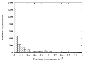
Figure 10: Fractional improvement in the $\chi^{2}$ of the beam position fit due to the calibration coefficients ($-1=100\%$ improvement).

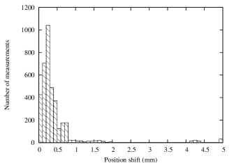
Figure 11: Correction in the calculated position due to the calibration coefficients.

With data drawn from approximately 3700 individual beam position measurements, Fig. 10 shows that when these coefficients are employed, the $\chi^{2}$ of the fit between the measured signals and the modeled signals is significantly reduced. The resulting correction to the calculated position is shown in Fig. 11 to be approximately 0.5 mm.

VI Conclusion

Two-dimensional, electrostatic models of BPM pickup response have been used with great success at CESR to measure beam position and betatron phase advance for large closed orbit distortions.

Calibration of our BPMs has reduced measurement errors due to button misalignments.

VII Acknowledgments

The authors wish to thank REU student Beau Meredith for his calibration of most of CESR’s BPMs.

References

- Shafer (1992) R. E. Shafer, in Physics of Particle Accelerators, edited by M. Month and M. Dienes (American Institute of Physics, New York, 1992).
- Bagley and Rouse (1991) P. Bagley and G. Rouse, CBN 17 (1991).
- Sagan et al. (2000) D. Sagan, R. Meller, R. Littauer, and D. Rubin, Physical Review Special Topics - Accelerators and Beams 3 (2000).
- Krinsky (1989) S. Krinsky, in Frontiers of Particle Beams; Observation, Diagnosis, and Correction, edited by M. Month and S. Turner (Springer-Verlag, Berlin, 1989).
- Cupérus (1977) J. Cupérus, Nuclear Instruments and Methods 145, 219 (1977).
- Lambertson (1987) G. Lambertson, LSAP Note-5 (1987).
- Keil (2000) J. Keil, Ph.D. thesis, Universität Bonn (2000).