A Variational Procedure for Time-Dependent Processes

Abstract

A simple variational Lagrangian is proposed for the time development of an arbitrary density matrix, employing the ”factorization” of the density. Only the ”kinetic energy” appears in the Lagrangian. The formalism applies to pure and mixed state cases, the Navier-Stokes equations of hydrodynamics, transport theory, etc. It recaptures the Least Dissipation Function condition of Rayleigh-Onsager and in practical applications is flexible. The variational proposal is tested on a two level system interacting that is subject, in one instance, to an interaction with a single oscillator and, in another, that evolves in a dissipative mode.

1 Introduction

Several basic aspects of stochastic dynamics remain controversial. (A critical ”state of art” update in [1] shows this). This situation contrasts with most physical theories, where the problems that arise are in the application of consensually accepted principles. It can perhaps be argued, that the lack of an agreed-upon variational formulation of stochastic processes is at the root of the problem. As a remedy of this situation, this article suggests a new variational functional which is to be minimized and whose minimum is the true density matrix.

To be sure, in the past several principles of extrema have been proposed; these include Gauss’s Least Constraint Principle [2, 3], the ”least dissipation function” [4, 5, 6], minimum entropy production-rate for steady states [7, 8] (see also [9] for its violation), minimal energy generation rate [10], minimal scattering integral ([11] - [13]), least velocity error during pathway [3], the Yasue Action for stochastic mechanics [14], a formulation involving a potential [15], and again, recently, maximum entropy production [16]. To these may be added several variational methods applicable to classical (i.e., not quantal) systems, such as those appropriate for general non-linear problems [17], the ”governing principle for Dissipative Processes” [18, 19] and a generalized Hamiltonian principle [20]. Reviews of these and of other methods can be found in [21] - [24].

The present proposal for a variational procedure is based on the following new elements: (a) the factorization (to be discussed later in this paper) of the density matrix as introduced by Reznik [25] and utilized recently by Gheorghiu-Svirschevski [16], (b) a conventional Lagrangian similar to that used in Mechanics to obtain the motion of a point particle subject to an external force, but in which the scalar potential is either absent or ignorable, (c) a vector potential that can be singular, without this having disastrous observational consequences and (d) an appropriate use of minimization procedure, with origins going back to Gibbs [2]. The method covers a broad range of behaviors (”deterministic” and stochastic, quantal and classical, electronic transport, discrete and continuous, markovian and otherwise) and places in a new perspective certain aspects in currently employed theories of stochastic dynamics. Apart from these favorable (and a priori unexpected) features, a number of problems remain, which will have to be resolved by future efforts.

A pure state sub-case, (as opposed to a density matrix that can describe a statistical mixture of states) is the subject of a numerically worked out example in section 4.1 and is equivalent to the (linear) time dependent Schrödinger equation. For this several variational formulations are known in the literature ([26] -[31]). The inter-relation between these was investigated in [30], where they were shown to be frequently equivalent. For the pure state case our density matrix variational method reduces to the McLachlan formalism [27], in which the variation of the function is carried out with respect to the time-derivative only (while the function is kept fixed). Moreover, we give a justification of this procedure for stochastic processes.

Another application of the variational formalism, in section 4.2, includes a non-linear, dissipative (non-Hermitian) mechanism and exemplifies quantum jumps.

2 The Variation

The ”factorized” form of the time dependent density matrix $\rho$ ([25],[16]) reads in terms of the column and row vectors ${{\bf\gamma}}$ and (its hermitian conjugate) ${\bf\gamma^{+}}$

$${\bf\rho={\bf\gamma}{\bf\gamma^{+}}}$$ (1)

The above condensed notation is not trivially simple, so we give in Appendix A a ”tutorial” on the notation. We now propose an action $S(T)$ (expressed in arbitrary units) this being the integral over time $t$ with an arbitrary time end-point $T$ of a Lagrangian $\cal L$. It is the form of the Lagrangian that we seek: we propose that it has the ”quadratic” form, as follows.

$$S(T) = \int_{0}^{T}dt\ {\cal L}(t)$$ (2)

$$= \int_{0}^{T}dt\ Tr\ (i{\dot{\gamma}^{+}}-{\bf A}^{+})\cdot(-i{\dot{\gamma}}-{\bf A})$$

The variational equations based on the above action (these are the equations of motions for ${{\bf\gamma}}$ and ${\bf\gamma^{+}}$) are given below in equation (7) . Tr is the trace over all ”components” of ${\bf\gamma}$ explained in Appendix A. Dots above symbols represent differentiation with time.

The variational equations are obtained in the usual way by varying the action $S(T)$ with respect to all components of the two vectors ${\bf\gamma}$ and ${\bf\gamma^{+}}$. Thus

$$\\ {\delta_{{\bf\gamma}}}S(T)=\int_{0}^{T}dt\delta{\bf\gamma}(t)[\frac{\delta{\cal L}(t)}{\delta{\bf\gamma}}-\frac{\partial}{\partial t}\frac{\delta{\cal L}(t)}{\delta\dot{\bf\gamma}}]+\frac{\delta{\cal L}(T)}{\delta\dot{\bf\gamma}}{\delta{\bf\gamma}}(T)$$ (3)

and a similar expression for ${\delta_{{\bf\gamma^{+}}}}S(T)$. The last term, outside the integral, is the boundary term. It is assumed that the vectors ${\bf\gamma}$ are fixed initially at $t=0$, but not at any time later. (This will be discussed shortly.) If the boundary term can be made to vanish, then so will be the whole variation, since in the absence of a scalar potential, the variations $\frac{\delta{\cal L}(t)}{\delta{\bf\gamma}}$ and $\frac{\delta{\cal L}(t)}{\delta{\gamma^{+}}}$ vanish. This follows, since for the postulated form of the Lagrangian these variations contain as a factor one or the other of the expressions $\frac{\delta{\cal L}(t)}{\delta\dot{\bf\gamma}}$ and $\frac{\delta{\cal L}(t)}{\delta{\dot{\gamma}^{+}}}$ and these vanish due to the boundary variation. (In fact, $\frac{\delta{\cal L}(t)}{\delta{\bf\gamma}}$ and $\frac{\delta{\cal L}(t)}{\delta{\gamma^{+}}}$ also vanish due to the presence of the same factors, but these variations do not form a sufficiently general basis for the variation procedure, since the vector potential $\bf A$ may not be a function of all components of the $\gamma$-vector.)

At this point the role of the boundary term is well worth reflecting upon. It is not present in, e.g., deterministic Mechanics, where the values of the variables are fixed at both end points. However, it is well known that the boundary term arises when the value of the variant quantity, i.e. ${\bf\gamma}$, is undetermined at a boundary. This is (physically) the case when a random force operates on the system. Thus, we are not allowed to neglect the boundary term. It is now a further ”bonus” in the formalism, that the vanishing of the boundary-term variation does not interfere with the vanishing of the body terms-variation, (i.e., it is neither contradictory to it nor incomplete with respect to it), but is by virtue of our choice of the Lagrangian precisely identical with it.

In summary, we have the variational equations

$$\frac{\delta{\cal L}(t)}{\delta\dot{\bf\gamma}}=0$$ (4)

and their complex conjugates

$$\frac{\delta{\cal L}(t)}{\delta{\dot{\gamma}^{+}}}=0$$ (5)

and these make the action extremal (and an absolute minimum) also when the ”vector potential” $\bf A$ is a function of ${\bf\gamma}$ [32].[To see this, note the remark after equation (7) ] This has the immediate consequence that in the expansion of the Lagrangian, shown in equation (2) , the following expression needs to be minimized:

$${}^{\prime}DF^{\prime}={\dot{\gamma}^{+}}{\dot{\gamma}}-i[{\dot{\gamma}^{+}}{\bf A}-{\dot{\gamma}}{\bf A^{+}}]$$ (6)

This follows, since the ${\bf A\cdot A^{+}}$ term is independent of time-derivatives and is not varied. We further note that (by the form of the vector potential) $i$ times the square bracket is a real quantity. The quantity in the above equation is essentially of the form of Onsager and Machlup’s Dissipation Function [the negative of eq. (4-25) in [5]. One recalls that their Dissipation Function is also minimized only with respect to the time derivatives of the variables just as in the procedure proposed in [27] and in the present work]. To bring our ’DF’ precisely to the form of the Dissipation Function, we need to go from our variables ${\bf\gamma}$ and ${\bf\gamma^{+}}$ by a constant linear transformation (not necessarily a unitary one) to the variables ${\bf\alpha}$ of [5]. One will then get, instead of the diagonal form ${\dot{\gamma}^{+}}{\dot{\gamma}}$, a non-diagonal form which defines the ”generalized resistance matrix” $R_{ij}$ of [3, 6]. [Since the use of extensive variables is to be preferred to intensive ones (and ${\bf\gamma}$ and ${\bf\gamma^{+}}$ are of the latter type) the transformation should include the system size. Alternatively, the action integral may be premultiplied by a size-dependent scale factor.]

Thus, the result of the variation are a set of equations:

$${\dot{\gamma}} = i{\bf A}$$

$${\dot{\gamma}^{+}} = -i{\bf A^{+}}$$ (7)

When $\bf A$ and $\bf A^{+}$ are functions of $\gamma$ and ${\gamma^{+}}$, their (non-zero) derivatives come in with either ${\dot{\gamma}}-i{\bf A}$ or ${\dot{\gamma}^{+}}+i{\bf A^{+}}$ as factors and these factors vanish due to the above equations.

[We can illustrate this in the case of two components, for which we write the Lagrangian in equation (1) as

$${\cal L}(t)=f_{1}^{+}f_{1}+f_{2}^{+}f_{2}$$ (8)

and $f_{1}=-i{\dot{\gamma}}_{1}-{\bf A}_{1}(\gamma_{k},\gamma_{k}^{+})$ etc. with the $\gamma$ dependence explicitly put in the $A$’s. Recall that equation (7) means that for the variational solution $f_{1}=f_{1}^{+}=f_{2}=f_{2}^{+}=0$ at all times and that with this solution the minimal action is zero.

Upon varying with respect to e.g., $\gamma_{1}$, the resulting Lagrange-Euler equations is now in full detail

$$-(\partial_{\gamma_{1}}A_{1}^{+})f_{1}+i{\dot{f}}_{1}^{+}-f_{1}^{+}(\partial_{\gamma_{1}}A_{1})-(\partial_{\gamma_{1}}A_{2}^{+})f_{2}-f_{2}^{+}(\partial_{\gamma_{1}}A_{2})=0$$ (9)

Since all the terms contain one of the $f$-factors or their time derivatives (which are necessarily also zero) the above equation is satisfied for the proposed variational solution. There may be other solutions, though! If for these not all $f$-s are zero (and therefore differ from the proposed solution), than the action (which consists of positive terms) is positive and larger than that for the solution given in equation (7) .]

These are the equations of motion of the (independent) vector variables and can be regarded as having the status of the Langevin equations, or Hamilton’s equations for the set of conjugate variables $\gamma_{a}$ and $\gamma^{+}_{a}$. The processes considered in this section comprise a purely Hamiltonian process $A_{H}$ (namely, energy preserving, ”elastic”) as well as some other, dissipative mechanisms. Thus, a Markovian scattering process represented by the symbol $M_{ba}$ (designating half the probability per unit time of a scattering event taking the system from state $a$ to $b$) can be written as $(A_{out},A_{in})$ to separate scattering out of and into a given state. We also add a stochastic, random process arising from, e.g., an external source, as $A_{r}$. Some other type of processes will be considered below in section 5.

For the first two processes we have

$$A_{H} = -H\gamma$$

$$A_{H}^{+} = -\gamma^{+}H^{+}=-\gamma^{+}H$$

$$(A_{out})_{a} = i\sum_{b}M_{ba}\gamma_{a}$$

$$(A_{out}^{+})_{a} = -i\gamma_{a}^{+}\sum_{b}M_{ba}$$

$$(A_{in})_{a} = -i\frac{1}{N}(\sum_{b}M_{ab}\gamma_{b}\gamma^{+}_{b})(\gamma_{a}^{+})^{-1}$$

$$(A_{in}^{+})_{a} = i(\gamma_{a})^{-1}(\frac{1}{N}\sum_{b}M_{ab}\gamma_{b}\gamma^{+}_{b})$$ (10)

When we add to these the random force, we obtain in addition

$$(A_{r})_{a}=-if_{a}\gamma_{a}\qquad(A_{r}^{+})_{a}=i\gamma_{a}f_{a}$$ (11)

$f_{a}$ represent the components of the random time-dependent force with zero mean and a finite self-correlation. ($N$ is the number of states in the ensemble, see appendix A)

The vector potential $\bf A_{in}$ is singular. However, singularities in vector potentials are well known (as, e.g., in those for solenoidal or monopole fields). To cancel these singularities we shall follow the procedure of Reznik [25] and Gheorghiu-Svirshevski [16], who multiply ${\bf\gamma^{+}}$ into ${\dot{\gamma}}$, ${\bf\gamma}$ into ${\dot{\gamma}^{+}}$, add and obtain the (master) equations for the density matrix.

After substituting the quantities from equations (7,10,11) we obtain by this procedure for a diagonal element (say) $aa$ of the density matrix

$$\dot{\rho}_{aa}=({\dot{\gamma}}{\bf\gamma^{+}}+{\bf\gamma}{\dot{\gamma}^{+}})_{aa}=i([\rho,H])_{aa}-2\rho_{aa}\sum_{b}M_{ba}+2\sum_{b}M_{ab}\rho_{bb}+2\rho_{aa}f_{a}$$ (12)

When one writes out the equation, similar to equation (12) , for the time derivatives of the off-diagonal matrix elements $\rho_{ab}(a\neq b)$, one finds singularities in them, due to the above mentioned singularities in the vector potentials. For a macroscopic system these singularities cancel, when one takes into account the phase decoherence between different states of macroscopic bodies. (The subject of microscopic to macroscopic transitions does not belong here. It was studied by various methods and has summaries in e.g. [33, 34].)

3 Potential Fluid Dynamics

An interesting application of the preceding complex factor-density formalism is for the well known potential flow (namely, fluid dynamics without vorticity) as presented in many hydrodynamic text books, e.g., [35]. If a flow satisfies the condition of zero vorticity, i.e. the velocity field $\vec{v}$ is such that $\vec{\nabla}\times\vec{v}=0$, then there exists a function $\phi$ satisfying $\vec{v}=\vec{\nabla}\phi$.

In this section we answer the question: what form of the vector potential ${\bf A}$ appearing in equation (2) will ensure, that upon variation of the action containing these vector potentials we shall obtain precisely the well known equations of potential flow hydrodynamics. These equations are:

$$\frac{\partial\rho}{\partial t} + \vec{\nabla}\cdot(\rho\vec{\nabla}\phi)=0$$ (13)

$$\frac{\partial\phi}{\partial t} = -\frac{1}{2}(\vec{\nabla}\phi)^{2}-h-\Phi-\nu\nabla^{2}\phi$$ (14)

In these equations the physical meaning of the quantities is that $\rho$ is the mass density, $h$ is the specific enthalpy, $\nu$ is the viscosity coefficient and $\Phi$ is some function representing the potential of an external force acting on the fluid. The first of these equations is the continuity equation, while the second is a modified Bernoulli’s equation which takes into account some viscous effects (A full viscous flow is of course not a potential flow and contains vorticity) . $\rho$ and $\phi$ play the roles of the squared-amplitude and of the phase angle, respectively. Both are real quantities.

The final results for the desired vector potentials and their complex conjugates are shown, below, in equation (23) and equation (24) . To obtain them, we first express the variational variables $\gamma$ and $\gamma^{+}$ that we have used so far in terms of the physical variables $(\rho,\phi)$. The variation will now be carried out with respect to the latter variables. The transformation is

$$\gamma = \sqrt{\rho}e^{i\phi}$$ (15)

$$\gamma^{+} = \sqrt{\rho}e^{-i\phi}$$ (16)

Though all variables are now functions of the positions, and are thus continuous variables, we shall label them, as before, by the subscripts $a$, etc. The following relations (with no summations over repeated symbols) arise simply from the inverse transformation:

$$\dot{\phi}_{a} = ({\dot{\gamma}}_{a}{\gamma^{+}}_{a}-\gamma_{a}{\dot{\gamma}^{+}}_{a})/2i\rho_{aa}$$ (17)

$$\vec{\nabla}\phi_{a} = (\vec{\nabla}\gamma_{a}{\gamma^{+}}_{a}-\gamma_{a}\vec{\nabla}{\gamma^{+}}_{a})/2i\rho_{aa}$$ (18)

$$\nabla^{2}\phi_{a} = (\nabla^{2}\gamma_{a}{\gamma^{+}}_{a}-\gamma_{a}\nabla^{2}{\gamma^{+}}_{a})/2i\rho_{aa}$$ (19)

$$-((\vec{\nabla}\gamma_{a}{\gamma^{+}}_{a})^{2}-(\gamma_{a}\vec{\nabla}{\gamma^{+}}_{a})^{2})/2i\rho_{aa}^{2}$$

$$\vec{\nabla}\rho_{aa} = (\vec{\nabla}\gamma_{a}{\gamma^{+}}_{a}+\gamma_{a}\vec{\nabla}{\gamma^{+}}_{a})$$ (20)

Using these, we first rewrite equation (13) as

$$\dot{\rho}_{aa} = ({\dot{\gamma}}_{a}{\gamma^{+}}_{a}+\gamma_{a}{\dot{\gamma}^{+}}_{a})=-\rho_{aa}\nabla^{2}\phi_{a}-\vec{\nabla}\rho_{aa}\cdot\vec{\nabla}\phi_{a}$$ (21)

$$\equiv R_{a}(\gamma_{a},{\gamma^{+}}_{a})$$

$R_{a}$ being a well-defined, real function of the variational variables and of their first and second spatial derivatives (but independent of the time-derivatives). Likewise, one obtains as the rate equation for the phase, equation (14) , as

$$\dot{\phi}_{a} = -({\dot{\gamma}}_{a}{\gamma^{+}}_{a}-\gamma_{a}{\dot{\gamma}^{+}}_{a})/2i\rho_{aa}$$ (22)

$$= -\frac{1}{2}(\vec{\nabla}\phi)^{2}-h-\Phi-\nu\nabla^{2}\phi$$

$$\equiv N_{a}(\gamma_{a},{\gamma^{+}}_{a})$$

in which $N_{a}$ has properties similar to $R_{a}$.

We can solve for the two quantities, ${\dot{\gamma}}_{a}{\gamma^{+}}_{a}$ and $\gamma_{a}{\dot{\gamma}^{+}}_{a}$ from the preceding two equations, and then divide by ${\gamma^{+}}_{a}$ and $\gamma_{a}$, respectively, to obtain the time derivatives. However, by equation (2) the time derivatives are just the vector potentials. Thus we finally obtain

$${\dot{\gamma}}_{a}=(R_{a}+2i\rho_{aa}N_{a})\frac{1}{2{\gamma^{+}}_{a}}=iA_{a}$$ (23)

and the complex conjugates

$${\dot{\gamma}^{+}}_{a}=\frac{1}{2\gamma_{a}}(R_{a}-2i\rho_{aa}N_{a})=-iA_{a}^{+}$$ (24)

We have thus found the vector potentials which have to be inserted in the action, so as to yield variationally the hydrodynamic equations, equation (13) and equation (14) . It is evident that the complex representation is a natural way to obtain variationally equations of motion for two such dissimilar quantities as amplitude and velocity. The physical extrema are certainly global minima (although the functional may have additional minima). Detailed applications will be undertaken in the future including the problem of a general viscous flow.

4 Applications

4.1 A Periodically Varying Hamiltonian

We shall now apply the proposed variational procedure to yield, in one case exactly and in another case approximately, the solution for a (hermitian) Hamiltonian that has a periodic variation. The cases chosen are such that analytical solutions are known exactly ([37]-[39]), so that we can compare to them the variational solutions to be obtained here. Specifically, we consider the time development of a doublet subject to a Schrödinger equation whose Hamiltonian in a doublet representation is

$$H(t)=G/2\left(\begin{array}[]{cc}-cos(\omega t)&sin(\omega t)\\ sin(\omega t)&cos(\omega t)\end{array}\right)$$ (25)

Here $\omega$ is the angular frequency of an external disturbance. The eigenvalues of equation (25) are $\frac{G}{2}$ and $-\frac{G}{2}$. If $G>0$, then in the ground state the amplitude in the upper component $\left(\begin{array}[]{c}1\\ 0\end{array}\right)$ in equation (25) is

$$C^{u}_{g} = \cos(Kt)\cos(\omega t/2)+(\omega/2K)\sin(Kt)\sin(\omega t/2)$$ (26)

$$+ i(G/2K)\sin(Kt)\cos(\omega t/2)$$

with

$$K=0.5\sqrt{G^{2}+\omega^{2}}$$ (27)

The amplitude $C^{l}_{g}$ of lower component $\left(\begin{array}[]{c}0\\ 1\end{array}\right)$ in the ground state has a similar form, which we shall not bother to write out. For the variational procedure we postulate a superposition of complex circular functions

$$C^{u}_{g}=\sum_{m=-M,M+1}A^{u}_{m}exp^{i(m-\frac{1}{2})\omega t}$$ (28)

and similarly for $C^{l}_{g}$. The complex coefficients $A^{u}_{m}$ and $A^{l}_{m}$ are determined by minimization of the variational action, equation (2) , subject to the normalization condition that the sum of the absolute squares of the coefficients is unity. $m$ takes integral values between the limits and we have taken for our trial functions $M=2$, that is six terms in each component. The half integer in the exponent is suggested by the acquisition of a Berry phase after a full period $\frac{2\pi}{\omega}$. For the same reason we have taken the range of the integration in equation (2) to be twice the period. So as to create realistic conditions for the implementation of the variational procedure, we have chosen a finite range for the time variable, although, as can be seen from the formulae in equation (26) and equation (27) , for a general value of $G$ the solution is not time-periodic. We illustrate the procedure for two cases.

4.1.1 A periodic case

This comes about when $G$ is such that the Rabi frequency $K$ in equation (27) and $\omega$ are commensurate. We have chosen $G=\sqrt{15}\omega$, so that $K=2\omega$.

\begin{picture}(1.0,1.0)\end{picture}

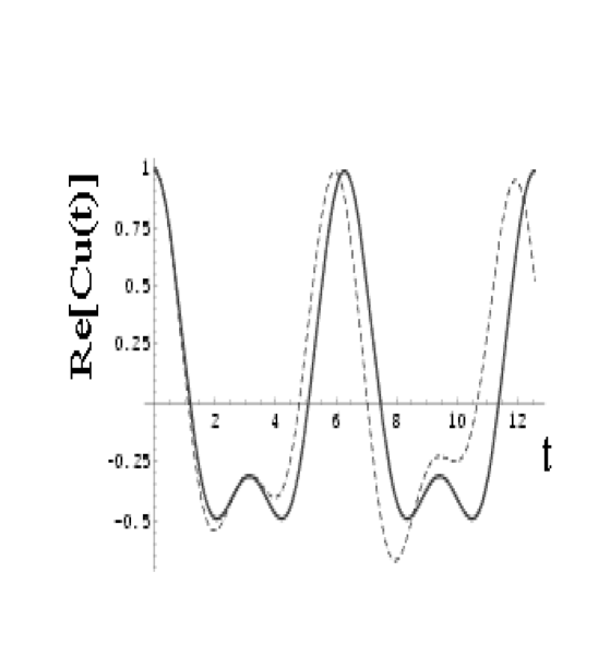
Figure 1: Time-dependence of the real part of the amplitude in the upper electronic component state. Parameter values $G=3,~{}\omega=1$. Full line: variationally obtained state. Broken line: the exact, algebraic solution.

\begin{picture}(1.0,1.0)\end{picture}

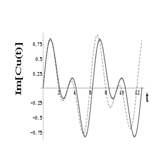
Figure 2: Same as in the previous figure but for the imaginary part of the amplitudes.

Minimizing the action with respect to the coefficients subject to the normalizing conditions turns out to be equivalent to diagonalizing a twelve-by-twelve matrix, whose elements are the action integral computed with the circular function shown in equation (28) . There are twelve-by-twelve matrix elements, rather than just six-by-six, since the upper and lower states are coupled by the off-diagonal terms in equation (25) .

We find a pair of zero eigenvalues (actually eigenvalues of about $10^{-15}$), whose meaning is the value of the action integral in the transformed representation; in other words, our variational solution is exact. Also, the numerical values of the variationally obtained coefficients $A^{u}_{g}$ agree with those in the analytic solution in equation (26) . For comparison,the other eigen solutions have ”eigenvalues” of orders 1-20.

4.1.2 A non-periodic case

With the choice of e.g., $G=3$ and $K=\frac{\sqrt{10}}{2}$, the analytic solution shown in equation (26) is not periodic and an exact solution cannot be achieved variationally while having a finite $t$-range in the action integral. Moreover, a larger spread of the basic set in equation (28) is needed. Still, so as to estimate the efficacy of the variational procedure under non-optimal conditions, we used the same $t$-range and the same set size as in (a). The lowest eigenvalues ($=$ the values of the action integral) are about $0.35$, compared with others eigenvalues, which are again in the range of 1-20.

The results are also shown graphically, by comparing the variational solution (full lines) with the exact, analytic solution (broken lines) in equation (26) for real and imaginary parts in Figures 1 and 2, respectively. The similarities are quite good for the first half (that comprises the period of the Hamiltonian), but is worse in the second half and further deteriorates later, say in the time range $({\frac{4\pi}{\omega}},{\frac{6\pi}{\omega}})$. On the other hand, had we taken the time range of the variational procedure (the upper limit of integration $T$ in equation (2) ) up to ${\frac{6\pi}{\omega}}$, we would have obviously got a somewhat different solution, which would have improved the approximation in the latter range and spoiled somewhat the agreement in the earlier range. In general, the approximate solution depends on the time-range of the action. In our view, this endows a flexibility to the practical application of the method, in the sense that, depending on which time range is of interest, better approximation can be achieved for that range. Of course, when the ”approximate” solution is identical with the true solution in some range, it will remain so, by analytical continuation, for all ranges.

In conclusion, one notes a successful application of the variational principle for a purely hermitian case, whose solution, though available by algebra, is not trivial.

4.2 A Non-linear Evolution

The continuous passage of an initially prepared pure state to transitions resembling quantum jumps was recently studied in [40], based on a form of the Liouville-von Neumann-Lindblad (LvNL) equation. The actual form used originated in a representation of fast level crossing in molecular systems involving two states [41]. It was noted in [40] that the factorization formalism, called the” square root operator” method of [25], represents an alternative way of showing how a dissipative term in the Hamiltonian can cause decoherence. To apply our variational formalism to this case, we first formulate the evolution equations in the factorization scheme and solve the resulting equations (this is done (A) below) and, secondly, we obtain an approximation to the solution by minimizing the action with respect to some parameters appearing in the assumed $\gamma$’s (this is carried out in (B)).

4.2.1 Decoherence by the ”square root operator” method

The vector potentials consisting of a Hamiltonian and a dissipative (non-Hermitian) part are now written for the two factors $(\gamma_{1},\gamma_{2})$ of the density matrix as

$${\bf A}_{1} = -\frac{1}{2}Gcos(\omega t)\gamma_{1}-J\gamma_{2}-i\Gamma[\gamma_{1}-|\gamma_{2}|^{2}(1+\mu|\gamma_{1}|^{2})/\gamma_{1}^{+}$$

$${\bf A}_{2} = \frac{1}{2}Gcos(\omega t)\gamma_{2}-J\gamma_{1}-i\Gamma[\gamma_{2}-|\gamma_{1}|^{2}(1-\mu|\gamma_{2}|^{2})/\gamma_{2}^{+}$$ (29)

One notices the similarity of these expressions with the corresponding formulae in [41] and [40] (where the interpretation of the terms is spelt out) and also the divisor $\gamma$ on the extreme right, characteristic of the factorization formalism for dissipative processes, equation (10) . The trace of the density $(\rho=\gamma{\gamma^{+}})$ stays constant during the motion and this property is maintained unchanged also by the superlinear terms which enter with the coefficient $\mu$.

It may be noted that the equations of motions for $\gamma_{1}(t)$ and $\gamma_{2}(t)$ and of their conjugates, given in equation (7) , lead to the master equations for the matrix elements of the density operator. For the diagonal elements these are of the LvNL form (when $\mu=0$), but not for the non-diagonal ones. This property has already been noticed in [25].

We next solve two equations for the $\gamma^{\prime}s$, subject to the pure state initial conditions $\gamma_{1}=1$, $\gamma_{2}=0$ at $t=0$, then form from the solutions the diagonal matrix elements of the density matrix and finally show the results in figure 3. The quantity changed between the upper three drawings is the strength $\Gamma$ of the dissipative term. As this increases, a transition takes place from the slow to the fast decoherence regime. We note the remarkable similarity of the results obtained here by the factorization method to those in Figure 1 of the above articles, except that for strong dissipation their drawings show little oscillations, unlike our third drawing from above. In this, drawn for $\frac{\Gamma}{\omega}=20$, after a very steep initial slope (not visible in the figure), both diagonal density matrix elements oscillate about the asymptotic value of $\frac{1}{2}$.

The majority of calculations whose results are shown in this section are carried out for a density matrix referring to an ”assembly” consisting of one system. This means that in Appendix A, one has $N=1$ and the summation over $\alpha$ in equation (34) is trivial. We have also worked the density matrices when there is a non-trivial summation, namely when initial conditions on the two factors are $\gamma_{1}(0)=e^{\frac{i\pi}{2}},e^{\frac{2i\pi}{2}},e^{\frac{3i\pi}{2}},e^{\frac{4i\pi}{2}}$ and $\gamma_{2}(0)=0$, (so that $N=4$), instead of having only $\gamma_{1}(0)=1$ (and $N=1$), as before. The resultant density tends now to an almost perfectly straight line. This is similar to the graphs shown in both [41] and in [40] for strong dissipation and elucidates the meaning of system-averaging in the density matrix. (In more complex systems, one would require an averaging in the density matrix over a much larger number of states, such that $N\to\infty$.) We have also worked out the $N=4$ case for the upper three graphs in figure 3. For these graphs, there was hardly any perceptible change from those shown.

For the detailed interpretation of these results, which is not the primary subject of this work, we again refer to [40, 41] and references therein. Also, we do not delve here into the details or extensions of the results, but turn to the variational treatment of time-development to be got from minimizing the action.

Figure 3: Unitary evolution. The diagonal element of the density matrix $\rho_{22}$ under a successively increasing dissipative parameter $\Gamma$. The parameters in equation (29) are $G=45$ (25 in the bottom drawing, chosen to facilitate the computation),  $J=3$, $\omega=1$,   $\mu$ (superlinearity coefficient)$=0$. Then, in top drawing: $\Gamma=0$, $N$ (Ensemble size)$=1$; in second drawing: $\Gamma=0.05$, $N=1$; in third drawing: $\Gamma=20$, $N=1$; in bottom drawing $\Gamma=20$ (as in previous, but)  $N=4$. The initial slope in the last two drawings is too steep to be visible and so are tiny fluctuations in the horizontal part of the bottom drawing. A non-zero value of the superlinear parameter $\mu$, of the order of $1$, hardly changes the curves.

4.2.2 Solving variationally

We note that the strongly oscillatory factor in the solution arises from the driving term $\frac{G}{2}cos(\omega t)$ and that this term was already present in the Hamiltonian case considered in the previous subsection, in equation (26) . (We have, however, eliminated there the fast oscillating factor by subtracting from the Hamiltonian the so-called dynamic-phase.) So in this subsection we shall put $G=0$, which also makes the numerical aspect of the variation considerably simpler. We then set up pair of suitable trial $\gamma$(t)’s, containing parameters to be varied.

In contrast to the previous subsection (which was a linear problem and in which a large number of Fourier coefficients were varied), in the present problem only one variational parameter ($v$) is introduced. However, to make progress, we must consider critical regions of the time domain, namely $t=0$ and $t=\infty$. At the former, it is easy to see that in order that the singularity due to the zero divisor ${\gamma^{+}}_{2}(0)$ in the vector potential be matched by the time derivative of $\gamma_{2}(t)$ at $t=0$, this function must take there the form of

$$\lim_{t\to 0}~{}\gamma_{2}(t)\to\sqrt{4e^{i\beta}\Gamma t}+O(t)$$ (30)

with the constant phase angle $\beta$ arbitrary. Similarly, it can be shown that, asymptotically for large $t$, the same solution must have the form

$$\lim_{t\to\infty}~{}\gamma_{2}(t)\to e^{-iJt}\sqrt{[1+ve^{-2(\Gamma-iJ)t}+o(e^{-2\Gamma t})]/2}$$ (31)

or some other form equivalent to this. A constant phase factor was ignored here. The parameter $v$ cannot be found from the equations of motion. We seek to obtain the variationally best $v$, such that the condition at $t=0$ is also satisfied. After some elementary algebra on finds that in terms of the variational parameter, the density factor $\gamma_{2}$ can have the form,

$$\gamma_{2}(t)=e^{-iJt}\sqrt{[1+ve^{-2(\Gamma-iJ)t}-(1+v)e^{-((v+2)\Gamma-ivJ)\frac{2t}{1+v}}]/2}$$ (32)

The previously introduced phase $\beta$ was varied independently and found to be small. So we put $\beta=0$. The other density factor $\gamma_{1}(t)$ was so constructed that the exponentials inside the square root had the opposite signs to those in $\gamma_{2}$ and normalizing factors were added so that $|\gamma_{1}|^{2}+|\gamma_{2}|^{2}=1$ at all times.

Minimizing the action integral for a set of parameter values for $J$ and $\Gamma$ yields optimized $v$’s. Keeping $J=3$ fixed (as in references [41, 40] and selecting a set of dissipation parameter we obtain as follows:

$J=3,~{}\Gamma=~{}0.1,~{}v~{}=~{}-.985$

$J=3,~{}\Gamma=~{}0.5,~{}v~{}=~{}-.78$

$J=3,~{}\Gamma=~{}2,~{}~{}~{}v~{}=~{}-0.755$

For the middle case $\Gamma=.5$ we compare in Figure 4. the variational solution (thin continuous curve, with $v=-.78$) and the solution from the equation of motion (thick continuous curve). In the asymptotic regime of large $t$, the behavior of the two curves is quite similar, though the amplitude of oscillation is clearly smaller in the variational solution than in the exact solution. The discrepancy appears the more serious in that a different choice of the variational parameter, namely $v=-0.98$, (also shown in the figure by broken lines), which has an action larger than the optimized one, comes nearer to the exact solution. However, we show in the inset that in the extremely short time region, the optimized solution is qualitatively better than the other choice. Because of the singular behavior of the short time region in the vector potential, this region dominates the value of the action. At the same time, yet another choice of the parameter $v=-0.05$, (shown in the figure by dotted lines) gives a definitely poorer resemblance to the correct curve.

In conclusion, when it comes to describe subtle quantum mechanical ensemble properties, the factorization (or ”square root operator”) method can be used either in its equation of motion form or variationally. In the present case, at least, the equation of motion approach was from a numerical view-point undoubtedly superior. So one may question the use of the variational method. However, on the one hand not all problems may be easily solvable. On the other hand, one should remember that the derivation of the equation of motion in equation (7) is itself based on a variational ansatz introduced in this paper.

\begin{picture}(1.0,1.0)\end{picture}

Figure 4: Comparison of solutions.   $\rho_{22}$, a diagonal component of the density matrix, for the following values of the parameters in equation 29: $G=0$, $J=3$,  $\omega=1$,  $\Gamma=0.5$, $\mu=0$. Solution of equation of motion: thick line. Variational solution in equation (32) with optimized parameter $v=-0.78$: thin line. Hypothesized solution as in equation (32) with $v=-0.98$: small broken lines. Hypothesized solution with $v=-0.05$: large broken lines. The inset shows the curves near $t=0$.

5 Further Extensions

To treat non-Markovian processes, the vector potentials have to be functions of the $\gamma$ vectors at earlier times, but otherwise, no change in the formalism is needed.

Non-negativity of the entropy-change follows from the master equations and properties of the scattering probabilities ${M_{ba}}$ in equation (12) , as is shown in [42].

Transport processes can be treated simply. Thus, let us consider electronic conduction in a solid due to a spatial gradient in the potential (i.e., an electric field) or in the ambient temperature. The $\gamma$ vectors are, normally, labeled by the reciprocal, $k$-vector index and are essentially small deviations from the square root of the equilibrium, Fermi-Dirac electronic distribution function. Following the standard treatment given in, e.g., [13], the time derivatives of the $\gamma$ vectors (that are now real and identical to $\gamma^{+}$) are proportional to the spatial gradients. The vector potentials represent the scattering integral. Then either equation of motion in equation (7) is simply the Boltzmann equation in an inhomogeneous form; namely, its left hand side represents the source or the gradient and the right hand side contains the desired distribution function under the integral over all wave-vectors. The Lagrangian can be used to obtain the solution variationally. This variational formulation is, however, different from those given in [11, 13]. (Of course, different variational procedures can lead to the same result.)

We have noted earlier that the postulated Lagrangian does not contain a potential. Adding a potential to the Lagrangian might apparently change the equations of motion. It seems to us, however, that under conditions prevailing in stochastic processes, this will not happen. The reason for this can be stated in various forms and is rooted in the circumstance (already noted above) that in the presence of a random force one has no control over the value of the variables, only on its rate of change. (”Free terminal endpoint” condition of [3], p. 9.) In Appendix B we give a formal proof for the following proposition: ”When the following conditions hold: (a) the potential is a non-negative quadratic form in all of its variables (the $\gamma$’s), (b) the vector potentials $\bf A$ are all real and positive, (c) the initial values of the $\gamma$ vectors are suitably chosen, and (d) the variation is performed under conditions of fixed initial values of $\gamma$ and ${\dot{\gamma}}$, then it follows that the action obtained from the variation of the velocities only, i.e., with the potential regarded as ignorable, is less than the action obtained from the variation of both the variables and their derivatives (namely, through the usual Lagrange equations, which are obtained under fixed initial and final boundary conditions).” The result holds probably under a wider range of conditions, since in the proof we have not utilized the requirement imposed on the self-correlation of the random forces $f_{a}$ by the ”second” theorem of Mori [43]. (This requirement ensures, among other things, the time-shift invariance of the random process which is at the root of the Onsager-Machlup theory [5, 6]. Needless to say, that the result obtained in Appendix A is not in conflict with the validity of the Euler-Lagrange equations, since these are obtained under conditions that the variables have fixed values at the final time.

6 Conclusion

The variational action (or Lagrangian) proposed in equation (2) for dynamical processes has the advantages of being simple, general and flexible. It differs from previously employed variational procedures by the factorization ansatz in equation (1) , by the absence of a scalar potential term and the presence of a variable final time upper limit. The relation of the postulated Lagrangian to some basic invariance property (like ”frame indifference” [44]) remains to be explored, account being taken of the fact that, for vector potentials that are not all equal, the formalism is non-Abelian (namely, the vector potentials cannot be transformed away by a single gauge factor)[45].

Acknowledgement

The first named author thanks S. Machlup for a discussion. The application of the formalism to a (non-linear) evolution was prompted by a referee.

Appendix A A Tutorial on the Factorized Density Matrix Formalism.

Though the factorized density matrix, written in an abstract form as $\rho={\bf\gamma}\cdot{\bf\gamma^{+}}$, has been employed before in [25] and [16], we shall explain its formalism here, following Band’s introductory texts to the von Neumann matrix method ([46],[47]). Let $\Psi_{\alpha}$ be a possible wave function describing the quantum state of the $\alpha$’th system in the ensemble $(\alpha=1,2...N)$. It can be expanded in terms of a set of eigenstates $u_{n}$ as

$$\Psi_{\alpha}=\sum_{n}\gamma^{\alpha}_{n}u_{n}$$ (33)

As derived in [46] and other texts, the density matrix arises from the ensemble average over all systems in the sense that its $nm$ component is

$$\rho_{nm}=\frac{1}{N}\sum_{\alpha}\gamma^{\alpha}_{n}\gamma^{\alpha+}_{m}$$ (34)

The $\gamma^{\alpha}$’s are best viewed as row vectors, distinct for each $\alpha$ (or system) and the $\gamma^{\alpha+}$’s as column vectors. The $\gamma$- and $\gamma^{+}$- derivatives in the text (which implement the variation procedure) are with respect to $\gamma^{\alpha}_{n}$ and $\gamma^{\alpha+}_{m}$. The ensemble averaging, namely the summing over $\alpha$ and the subsequent division by $N$, is not explicitly written out in the text, but is designated by inserting a dot between $\gamma$ symbols, so that the previous matrix element is written as

$$\rho_{nm}=\gamma_{n}\cdot\gamma^{+}_{m}$$ (35)

It is clear that the $\gamma$’s are not vector quantities, but the traces over the dotted products are proper scalars.

Appendix B Proof of the minimal action under one-point boundary condition

Assumptions: In the action, equation (2) , the vector potential $A$ is now assumed to be positive (non-negative) and real. We shall further subtract from the action (see below) a potential term, in which the potential $V$ depends on the variables only, not on their derivatives. This potential is supposed to be monotonic, non-decreasing and positive in the relevant range of its variables.

We start the proof for a single time dependent variable $g$ which replaces the earlier complex variable $\gamma$ through

$$\dot{g}=\dot{g}(t)=-i{\dot{\gamma}}$$ (36)

The reality of $g$ for all times will be evident. The one-point (initial time) boundary conditions fix $g(0)$ and ${\dot{g}(0)}$, while $g(t)$ at later times develops according to its equation of motion. We write the action, including the potential, in the single variable $g$ as

$$S(T)=\int_{0}^{T}dt[({\dot{g}}-A(t))^{2}-2V(g(t))]$$ (37)

The boundary conditions fix the value of $g(0)>0$ and of $\dot{g}(0)$. We next minimize the above action in two ways and subsequently compare the resulting actions. The first is the usual Lagrange equation way in the presence of a potential $V$ and the quantities arising from this method will be denoted by the superscript $V$. The second method pretends that there is no potential and the corresponding quantities will take the superscript $0$. It is the second method that was used in the text.

$$\ddot{g}^{V}(t)=\dot{A}(t)-V^{\prime}(g(t))$$ (38)

where the prime represents the derivative with respect to the argument $g$.

$$\dot{g}^{0}(t)=A(t)$$ (39)

The latter equation imposes the following initial condition for the velocities:

$$\dot{g}^{0}(0) = A(0)$$ (40)

$$= \dot{g}^{V}(0)$$

Integrating equation (38) once, we obtain

$$\dot{g}^{V}(t)=A(t)-P(t)\qquad P(t)\equiv\int_{0}^{t}V^{\prime}(g(t))dt$$ (41)

where $P(t)$ is zero at $t=0$ and is for positive times non-negative, since it is, by equation (38) , the time integral of a positive quantity. Subtracting $\dot{g}^{0}$ shown in equation (39) from the last equation and integrating, it is clear that $g^{V}$ never exceeds (algebraically) $g^{0}$. Calculating the actions obtained in the two methods and subtracting we find:

$$S^{V}(T) = \int_{0}^{T}dt[({\dot{g}^{V}}-A(t))^{2}-2V(g^{V}(t))]=\int_{0}^{T}dt[P(t)^{2}-2V(g^{V}(t))]$$

$$S^{0}(T) = \int_{0}^{T}dt[({\dot{g}^{0}}-A(t))^{2}-2V(g^{0}(t))]=\int_{0}^{T}dt[-2V(g^{0}(t))]$$ (42)

$$\Rightarrow S^{V}(T)-S^{0}(T)=\int_{0}^{T}dt[P(t)^{2}+2\bigl{(}V(g^{0}(t))-V(g^{V}(t))\bigr{)}]$$

In the integrand the squared term is necessarily positive (non-negative) and so is the term containing the difference of potentials since the 0-argument is larger than the V-argument and the potential is monotonic by supposition. Though obtained under restricted conditions, the result shows clearly that the two-point boundary conditions are necessary requisites for the validity of the Lagrange-Euler equations of motion. Generalization to several (real) variables $g_{1},g_{2},...,g_{N}$ is immediate, when the potential is a positive quadratic form in these variables, since this can be diagonalized (with positive eigenvalues) simultaneously with the kinetic energy term. However, the initial point variables need to be chosen carefully in this case.

Finally, we have not proven that the action using equations of motion of the text is minimal, but only that is lower than that obtained with the (for this case, inappropriate) use of the Lagrange equations. Furthermore, it is not evident that the solutions obtained in this Appendix satisfy conditions required from density matrices or probabilities (e.g., normalizations).

References

- [1] N.G. van Kampen, in L.Schimansky-Geier and T. Poschel(editors), Stochastic Dynamics, (Springer-Verlag, Berlin, 1997) p.1
- [2] J.W. Gibbs, Collected Works Vol II, Part 1, p. 1 (Yale University Press, New Haven, 1948); Am. J. Math.2 49 (1879)
- [3] B.H. Lavenda, Nonequilibrium Statistical Thermodynamics (J. Wiley, Chichester, 1985) Chapter 1
- [4] Lord Rayleigh (J.W. Strutt), Phil. Mag. 26 776 (1913)
- [5] L. Onsager and S. Machlup, Phys. Rev. 91 1505 (1953)
- [6] H. P. McKean in The Collected Works of Lars Onsager, (World Scientific, Singapore, 1996) p.769
- [7] S.R. de Groot and P. Mazur, Non-equilibrium Thermodynamics (North-Holland, Amsterdam, 1962)
- [8] H.B. Callen in I. Prigogine (editor), Proc. Int. Symp. on Transport Processes in Statistical Mechanics, (Interscience, New York, 1958) p. 327
- [9] M.J. Klein in ibid p. 311
- [10] R.P. Feynman, R.B. Leighton and M. Sands, The Feynman Lectures in Physics (Addison and Wesley, Reading, 1964) Vol.II, p. 19-14
- [11] M. Kohler, Z. Phys. 124 772 (1948); 125 679 (1949)
- [12] E.H. Sondheimer, Proc. Roy. Soc. (London) A 201 75 (1950)
- [13] J.M. Ziman, Electrons and Phonons (Clarendon Press, Oxford, 1960) Section 7.7
- [14] Ph. Blanchard, Ph. Combe and W. Zheng, Mathematical and Physical Aspects of Stochastic Mechanics, Lecture Notes in Physics (Springer-Verlag, Berlin, 1987) Chapter V
- [15] J.C. Zambrini, Intern. J. Theor. Phys. 24 277 (1985); Phys. Rev. A33 1532 (1986)
- [16] S. Gheorghiu-Svirschevski, Phys. Rev. A 63 022105 (2001);63 054102 (2001)
- [17] E. Tonti, Int. J. Engng. Sci, 22 1343 (1984)
- [18] I. Gyarmati, Non-Equilibrium Thermodynamics (Field Teory and Variational Principles) (Springer-Verlag, Berlin, 1970)
- [19] P. Van, J. Non-Equilib. Thermodyn. 21 17 (1996)
- [20] D. Djukic and B. Vujanovic, Z. Angew. Math. Mech. 51 611 (1971)
- [21] B.A. Finlayson and L.E. Scriven, Int. J. Heat Mass Transfer 10 799 (1967)
- [22] W. Muschik and R. Trostel, Z. Angew. Math. Mech. 63 T 190 (1983)
- [23] P. Kramer and M. Saraceno, Geometry of the Time-Dependent Variational Principle in Quantum Mechanics (Springer Verlag, New York, 1981)
- [24] M. Ichiyanagi, Physics Reports 243 125 (1994)
- [25] B. Reznik, Phys. Rev. Lett. 76 1192 (1996)
- [26] J. Frenkel, Wave Mechanics, Advanced General Theory (University Press, Oxford, 1934)
- [27] A.D. McLachlan, Mol. Phys. 8 39 (1964) (The concluding section of this paper notes the failure of the proposed variational method for a density matrix, when an over-simplified ansatz is used.)
- [28] A.D. McLachlan and A.M. Ball, Rev. Mod. Phys. 36 844 (1964)
- [29] J. Kucar, H.-D. Meyer andL.S. Cederbaum, Chem. Phys. Lett.140 525 (1987)
- [30] J. Broeckhove, L Lathouwers, E. Kesteloot and P. van Leuven, Chem. Phys. Lett. 149 547 (1988)
- [31] E. Deumens, A. Diz, H. Taylor and Y. Öhrn, J. Chem. Phys. 96 6820 (1992)
- [32] L. Landau and E. Lifshitz, The Classical Theory of Fields, (Addison-Wesley, Cambridge, Mass., 1951), Eq. (3-9)
- [33] R. Balian, From Microphysics to Macrophysics, (Springer Verlag, Berlin, 1992)
- [34] G.V. Chester, Repts. Prog. Phys. 26 411 (1963)
- [35] H. Lamb, Hydrodynamics, (Dover Publications, 1945)
- [36] R.L. Seliger and G.B. Whitham, Proc.Roy. Soc.(London) A 305 1 (1968)
- [37] R. Englman, A. Yahalom and M. Baer, J. Chem. Phys. 109 6550 (1998)
- [38] R. Englman, A. Yahalom and M. Baer, Europ. Phys. J. D 8 1 (2000)
- [39] R. Englman and A. Yahalom, Adv. Chem. Phys. 124 197 (2002)
- [40] A.R.P. Rau and R.A. Wendell, Phys. Rev. Lett. 89 220405 (2003)
- [41] Y. Kayanuma, Phys. Rev. B 47 9940 (1993)
- [42] N.G. van Kampen, Stochastic Processes in Physics and Chemistry, (North Holland, Amsterdam 1992) section V.5
- [43] H. Mori, Prog. Theor. Phys. 33 425 (1965)
- [44] D. Jou, J. Casas-Vazquez and G. Lebon, Extended Irreversible Thermodynamics (Springer-Verlag, Berlin, 1993) Section 1.4.1
- [45] C.N. Yang and R. Mills, Phys. Rev. 96 191 (1954)
- [46] W. Band, An Introduction to Quantum Statistics (Van Nostrand, Princeton,1955) Section 11.4
- [47] J. von Neumann, Mathematical Foundations of Quantum Mechanics (University Press, Princeton, 1955) Chapter III