The Open Path Phase for Degenerate and Non-degenerate Systems and its Relation to the Wave-function Modulus

Abstract

We calculate the open path phase in a two state model with a slowly (nearly adiabatically) varying time-periodic Hamiltonian and trace its continuous development during a period. We show that the topological (Berry) phase attains $\pi$ or $2\pi$ depending on whether there is or is not a degeneracy in the part of the parameter space enclosed by the trajectory. Oscillations are found in the phase. As adiabaticity is approached, these become both more frequent and less pronounced and the phase jump becomes increasingly more steep. Integral relations between the phase and the amplitude modulus (having the form of Kramers-Kronig relations, but in the time domain) are used as an alternative way to calculate open path phases. These relations attest to the observable nature of the open path phase.

PACS numbers: 03.65.Bz, 03.65.Ge

1 Introduction

In the last fifteen years much attention has been given to phases in wave functions and, in particular, to the topological (or Berry) phase, which is a signature of the trajectory of the system ([1]-[6]) and which is manifest in some interference and other experiments [7]. As noted in earlier works [1, 8, 9], the topological phase $\pm\pi$ that is picked up in a full revolution of the system is linked to the existence of a degeneracy of states (or crossing of potential energy surfaces) somewhere in the parameter space. This degeneracy need not be located in a region that is accessed to in the revolution; however, its removal even by a minute amount will cause the topological phase to be zero or an integral multiple of $2\pi$. The physical model treated in this work confirms this effect; indeed the calculated topological phase shows a change from $\pi$ to $2\pi$ as the degeneracy disappears (cf. Figs 1 and 2). We tackle the problem by tracing a continuous variation in the non-cyclic, open path phase [4] (also named ”connection” [2]), that is denoted in this work by $\gamma(t)$ ($t$ is time).

To obtain an expression for $\gamma(t)$ we study (for both the degenerate and non-degenerate alternatives) an explicitly solvable model. Both a detailed analysis and the figures exhibit, as a novelty, oscillations in $\gamma(t)$. These become increasingly more frequent and of lesser magnitude as the adiabatic limit is approached. Furthermore it is observed that in the adiabatic limit of the degenerate case, the change in the open path phase is abrupt and results in a step function like behavior.

In an alternative approach to the calculation of the open-path phase we develop reciprocal relations between phase and amplitude moduli of time dependent wave functions (Section 2). Versions of these relations in other contexts were given earlier ([10]-[12]). The existence of these relations has the remarkable consequence that the associated open path phase, defined by them, is a ”physical observable” (and inter alia gauge invariant) as a function of the path, a quality heretofore associated with the closed path (Berry) phase.

2 Theory

We start by invoking the Cauchy’s integral formula which takes the form:

$$w(z)=\frac{1}{2\pi i}\oint\frac{w(\zeta)}{\zeta-z}d\zeta$$ (1)

where $w(z)$ is analytic in the region surrounded by the anti-clockwise closed path. In what follows we choose the closed path to be the real axis t traversed in the reverse direction, of the infinite interval $-\infty\leq t\leq\infty$ and an infinite semi circle in the lower half of the complex plane, as will be discussed later. We shall concentrate on the case that $z$ is a real variable $t$ and so equation (1) becomes:

$$w(t)=-\frac{1}{\pi i}P\int_{-\infty}^{\infty}\frac{w(t^{\prime})}{t^{\prime}-t}dt^{\prime}+\frac{1}{\pi i}\oint_{SC}\frac{w(\zeta)}{\zeta-t}d\zeta$$ (2)

where $P$ stands for the principal value of the integral, $\zeta=\tau\exp{i\theta},d\zeta=i\tau\exp{i\theta}d\theta$ and it is assumed that $\tau\rightarrow\infty$ (the subscript $SC$ in the second term stands for semi-circle). Next it is assumed that $w(z)$ along the semi-circle is zero namely

$$\lim_{z\rightarrow\infty}w(z)=0,\qquad{\rm for}\qquad\theta\neq 0,\pi$$ (3)

so that equation (2) becomes:

$$w(t)=-\frac{1}{\pi i}P\int_{-\infty}^{\infty}\frac{w(t^{\prime})}{t^{\prime}-t}dt^{\prime}.$$ (4)

Assuming that the function $w(z)$ is written as $w(z)=w(t,y)=u(t,y)+iv(t,y)$ where $z=t+iy$, it can be shown by separating the real and the imaginary parts, that equation (4) yields the two equations:

$$u(t)=-\frac{1}{\pi}P\int_{-\infty}^{\infty}\frac{v(t^{\prime})}{t^{\prime}-t}dt^{\prime}\qquad{\rm and}\qquad v(t)=\frac{1}{\pi}P\int_{-\infty}^{\infty}\frac{u(t^{\prime})}{t^{\prime}-t}dt^{\prime}$$ (5)

These relations are of the Kramers-Kronig (KK) or dispersion equations type [13] and they will be applied in the time domain. $u$ and $v$ are Hilbert transforms [14]. Our aim is to employ equations (5) to form a relation between the phase factor in a wave function and its amplitude-modulus. If a wave-function amplitude $\tilde{\psi}(t)$ is written in the form:

$$\tilde{\psi}(t)=\tilde{\Gamma}(t)\exp(i\lambda(t))$$ (6)

where $\Gamma(t)$ and $\lambda(t)$ are real functions of a real variable $t$, the function $w(z)$ which will be defined as:

$$w(z)=\ln(\tilde{\psi}(z))=\ln(\tilde{\Gamma}(z))+i\lambda(z)$$ (7)

is assumed to fulfill the necessary conditions to employ the KK equations. This implies the following: (a) the function $\tilde{\psi}(z)$ is analytic and is free of zeroes in the lower complex half plane (however, $\tilde{\psi}(z)$ can have simple zeros on the real axis, as is made clear in several publications [10, 11, 14, 15]). (b) $\tilde{\psi}(z)$ becomes, along the corresponding infinite semi-circle, a constant (in fact this constant has to be equal to $1$ but if the constant is $\neq 1$ the analysis will be applied to $\tilde{\psi}(z)$ divided by this constant). Thus, identifying $\ln(\tilde{\Gamma}(t))$ with $u(t)$ and $\lambda(t)$ with $v(t)$ we get from the second part in equation (5) the following expression:

$$\lambda(t)=\frac{1}{\pi}P\int_{-\infty}^{\infty}\frac{\ln(\tilde{\Gamma}(t^{\prime}))}{t^{\prime}-t}dt^{\prime}$$ (8)

Next assuming that $\Gamma(t^{\prime})$ is an even function, the equation for $\lambda(t)$ can be written as:

$$\lambda(t)=\frac{2t}{\pi}P\int_{0}^{\infty}\frac{\ln(\tilde{\Gamma}(t^{\prime}))}{{t^{\prime}}^{2}-t^{2}}dt^{\prime}$$ (9)

and if $\Gamma(t^{\prime})$ is periodic then equation (9) can be further simplified to become:

$$\lambda(t)=\frac{2t}{\pi}P\int_{0}^{\tilde{T}}dt^{\prime}\ln(\tilde{\Gamma}(t^{\prime}))\sum_{n=0}\frac{1}{(t^{\prime}+N\tilde{T})^{2}-t^{2}}$$ (10)

where $\tilde{T}$ is the relevant period.

3 The Model

3.1 The Basic Equations

In this work, the reciprocal relations in equation (5) are used in the form shown in equation (10) . A more general formulation of the reciprocal relations, including several applications, will be presented in a separate publication. Equation (10) is applied to two examples based on the Jahn-Teller model [16] which, following Longuet-Higgins [17], can be expressed in terms of an extended version of the Mathieu equation, ([8, 18, 19]) namely:

$$H=-\frac{1}{2}E_{el}\frac{\partial^{2}}{\partial\theta^{2}}-G_{1}(q,\phi)\cos(2\theta)+G_{2}(q,\phi)\sin(2\theta).$$ (11)

Here $\theta$ is an angular (periodic) electronic coordinate, $\phi$ is an angular nuclear periodic coordinate which is constrained by some external agent, as in ([6], [20]), to change linearly in time, namely $\phi=\omega t$ (thus, if $T$ is the time-period, then $\omega=\frac{2\pi}{T}$), $q$ is a radial coordinate, $E_{el}$ is a constant and $G_{i}(q,\phi)$; $i=1,2$ are two functions to be defined later.

The Schrodinger equation is ($\hbar=1$):

$$i\frac{\partial\Psi}{\partial t}=H\Psi.$$ (12)

and this will be solved approximately to the first order in $\frac{qG}{E_{el}}$, for the case that the ground state is an electronic doublet. In a representation, adopted from [17], this doublet is described in terms of the electronic functions $\cos\theta$ and $sin\theta$ and therefore $\psi$ can be expressed as: ([6],[12])

$$\Psi=\chi_{1}(t)\cos\theta+\chi_{2}(t)\sin\theta$$ (13)

In what follows equation (12) will be solved for the initial conditions: $\chi_{1}(t=0)=1$ and $\chi_{2}(t=0)=0$. Replacing $\chi_{1}(t)$ and $\chi_{2}(t)$ by $\psi_{+}(t)$ and $\psi_{-}(t)$ defined as:

$$\psi_{\pm}(t)=\frac{1}{2}\exp(i\frac{1}{2}E_{el}t)(\chi_{1}\mp i\chi_{2})$$ (14)

we get the corresponding equations for $\psi_{+}(t)$ and $\psi_{-}(t)$:

$$i\dot{\psi}_{+}=-\frac{1}{2}\tilde{G}{\psi}_{-}\qquad{\rm and}\qquad i\dot{\psi}_{-}=-\frac{1}{2}\tilde{G}^{*}{\psi}_{+}$$ (15)

where $\tilde{G}$ is defined as: $\tilde{G}=G_{1}+iG_{2}$, and the dot represents the time derivative.

Next we eliminate ${\psi}_{-}$ from equation (15) to obtain a single, second order equation for $\psi_{+}$:

$$\ddot{\psi}_{+}-\dot{\ln(\tilde{G})}\dot{\psi}_{+}+\frac{1}{4}|\tilde{G}|^{2}{\psi}_{+}=0.$$ (16)

Writing $\tilde{G}=|\tilde{G}|\exp(i\Phi)$ we shall be interested in cases where $|\tilde{G}|$ is constant, so that only $\Phi$ is time-dependent. Thus equation (16) becomes:

$$\ddot{\psi}_{+}-i\dot{\Phi}\dot{\psi}_{+}+\frac{1}{4}|\tilde{G}|^{2}{\psi}_{+}=0.$$ (17)

Once equation (17) is solved we can obtain $\chi_{1}(t)$, the eigen-function for the initially populated state. Usually, this is a fast oscillating function of t where the oscillations are caused by the ”dynamical phase” $\frac{1}{2}|\tilde{G}|t$. This oscillatory component is eliminated upon multiplying $\chi_{1}(t)$ by $\exp(-\frac{1}{2}i|\tilde{G}|t)$. In what follows we consider the smoother function $\eta(t)$ defined as:

$$\eta(t)=\chi_{1}(t)\exp(-\frac{1}{2}i|\tilde{G}|t)$$ (18)

Our aim is the study of the time dependence of the phase $\gamma(t)$ defined through the expression:

$$\eta(t)=\rho(t)\exp(i\gamma(t))$$ (19)

with $\rho(t)$ and $\gamma(t)$ real. Once $\eta(t)$ is derived there are several ways to extract $\gamma(t)$ we shall use the following two: (a) the first is the following analytical representation of the open path phase given by Pati [4]:

$$\gamma(t)=\Im(\ln(\eta(t)))$$ (20)

where $\Im$ stands for the imaginary part of the expression in the parentheses. Equation (20) is used for analytical purposes, as presented below. Special emphasis will be put on $\gamma(t)$ at $t=T$ where $T$ is the period of the external field. The case of an arbitrary $T$ will be discussed only briefly and we will be mainly interested in the adiabatic case where $T$ is large, namely $T\gg|\tilde{G}|^{-1}$ for which $\gamma(t=T)$ becomes the topological (Berry) phase $\beta$. In what follows we distinguish between two cases: (a) The degenerate case for which the functions in equation (11) are given by:

$$G_{1}(q,\phi)=Gq\cos(\phi),\qquad G_{2}(q,\phi)=Gq\sin(\phi).$$ (21)

Where $G$ is constant. We term it the degenerate case because the two lowest eigenvalues of equation (11) become equal in the $(q,\phi)$ plane at $q=0$. It is also noticed that: $\tilde{G}=Gq$. (b) The non-degenerate case. This is characterized by the condition that $G_{1}=0$ and $G_{2}=0$ cannot be simultaneously satisfied for real $q$ and $\phi$.It is not trivial to achieve this by a simple change of the expressions in equation (21) , since, e.g., adding a constant will only displace the real root, as has been previously discussed [19]. However, non-degeneracy can be attained upon replacing $G_{2}$ by a quadratic polynomial in $q\sin(\phi)$, such that the polynomial has no real roots. A term of this form is physically realizable in a low-symmetric molecular environment. (In a realistic case of non crossing potential energy surfaces for NaFH, the expression constructed for $G_{2}$ is very complicated [21]). Unfortunately, the equation (16) cannot be solved analytically for a general polynomial $G_{2}$. Below (in section 4) we present an approximate solution for a case that a degeneracy is encountered neither at $q=0$ nor at any other real $q$-value. This is achieved by the choice:

$$G_{1}(q,\phi)=Gq\cos(\phi),\qquad{\rm and}\qquad G_{2}(q,\phi)=\sqrt{(Gq)^{2}\sin^{2}(\phi)+\mu^{2}}$$ (22)

The quantity $\mu$ is related to the separation between the two potential energy surfaces.

If we expand the square root for small $q$, we indeed recover a quadratic polynomial approximation, that has no real roots. It is noticed that now $|\tilde{G}|=\sqrt{G_{1}^{2}+G_{2}^{2}}=\sqrt{(Gq)^{2}+\mu^{2}}$. In what follows it is assumed for simplicity that the particle trajectory is on the circle $q=1$.

3.2 The Degenerate Case

We start by considering the degenerate case and therefore in equation (16) $\Phi\equiv\phi=\omega t$ and $|\tilde{G}|=G$ as already mentioned, (see equation (21) ). As a result, equation (17) becomes:

$$\ddot{\psi}_{+}-i\omega\dot{\psi}_{+}+\frac{1}{4}G^{2}{\psi}_{+}=0.$$ (23)

The solution of this equation (as well as that of a similar equation for ${\psi}_{-}(t)$) can be written in terms of trigonometric functions. Returning to the original $\chi$-functions we get for $\chi_{1}(t)$ the following explicit expression:

$${\chi_{1}} = \cos(kt)\cos(\frac{1}{2}\omega t)+\frac{\omega}{2k}\sin(kt)\sin(\frac{1}{2}\omega t)$$ (24)

$$+ i\frac{G}{2k}\sin(kt)\cos(\frac{1}{2}\omega t)$$

where $k$, defined as:

$$k=\frac{1}{2}\sqrt{G^{2}+\omega^{2}}$$ (25)

forms, together with $\omega$, two characteristic periodicities of the system.

\begin{picture}(1.0,1.0)\end{picture}

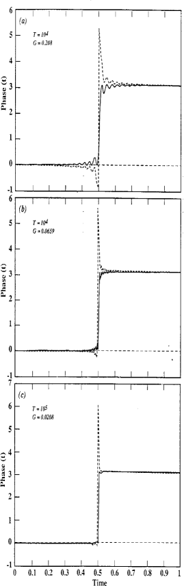
Figure 1: The time-dependent phase factor $\gamma$ as a function of time calculated for the degenerate case. The calculations were done for different values of the external field frequency $\omega(=\frac{2\pi}{T})$, and the coupling intensity $G$. In all three cases the Rabi oscillations are of a time period $(\frac{2\pi}{k})$ where $k$ is defined as $k=\frac{1}{2}\sqrt{G^{2}+\omega^{2}}$. In each sub-figure two curves are shown; one, drawn as a full line, is the curve calculated employing equation (24) and the other, drawn as a dashed line, is the approximate curve calculated employing the Kramers-Kronig relation shown in equations (8-10) and (32). (a) $T=10^{4}$, $G=0.01$. (b) $T=10^{4}$, $G=0.02$. (c) $T=10^{5}$, $G=0.01$.

In Fig. 1 are shown several $\gamma(t)$-functions as calculated for three different values of $G$ and $T(=\frac{2\pi}{\omega})$. It is noticed that as $T$ increases, namely as the adiabatic limit is approached, $\gamma(t)$ tends to a step function and $\beta$- the Berry phase- reaches the value of $\pi$. This behavior is also derived analytically as follows.

Considering the case that $T\rightarrow\infty$ (or $\omega\rightarrow 0$), one can show employing equations (20) and (24) for the adiabatic case, that $\gamma(t)$ takes the form (discarding second order terms in $\omega$):

$$\lim_{T\rightarrow\infty}(\gamma(t))=\Im\{\ln[\cos(\frac{1}{2}\omega t)+O(\omega)]\}$$ (26)

Having this expression it is recognized that since $\cos(\frac{1}{2}\omega t)>0$ for $t\leq\frac{T}{2}$ and $\cos(\frac{1}{2}\omega t)<0$ for $t\geq\frac{T}{2}$ it follows that $\gamma(t)\simeq 0$ for $0\leq t\leq\frac{T}{2}$ and $\gamma(t)\simeq\pi$ for $\frac{T}{2}\leq t\leq T$. This also implies that the topological (Berry) phase $\beta\simeq\pi$. From Fig. 1 it is noticed that, when the adiabatic limit is approached (namely, $T\rightarrow\infty$), $\gamma(t)$ becomes a step function. The step takes place at $t\sim\frac{T}{2}$. It is therefore of interest to study the behavior of $\gamma(t)$ in the vicinity of $t=\frac{T}{2}$. Thus expanding $\gamma(t)$ around this value and keeping only first order terms in $(t-\frac{T}{2})$ yield:

$$\gamma(t\approx\frac{T}{2})=\Im\{\ln[\frac{T}{2}-t+\frac{1}{k}\sin kt\exp(ikt)]\}$$ (27)

It is noticed that around $t=\frac{T}{2}$ the phase factor $\gamma(t)$ oscillates (Rabi oscillations) and its periodicity is $(\frac{2\pi}{k})$. These oscillations become more frequent the larger is the value of the product $GT(\gg 1)$.

In order to obtain the phase using equation (10) we have to construct from $\chi_{1}(t)$, which when analytically continued to the complex plane becomes $\chi_{1}(z)$, a new function that fulfills the requirements imposed on $\tilde{\psi}(z)$. The complex function $\chi_{1}(z)$ is obtained by replacing in equation (24) , the variable $t$ by $z$ defined as:

$$z=\tau\exp(i\theta);\qquad{\rm where}\qquad 0\leq\theta\leq 2\pi\qquad{\rm and}\qquad\tau>0.$$ (28)

The first requirement imposed on $\tilde{\psi}(z)$ is that it does not have zeros in the lower half plane. The newly formed function $\chi_{1}(z)$ has, in general, zeros in the lower half plane. But we have been able to show generally that near the adiabatic limit there are no zeros for the ground state in the lower half plane. [Moreover, a detailed numerical study showed that when the ratio of inverse periods $(\frac{k}{\omega})=$ integer, the zeros (of the ground state) are located in the upper half plane (including the real axis). For the near adiabatic situation where $(\frac{k}{\omega})$ is large, the requirement $\frac{k}{\omega}=$ (a large) integer can (on physical grounds) differ only insignificantly from neighboring values of $\frac{k}{\omega}$ that are non integral. We thus have two independent reasons for the assertion regarding the location of zeros in the near adiabatic case. This is also confirmed by our graphical results in Figures 1 and 2, which clearly show the increasing validity of the integral relations, as the adiabatic limit is approached, upon going from (a) to (c), and this even though the ratio $(\frac{k}{\omega})$ is not chosen to be an integer.] The second requirement imposed on $\tilde{\psi}(z)$ is that it becomes equal to $1$ along the infinite semi-circle on the lower half of the complex plane. From equation (24) it is readily seen that for $\tau\rightarrow\infty$ the function $\chi_{1}(z)$ in the adiabatic limit becomes (for $\theta>\pi$):

$$\lim_{\tau\rightarrow\infty}\chi_{1}(z)=\frac{1}{2}\exp(i(k+\frac{1}{2}\omega)\tau e^{i\theta})$$ (29)

or

$$\lim_{\tau\rightarrow\infty}\chi_{1}(z)=\frac{1}{2}\exp(-(k+\frac{1}{2}\omega)\tau\sin\theta)\exp(i(k+\frac{1}{2}\omega)\tau\cos\theta)$$ (30)

Therefore multiplying $\chi_{1}(z)$ by $2\exp(-i(k+\frac{1}{2}\omega)\tau e^{i\theta})$ yields the function $\tilde{\psi}(z)$ which becomes equal to $1$ along the infinite-semi circle. Thus the function to be employed in equation (10) is $\tilde{\psi}(t)$ defined as:

$$\tilde{\psi}(t)=2\chi_{1}(t)\exp(-i(k+\frac{1}{2}\omega)t)$$ (31)

Combining Eqs. equation (8) , equation (10) , equation (18) , equation (19) and equation (31) we obtain the final expression for the phase $\gamma(t)$ up to a linear function of time that follows from the KK equations:

$$\gamma(t)=\frac{2t}{\pi}P\int_{0}^{\tilde{T}}dt^{\prime}\ln(\tilde{\Gamma}(t^{\prime}))\sum_{n=0}\frac{1}{(t^{\prime}+N\tilde{T})^{2}-t^{2}}$$ (32)

where $\tilde{\Gamma}(t)$ is is absolute value of $\chi_{1}(t)$. It is important to emphasize that $\tilde{T}$ is not necessarily equal to $T$ (in our particular case $\tilde{T}$ is equal to $2T$). In Fig. 1 is presented $\gamma(t)$ also as calculated from equation (32) . The results along the interval $0\leq t\leq(\frac{T}{2})$ were taken as they are but those along the interval $\frac{T}{2}\leq t\leq T$ were found to be $2\pi$ below the values obtained by the direct method. We added to each of the calculated values the physically unimportant magnitude $2\pi$. The comparison between the curves due to the two different calculations reveals a reasonable fit which improves when either T or G become large enough, namely upon approaching the adiabatic limit. Even the (Rabi) oscillations at the near adiabatic limit are well reproduced by the present theory. Moreover the theory yields the correct geometrical phase. It is also important to mention that when we are far from the adiabatic limit the fit is less satisfactory. However, we also found that for the choices of $k$ which make the function $\chi_{1}(t)$ periodic, namely when $(\frac{k}{\omega})=$ integer, the agreement resurfaces [12].

4 The Non-Degenerate Case

This arises when $\mu\neq 0$ (see equation (22) ). As a result we obtain for $|\tilde{G}|$, $\Phi$ and $\dot{\Phi}$ the following expressions:

$$|\tilde{G}|=\sqrt{G^{2}+\mu^{2}};\qquad\Phi=\arccos(p\cos\omega t);\qquad\dot{\Phi}=p\omega\frac{\sin\omega t}{\sqrt{1-p^{2}\cos^{2}\omega t}}$$ (33)

where $p$ is defined as $p=\frac{G}{\sqrt{G^{2}+\mu^{2}}}$. In what follows we consider only the case when $\mu$ is small enough so that $|\tilde{G}|$ and $\Phi$ are, as before, equal to $G$ and $\omega t$, respectively, but $\dot{\Phi}$ will be written as: $\dot{\Phi}=\omega\frac{\sin\omega t}{|\sin\omega t|}$. Thus equation (17) becomes:

$$\ddot{\psi}_{+}\mp i\omega\dot{\psi}_{+}+\frac{1}{4}|\tilde{G}|^{2}{\psi}_{+}=0.$$ (34)

where the minus sign is for the $0\leq t\leq(\frac{T}{2})$ - the first half period and the plus sign for $\frac{T}{2}\leq t\leq T$ - the second half. For the first half we have the same equation as before and therefore also the same solution (see equation (24) ). As for the second half period we obtain a somewhat more complicated expression for the solution due to the matching of the two solutions at $t=\frac{T}{2}$. Thus:

$$\chi_{1}(t) = e^{-i\pi}\{\cos(kt)\cos(\frac{1}{2}\omega t)-\frac{\omega}{2k}\sin(k(T-t))\sin(\frac{1}{2}\omega t)$$ (35)

$$+ i\frac{G}{2k}\sin(kt)\cos(\frac{1}{2}\omega t)\}$$

$$- \frac{\omega}{2k^{2}}\sin(\frac{kT}{2})\sin(k(t-\frac{1}{2}T))[\omega\cos(\frac{1}{2}\omega t)+iG\sin(\frac{1}{2}\omega t)]$$

In order to obtain the phase factor for the adiabatic case, equation (20) is applied as before, where $\chi_{1}(t)$ is given by equation (35) . We employed equation (35) to calculate $\gamma(t)$ based on the KK dispersion relations.

Figure 2: The time dependent phase factor $\gamma$ as a function of time calculated for the non-degenerate case. Details as in Fig.1. The approximate curve was calculated employing equations (8-10) and (32) for $0\leq t\leq(\frac{T}{2})$ and equations (8-10) and (35) for $\frac{T}{2}\leq t\leq T$. (a) $T=10^{4}$, $G=0.01$. (b) $T=10^{4}$, $G=0.02$. (c) $T=10^{5}$, $G=0.01$.

In Fig. 2 are presented the results due to the two types of calculations as obtained for three sets of values of the parameters $G$ and $T$. It is noticed that when either $T$ or $G$ become large enough (namely, approaching the adiabatic limit), as in the previous case, a reasonably good fit is obtained between the results due to the direct calculations and the ones based on the KK relations (equations (10) and (35)). Moreover, in this case, too, this new formalism yields the correct geometrical phase.

The same analytic treatment can be done for the non-degenerate two-state model. Considering again the case that $T\rightarrow\infty$ (or $\omega\rightarrow 0$), but for equation (35) , we obtain that $\gamma(t)$ takes the form:

$$\lim_{T\rightarrow\infty}(\gamma(t))=\Im\{\ln[\cos(\frac{1}{2}\omega t)+O(\omega)]\}+\Theta(t-\frac{T}{2})\pi$$ (36)

where $\Theta(x)$ is the Heavyside function defined as being equal to zero for $x<0$ and equal to $1$ for $x>0$. It is noticed that the sign of the expression in the square brackets is positive for $0\leq t\leq\frac{T}{2}$ which means that the phase factor is altogether zero (because also $\Theta(x)=0$) but the sign is positive for $\frac{T}{2}\leq t\leq T$ and therefore altogether $\gamma(t)=2\pi$ and this leads to a topological (Berry) angle $\beta=2\pi$. This result is expected because the Berry phase has to be zero (or $2\pi$) in the case of no degeneracy.

5 Conclusions

The expression of the degeneracy and near-degeneracy dichotomy in the topological phase is the main subject of this paper. The respective values of $\pi$ and $2\pi$ after one revolution (seen in Figures 1 and 2, respectively) obtained in a two-stage model confirm the expectations. However, on the way to this result we earned some new results and insights. Oscillations near the half period stage were found (equation (27) ) and explained. We also studied the tendency of this and of other features in the ”connection” (namely the non-cyclic phase) with the approach to adiabatic (slow) behavior.

An attempt has been made in this article to establish a link between the time dependent phase (and its particular value, the topological phase, after a full revolution) with the corresponding amplitude modulus. To establish this relation we considered two alternative two-state models, exposed to an external field, under adiabatic and quasi-adiabatic conditions ([3], [19]). The two types of models are physically different: (a) one model contains an (ordinary Jahn-Teller type) degeneracy at a point in configuration space; (b) the second is characterized by a nearly (in fact, non-)degenerate situation (of the pseudo-Jahn-Teller type([16])) where the two eigenvalues approach each other at some point in configuration space but do not touch. In Figs. 1 and 2 are presented time dependent phases and the (Berry) topological phases for these two models calculated in two different ways: once directly by employing equation (20) and once by using the KK relations which led to equation (10) . Essentially these findings suggest that one may be able to obtain the time dependence of the phase from a series of time-dependent measurements of relative populations of a given state. We end by offering the following interpretation for our findings: The phase on the left-hand side of equations (8-10) is not a ”physical observable” in the conventional sense since no hermitian operator is associated with it [10]. Yet, phases have been observed in interference and other experiments [7]. In the present formulation, equations . (8-10) associate the observable phase of the wave function with $\Gamma(t)$ (the observable probability amplitude) through integral expressions, in a similar way to that done in Ref. [11] for radiation fields.

References

- [1] M.V. Berry, Proc. R. Soc. London, Ser. A 392, 45 (1984).
- [2] B. Simon, Phys. Rev. Lett. 51, 2167 (1983).
- [3] Y. Aharonov & J. Anandan, Phys. Rev. Lett. 58, 1593 (1987).
- [4] A.K. Pati, Phys. Rev. A 52, 2576 (1995); S.R. Jain and A.K. Pati, Phys. Rev. Lett. 80, 650 (1998).
- [5] C.M. Cheng & P.C.W. Fung, J. Phys. A Math. Gen. 22, 3493, (1989).
- [6] D.J. Moore & G.E. Stedman, J. Phys. A Math. Gen. 23, 2049 (1990).
- [7] T. Bitter & D. Dubbens, Phys. Rev. Lett. 59, 251 (1998); D. Suter, K.T. Mueller & A. Pines, Phys. Rev. Lett. 60, 1218 (1988); H. von Busch, Vas Dev, H.-A. Eckel, S. Kasahara, J. Wang, W. Demtroder, P. Sebald & W. Meyer, Phys. Rev. Letters 81, 4584 (1998).
- [8] R. Englman & M. Baer, J. Phys. C: Condensed Matter 11, 1059 (1999).
- [9] R. Resta & S. Sorella, Phys. Rev. Letters 74, 4738 (1995). (Especially bottom of first column on p. 4740).
- [10] L. Mandel & E. Wolf, Optical Coherence and Quantum Optics Sections 3.1 and 10.7 (University Press, Cambridge, 1995); L. Mandel & E. Wolf, Rev. Mod. Phys. 37, 231 (1965).
- [11] J.H. Shapiro & S. R. Shepard, Phys. Rev. A 43, 3795 (1991) (Footnote 53).
- [12] R. Englman, A. Yahalom & M. Baer, Phys. Lett. A 251, 223 (1999).
- [13] H.M. Nussenzweig , Causality and Dispersion Relations pages 24, 212 (Academic Press, NewYork, 1972).
- [14] E.C Titchmarsh, The Theory of Functions Sections 7.8 and 8.1 (Clarendon Press, Oxford, 1932).
- [15] R. Englman & A. Yahalom, Phys. Rev. A (1999, Submitted).
- [16] R. Englman, The Jahn-Teller Effect in Molecules and Crystals (Wiley Interscience, London, 1972).
- [17] H.C. Longuet-Higgins, Adv. Spectrosc. 2, 429 (1961).
- [18] M. Baer & R. Englman, Mol. Phys. 75, 293 (1992); R. Baer, D. Charutz, R. Kosloff & M. Baer, J. Chem. Phys. 105, 9141 (1996).
- [19] M. Baer, A. Yahalom & R. Englman, J. Chem. Phys. 109, 6550 (1998).
- [20] J.W. Zwanziger & E.R. Grant, J. Chem. Phys. 87, 2954 (1987).
- [21] M.S. Topaler, D.G. Truhlar, X.Y. Chang, P. Piecuch & J.C. Polanyi, J. Chem. Phys. 108, 5349 (1998).