Rotational cooling of heteronuclear molecular ions with ${}^{1}\Sigma\;$, ${}^{2}\Sigma\;$, ${}^{3}\Sigma\;$and ${}^{2}\Pi\;$electronic ground states

Abstract

The translational motion of molecular ions can be effectively cooled sympathetically to translational temperatures below 100 mK in ion traps through Coulomb interactions with laser-cooled atomic ions. The ro-vibrational degrees of freedom, however, are expected to be largely unaffected during translational cooling. We have previously proposed schemes for cooling of the internal degrees of freedom of such translationally cold but internally hot heteronuclear diatomic ions in the simplest case of ${}^{1}\Sigma\;$electronic ground state molecules. Here we present a significant simplification of these schemes and make a generalization to the most frequently encountered electronic ground states of heteronuclear molecular ions: ${}^{1}\Sigma\;$, ${}^{2}\Sigma\;$, ${}^{3}\Sigma\;$and ${}^{2}\Pi\;$. The schemes are relying on one or two laser driven transitions with the possible inclusion of a tailored incoherent far infrared radiation field.

I Introduction

The cooling and manipulation of neutral molecules has become the subject of intense studies in recent years and impressive advances have been made. Experiments include the successful production of molecular Bose-Einstein condensates Jochim et al. (2003); Zwierlein et al. (2003); Greiner et al. (2003), the deceleration and trapping of polar molecules in inhomogeneous fields Bethlem et al. (2002); van de Meerakker et al. (2001); Crompvoets et al. (2002); Bethlem and Meijer (2003) and loading a trap with paramagnetic molecules cooled by a He buffer gas Weinstein et al. (1998); Egorov et al. (2002). For the NH radical the presence of an unusually large Franck-Condon factor offers prospects for direct Doppler cooling of a trapped molecule van de Meerakker et al. (2003).

Molecular ions constitute another class of molecules that are very interesting to cool and manipulate. Diatomic molecular ions are, e.g., important constituents of interstellar media Snow (1992); Snyder (1992), comets and cool stellar atmospheres including that of the sun Snyder (1992); Wegmann et al. (1999), and there have recently been proposals to utilize cold molecules to implement a quantum computer Demille (2002); Tesch and de Vivie-Riedle (2002).

The cooling of molecules is in general more complicated than that of atoms since the ro-vibrational substructure of the electronic molecular energy levels normally makes it impossible to find a closed optical pumping scheme to be used for conventional laser cooling. Molecular ions, however, may be very effectively cooled sympathetically by loading them into a trap with laser cooled atomic ions Mølhave and Drewsen (2000); Drewsen et al. (2003); Schiller and L mmerzahl (2003); Fr hlich et al. ; van Eijkelenborg et al. (1999). The Coulomb interaction between the charged particles provides efficient momentum transfer from the initially hot molecular ions to the cooled atomic ions. Dissipative cooling of the translational motion is hence obtained for both species although only the atomic ions are subject to laser cooling.

One might expect that the ro-vibrational degrees of freedom of a diatomic molecule placed in the vicinity of a cooled atomic ion would couple to the translational motion of the atomic ion, resulting in strong sympathetic cooling of these degrees of freedom. In a typical ion trap, however, the excitation energy of the translational atomic motion in the trap (vibrations in the harmonic trap potential) is of the order of 1 MHz, which is much smaller than typical energies of ro-vibrational excitations (of the order $10^{11}-10^{14}$ Hz). The large difference between these numbers prohibits that the internal ro-vibrational states couple effectively to the external motion of the ions in the trap. In the following we therefore assume that the internal degrees of freedom relax to equilibrium with the black-body radiation (BBR) present in the trap. This will happen on a timescale of tens of seconds, which is significantly faster than the inelastic collision time in the trap which, from Langevin theory, is estimated to be hundreds of seconds Vogelius et al. (2002).

In Refs. Vogelius et al. (2002, 2004) we proposed schemes for cooling of the rotational degree of freedom of such molecular ions in the case of heteronuclear molecules with a ${}^{1}\Sigma\;$electronic ground state. The schemes are based on two direct infrared (IR) transitions between the lowest vibrational states in the molecule or two Raman transitions coupling the vibrational levels via a near-resonant excited electronic state. In addition to the pumping by the external light sources the cooling schemes are assisted by rotational redistribution mediated by the BBR. The timescale of the cooling schemes are on the order of $\sim 60$ s which is shorter than the estimated inelastic collision rate with background gas.

Though most molecules appearing in nature have a ${}^{1}\Sigma\;$electronic ground state it is necessary to consider other electronic states for molecules produced in the laboratory, including molecular ions. The by far most frequently encountered electronic ground states of such molecules and molecular ions are, apart from the ${}^{1}\Sigma\;$state, the ${}^{2}\Pi\;$, ${}^{2}\Sigma\;$and ${}^{3}\Sigma\;$states. This includes the lighter diatomic hydrides, e.g., FH${}^{+}\,$(${}^{2}\Pi\;$), BH${}^{+}\,$(${}^{2}\Sigma\;$) and OH${}^{+}\,$(${}^{3}\Sigma\;$). Such ionized hydrides are attractive candidates for our cooling schemes as they have low reduced masses and hence high rotational transition frequencies leading to fast rotational relaxation rates which is beneficial for the timescale of the cooling scheme. By extending the schemes to ${}^{2}\Pi\;$, ${}^{2}\Sigma\;$and ${}^{3}\Sigma\;$states we have then covered all the lighter ionic hydrides and the vast majority of other molecules amenable for cooling. We show that it is possible to cool such electronic states, though at the cost of introducing more laser frequencies in some cases. For most molecules, however, the present cooling schemes rely on only a single IR laser, possibly assisted by broadband radiation from a far-infrared (FIR) emitter which is filtered to optimize the cooling efficiency.

The present paper is organized as follows. In Sec. II we present cooling schemes for the ${}^{1}\Sigma\;$electronic ground states. In Sec. III we discuss a model of the cooling schemes and present numerical simulations for MgH${}^{+}\,$(X${}^{1}\Sigma$). In Sec. IV we present cooling schemes applicable to the ${}^{2}\Sigma\;$, ${}^{3}\Sigma\;$and ${}^{2}\Pi\;$electronic ground states together with numerical simulations of each of the cooling schemes. A summary of the results is given in Sec. V. In Appendix A, we have collected the Einstein coefficients for the considered molecules and transitions, and in Appendix B, we describe the Hönl-London factors of interest.

II Cooling schemes for ${}^{1}\Sigma\;$states

The suggested schemes for ${}^{1}\Sigma\;$states are sketched in Fig. 1. The driven transitions are either Raman transitions via an excited electronic state or transitions directly between vibrational levels. Fig. 1(a) represents the cooling scheme of Ref. Vogelius et al. (2002) in which two Raman transitions make a closed cycle through pumping of population from the “pump states”, $(\nu=0,N=1)$ and $(\nu=0,N=2)$, to the excited states, $(\nu=1,N=1)$ and $(\nu=1,N=0)$, respectively, followed by subsequent spontaneous emission bringing the populations back to the “pump states” or to the ro-vibrational ground state. Here $\nu$ and $N$ denotes the vibrational and rotational level respectively. Population initially in higher-lying states is fed to the pump states through BBR–induced rotational transitions within the vibrational ground state.

It would be advantageous for practical implementation to use only a single Raman (Fig. 1(b)) or a single direct (Fig. 1(c)) transition, at the expense of not emptying the $(\nu=0,N=1)$ state. Without applying other means to limit the pile-up of population in the $(\nu=0,N=1)$ state the cooling efficiency, measured as the percentage of population in the ground state, will decrease. One can, however, take advantage of the higher frequency of the $(\nu=0,N=1)\leftrightarrow(\nu=0,N=2)$ rotational transition compared to the undesired $(\nu=0,N=0)\rightarrow(\nu=0,N=1)$ heating transition inevitably driven by the BBR, and apply an incoherent source and a high-frequency pass filter to reduce the radiation resonant with the heating transition while still addressing the $(\nu=0,N=1)\leftrightarrow(\nu=0,N=2)$ transition. Thereby one can obtain the desired depletion of the $(\nu=0,N=1)$-population by means of incoherent radiation only. As the rate of depletion using realistic incoherent sources will be slower than if the state was addressed by a laser, it is necessary to design the cooling scheme such that spontaneous decays to the $(\nu=0,N=1)$ state from states which are participating in the pumping cycle are avoided. This can be done by addressing the $(\nu=0,N=2)\leftrightarrow(\nu=2,N=0)$ transition with a resonant, dipole allowed ($\Delta N=0,\pm 2$) Raman pulse as depicted in Fig. 1(b). The pumping to the $(\nu=2,N=0)$ state is then followed by spontaneous decays through $(\nu=1,N=1)$ to $(\nu=0,N=0)$ and $(\nu=0,N=2)$ in accordance with the dipole selection rules $((\Delta N,\Delta\nu)=\pm 1)$ for single photon decays.

It is shown in Ref. Vogelius et al. (2002) that the Raman-transitions in the MgH${}^{+}\,$test case Mølhave and Drewsen (2000) are saturated by a $\sim 100$ kW/cm², $10$ ns pulse, which is a modest intensity for present day laser systems.

One of our schemes using only a single direct laser-induced transition subject to the dipole selection rule is shown in Fig. 1(c) Vogelius et al. (2004). The laser pumps the $(\nu=0,N=2)\leftrightarrow(\nu=1,N=1)$ transition while subsequent spontaneous decay brings the population back to the pump state or to the ro-vibrational ground state. A filtered incoherent source is applied in order to bring population from the $(\nu=0,N=1)$ state to the ”pump state”. The advantage of this direct scheme is that it does not depend on the existence of an excited electronic state that can be addressed with laser light and also that it requires only a single laser frequency. ArH${}^{+}\,$is an example of a molecule without excited electronic states Schutte (2001); Vogelius et al. (2002).

From a practical point of view, a pulsed laser system is desirable for the direct scheme of Fig. 1(c). The IR light could, for example, be generated by difference frequency mixing of the primary beam of a frequency doubled Nd:YAG laser and a dye laser pumped with the same beam. In the MgH${}^{+}\,$case, the wavelength of the $(\nu=0,N=2)\leftrightarrow(\nu=1,N=1)$ pumping transition is $\simeq 5.9\ \mu$m Huber and Herzberg (1979) and the Einstein A-coefficient is $\simeq 20$ s^-1. To ensure saturation of the laser driven transition we require that the population in the states involved undergoes at least 10 Bloch oscillation during a laser pulse and that the amplitude of each oscillation exceeds $0.9$. If we assume a detuning of $1$ GHz and a pulse duration $10$ ns we find that an intensity of $\sim 500$ W/mm² is needed to fulfill both requirements. This corresponds to a pulse energy of 5 $\mu$J. Typical nonlinear crystals should be able to deliver an energy of $\sim 10$ $\mu$J per laser pulse at the wavelength required.

The added incoherent field from a lamp will increase the rate of rotational transitions needed for cooling, but at the expense of heating the population distribution. The spectral distribution of the incoherent field can therefore be shaped to maximize the cooling efficiency as described in Ref. Vogelius et al. (2004).

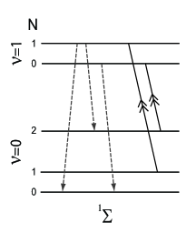
(a) Cooling scheme of Ref. Vogelius et al. (2002)

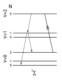
(b) Raman scheme

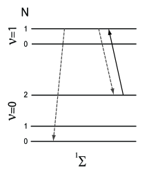
(c) Direct scheme

Figure 1: Ro-vibrational states of interest in the cooling schemes for ${}^{1}\Sigma\;$states. The cooling concept involves transitions between ro-vibrational states driven by Raman pulses (solid lines, double arrows in (a) and (b)) via an excited electronic state or direct laser pumping (solid line, single arrow in (c)) and subsequent spontaneous decays (dashed lines).

III Numerical simulations for ${}^{1}\Sigma\;$states

In this section, we present our model of the cooling scheme, show the results of numerical simulations and discuss the optimal radiation distribution of the incoherent field.

III.1 Rate equations for the population dynamics

The population dynamics is well-described by rate equations giving the change in population of a given state via Einstein coefficients and frequency-specific radiation intensities. The equation of motion for the molecular population $P_{i}$ in state $i$ takes the form

$$\begin{split}\frac{dP_{i}}{dt}=&-\sum_{j=0}^{i-1}A_{ij}P_{i}+\sum_{j=i+1}^{M}A_{ji}P_{j}-\\ &\sum_{j=0}^{i-1}P_{i}B_{ij}W(\omega_{ij})+\sum_{j=0}^{i-1}P_{j}B_{ji}W(\omega_{ij})-\\ &\sum_{j=i+1}^{M}P_{i}B_{ij}W(\omega_{ij})+\sum_{j=i+1}^{M}P_{j}B_{ji}W(\omega_{ij}).\end{split}$$ (1)

Here

$$\begin{gathered}\bm{P}=(P_{\nu=0,N=0},P_{\nu=0,N=2}\ldots P_{\nu=0,N=N_{max}},P_{\nu=1,N=0}\\ \ldots P_{\nu=1,N=N_{Max}},P_{\nu=2,N=0}\ldots P_{\nu=2,N=N_{max}})\end{gathered}$$ (2)

represents the populations in vector form with $N_{max}$ chosen so the population in higher-lying rotational states is negligible during the cooling process. $A_{ij}$ and $B_{ij}$ are the Einstein coefficients describing spontaneous and stimulated transitions from energy level $i$ to $j$. $W(\omega_{ij})$ is the cycle averaged radiative energy density present in the trap at the resonant transition frequency $\omega=\omega_{ij}$, between level $i$ and $j$. In Eq. (1), the first term corresponds to spontaneous decay from state $i$ to states with lower energy, while the second term describes spontaneous decay from levels with higher energy into state $i$. Stimulated emission from the $i$th state and stimulated absorption from lower-lying states is then described by the third and fourth term, and finally, the last two terms represent transitions due to absorption of radiation from the $i$th state and stimulated emission from higher-lying states into the $i$th state.

The system of Eqs. (1) is conveniently expressed by the matrix equation

$$\frac{d\bm{P}}{dt}=\bm{K}\bm{P},$$ (3)

where $\bm{K}$ is an $(M+1)\times(M+1)$ coupling matrix.

III.2 Calculation of molecular properties

As seen from Eq. (1), it is necessary to know the Einstein coefficients to simulate the population dynamics. For many molecules, the Einstein coefficients are available in the literature. If not, they are evaluated numerically as follows. We use the well-known quantum mechanical expressions for the Einstein coefficients between an upper state $\Psi_{n}$ and a lower state $\Psi_{m}$ that are both non-degenerate Loudon (1983)

$$\begin{split}B_{n,m}&=\frac{\pi|\bm{D}_{n,m}|^{2}}{3\epsilon_{0}\hbar^{2}},\\ A_{n,m}&=\frac{\hbar\omega^{3}}{\pi^{2}c^{3}}B_{n,m},\end{split}$$ (4)

where $\omega$ denotes the transition frequency and $\bm{D}$ the transition dipole moment between the states.

$$\bm{D}_{n,m}^{lab}=\int\Psi_{n}^{\ast}\bm{M}^{lab}\Psi_{m}d\tau,$$ (5)

with $d\tau$ denoting the volume element corresponding to integration over the complete set of coordinates for all particles involved and

$$\bm{M}^{lab}=\sum_{k}-e\bm{r}_{k}+\sum_{l=1,2}Z_{l}e\bm{R}_{l}$$ (6)

the dipole operator.

The equations refer to a laboratory-fixed coordinate system so the molecular wave-functions include the rotational terms. The summation indices in Eq. (6), k and l, refer to the electrons and the involved nuclei, while $Z_{l}$ denotes the nuclear charge.

For degenerate states Eq. (4) is modified to

$$\begin{split}B_{n,m}&=\frac{\pi|\mathcal{D}_{n,m}|^{2}}{3g_{n}\epsilon_{0}\hbar^{2}}\\ A_{n,m}&=\frac{\hbar\omega^{3}}{\pi^{2}c^{3}}B_{n,m},\end{split}$$ (7)

where dipole matrix elements connecting ro-vibrational levels, $\mathcal{D}_{n,m}$, are derived in Appendix B.

$$|\bm{\mathcal{D}}_{m,n}|^{2}=S_{J_{m},J_{n}}\Big{|}\int f_{\nu_{n}}(R)D_{e}(R)f_{\nu_{m}}(R)R^{2}dR\Big{|}^{2}.$$ (8)

The Hönl-London factors, $S_{J_{m},J_{n}}$, are tabulated in the literature Huber and Herzberg (1979); Tatum (1966); Kovács (1969); Whiting et al. (73) and may be evaluated by the expressions given in Appendix B. Both the potential energy curve for the molecule and the electronic dipole moment function $\bm{D}_{e}^{mol}(R)$ is evaluated with Gaussian Frisch et al. (1995). From the potential energy curve the ro-vibrational eigenfunctions, $f_{\nu_{n}}$, are readily found using the Numerov method, and the one-dimensional integral of Eq. (8) can be evaluated. We use the Level 7.5 program LeRoy (2002) to perform these tasks and to evaluate Eq. (7), leaving us with the desired Einstein coefficients.

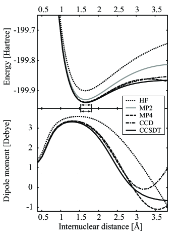
Figure 2: Top: Born-Oppenheimer electronic potential energy curves of MgH${}^{+}\,$(X${}^{1}\Sigma$) calculated by Gaussian in a 6-311++G basis set Foresman and Frisch (1996) using Hartree-Fock (HF) theory, Møller-Plesset nth order perturbation theory (MPn), coupled cluster theories with singles and double excitations (CCD), and single, double and triple excitations (CCSDT). See Refs. Møller and Plesset (1934); Bauschlicher and Langhoff (1991); Lawley (1987); Krishnan and Pople (1978); Pople et al. (1987) for descriptions of the methods. The curves for the MP4, CCD and CCSDT calculations are in good agreement close to the equilibrium position, $1.65$Å, indicating that these methods give an accurate description of the problem. Bottom: Corresponding dipole moment functions, $\bm{D}_{e}^{mol}(R)$ of Eq.(23) pointed along the internuclear axis, of MgH${}^{+}\,$calculated with Gaussian. The MPn and coupled cluster theories largely agree around the equilibrium distance, although not as well as for the potential curve due to the dependence on electronic wave functions rather than eigenenergies. The classical turning points for the vibrational ground state are marked on the common abscissa at $~{}1.5$ and $1.8$ Å. The result of the MP2 calculation cannot be discriminated from the MP4 result at the internuclear distances of interest.

III.2.1 Einstein coefficients for MgH${}^{+}\,$

Since translational cold samples of MgH${}^{+}\,$have been produced in a trap loaded with laser cooled Mg⁺ atomic ions Mølhave and Drewsen (2000), this molecular ion is the first choice for an implementation of the presented cooling schemes. To our knowledge only a few Einstein coefficients for transitions within the electronic ground state have been published Vogelius et al. (2002). We have re-calculated the coefficients using the approach of the previous section. The potential curves obtained from Gaussian Frisch et al. (1995) using various theoretical approaches on a 6-311++G basis set Foresman and Frisch (1996) is given in Fig. 2 together with the corresponding dipole moment functions in the molecular center of mass system. The potential curves show convincing convergence and our derived vibrational transition frequencies and equilibrium distance agree with published data within 1.5$\%$ Huber and Herzberg (1979). To compute the accurate electronic dipole moment function is more challenging, since this requires accurate electronic wave functions. Generally the M ller-Plesset fourth-order perturbation theory Krishnan and Pople (1978) and the coupled-cluster theories Pople et al. (1987) are reliable for the task. The dipole moment functions converge against a unique function as the level of approximation is refined as shown in Fig. 2 indicating that the highest order CCSDT function is a good approximation to the physical dipole moment function. Furthermore, we have performed equivalent calculations on the isoelectronic molecules NaH and BeH⁺ Zemke et al. (1984); Ornellas et al. (1983); Machado and Ornellas (1991) to compare our results with other published calculations. The results were in agreement within 5$\%$, a level which is not critical for the simulations of the cooling schemes. The calculated Einstein coefficients are given in appendix A.

We have now set up the model and acquired the parameters entering the coupling matrix $\bm{K}$ in Eq. (3) and the solution can now be found numerically using standard methods as described below.

III.3 Solving the population dynamics

We model the dynamics of the cooling on the test case of MgH${}^{+}\,$by solving Eq. (3) Dormand and Prince (1980). In the population vector, $\bm{P}$, of Eq. (2) we use $N_{max}=20$ since the population of this and higher-lying levels is effectively zero during the cooling process. In addition, we omit the $(\nu=2,N)$ states in the cooling schemes if the second excited vibrational state is not coupled by laser fields. The radiation density $W(\omega)$ at resonance between levels not addressed by lasers has been calculated from a Boltzmann distribution at $300$ K plus incoherent fields from lamps as described below. The pulsed lasers are included by saturating the pumped transitions, described in Sec. II, at a repetition rate of $100$ Hz. In the simulation this is done by redistributing the population in the involved ro-vibrational levels at the given repetition rate according to the degeneracy of the levels. All simulations are made with populations which are initially Boltzmann distributed at a temperature of 300K. The shape of the incoherent field is chosen so it maximizes the final population in the rovibrational ground state.

All simulations are made with the most abundant isotopes, in this case ²⁴Mg¹H⁺ (79%).

III.4 Efficiency of ${}^{1}\Sigma\;$cooling schemes

In Ref. Vogelius et al. (2004) we found that the optimized radiation density at intermediate timescales induces transitions up to and including the peak of the population distribution in BBR alone at 300K. Specifically, for MgH${}^{+}\,$the optimized spectral distribution of the incoherent source used in the schemes of Fig. 1(b) and 1(c) is found to be a square distribution with the maximal density allowed on the rotational transitions from $(\nu=0,N=1)\leftrightarrow(\nu=0,N=2)$ to $(\nu=0,N=3)\leftrightarrow(\nu=0,N=4)$. Furthermore, we showed that the spectral radiation density reaching the molecular ions from a realistic lamp is approximately 5 times the spectral radiation energy density of BBR at 300K. This has been included as a constraint in the optimization of the incoherent field.

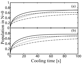
Figure 3: Population in the ro-vibrational ground state of MgH${}^{+}\,$(X${}^{1}\Sigma$) vs. cooling time for the Raman (a) and direct (b) schemes presented in Figs. 1(b) and (c) with the optimized distribution of incoherent radiation (solid), quartz-filtered distribution (dashed) and no incoherent source (dash-dot). The same simulation using the scheme of Fig. 1(a) is depicted for comparison (dot).

While the cooling efficiency at a given time depends critically on the ability to filter out radiation addressing the heating transition in the low-frequency end of the distribution, it is only weakly depending on the sharpness of the filter in the high-frequency end. This is illustrated in Figs. 3 and 4 by the inclusion of a simulation using a square incoherent field addressing the transitions $(\nu=0,N=1)\leftrightarrow(\nu=0,N=2)$ to $(\nu=0,N=7)\leftrightarrow(\nu=0,N=8)$ roughly corresponding to the cutoff frequency of a crystalline quartz window Kimmitt (1970). This distribution will be referred to as the ”quartz-filtered” distribution below. Simulations of the evolution of ro-vibrational ground state population of MgH${}^{+}\,$during cooling with the direct and Raman scheme using these two incoherent fields are presented in Fig. 3 together with the results obtained without the inclusion of an incoherent source and those obtained by applying the scheme of Ref. Vogelius et al. (2002) (Fig. 1(a)).

For very short cooling times no significant difference between the schemes is seen as the relatively slow rotational transitions have not yet set in. On intermediate time-scales the effect of the added incoherent field is evident and the optimized scheme has an advantage to the scheme of Ref. Vogelius et al. (2002) at times less than $\sim 100$ s. At long times the slower depletion of the $(\nu=0,N=1)$ state using the incoherent field rather than a laser, as well as the heating effect of the added radiation makes the scheme of Ref. Vogelius et al. (2002) more effective than the other schemes.

The schemes presented here has the advantage of reaching significant cooling after $\sim 30$ s which, combined with the modest demands to coherent light sources, makes them experimentally attractive. Anticipated performance of traps for neutrals give storage times exceeding 10 s, comparable to the timescale of the cooling schemes applied on MgH${}^{+}\,$van de Meerakker et al. (2001) and in the same regime as ArH${}^{+}\,$, which is a faster candidate Vogelius et al. (2002). Hence the application of the schemes may be considered to create rotationally cold neutral molecules in the presence of BBR.

The population distribution after 60 s of cooling is compared with the initial Boltzmann distribution in Fig. 4. The depletion of the rotational levels above the $N=2$ “pump state” is evident. The difference between using the optimized and quartz-filtered spectral distribution of incoherent light can be seen in the figures, but the effect is very limited.

The final population in the ro-vibrational ground state of just below 80$\%$, c.f. Fig. 4, corresponds to the ground state population of a thermal ensemble of MgH${}^{+}\,$at $\sim$7 K.

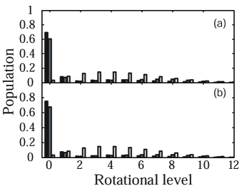
Figure 4: Population distribution in MgH${}^{+}\,$(X${}^{1}\Sigma$) after 60 s of cooling using the Raman (a) and direct (b) schemes with the optimized energy distribution of the incoherent source (black), the quartz-filtered energy distribution (gray), compared to the initial population distribution at 300 K (white). The ground state population after cooling with the optimized incoherent field corresponds to that of a thermal ensemble at $\sim 7$K.

IV Cooling scheme for molecules with rotational sub-structure

In the previous sections, we discussed cooling schemes applicable to molecular ions with their ro-vibrational energy levels determined by molecular rotation and vibration only. This will be the case if the relevant electronic state has vanishing total spin and if the projection of the orbital angular momentum of the electronic state along the internuclear axis is zero, i.e., in ${}^{1}\Sigma\;$states. We now turn to the other electronic ground states found in lighter diatomic hydride ions: ${}^{2}\Sigma\;$, ${}^{3}\Sigma\;$and ${}^{2}\Pi\;$

A range of quantum numbers will be needed to describe the rotational sub-states of the molecules to be discussed. We follow the notation of Herzberg Huber and Herzberg (1979) designating the quantum numbers as indicated in Table 1. The meaning of the coupled angular momenta is explained below.

Table 1: Overview of quantum numbers describing the rovibrational state of a molecule, neglecting nuclear spin. $\hat{\bm{\zeta}}$ denotes a unit vector along the internuclear axis.

Label	Definition
$\bm{L}$	Total electronic orbital angular momentum
$\Lambda$	Projection of $\bm{L}$ on internuclear axis
$\bm{N}$	Angular momentum of molecular rotation
$\bm{S}$	Total electronic spin
$\Sigma$	Projection of $\bm{S}$ on internuclear axis
$M_{S}$	Projection of $\bm{S}$ on laboratory Z-axis
$\Omega$	$\Lambda+\Sigma$
$\bm{K}$	Sum of $\bm{N}$ and $\Lambda\cdot\hat{\bm{\zeta}}$
$\bm{J}$	Total angular momentum of molecule neglecting nuclear spin
$M_{J}$	Projection of $\bm{J}$ on laboratory Z-axis

We now treat Hunds coupling case (a) and (b) separately and study cooling schemes for both cases.

IV.1 ${}^{(2S+1)}\Pi$-states; Hunds case (a)

An interaction term of the form $H^{so}=A\bm{L}\cdot\bm{S}$ will appear in the Hamiltonian if the projection on the internuclear axis of both electronic spin, $\bm{S}$, and electronic orbital angular momenta, $\bm{L}$, are nonzero. For moderate rotational excitations this will normally dominate over terms from the rotational Hamiltonian, $H^{rot}=B\cdot\bm{N}^{2}$. It is therefore convenient to choose the Hunds case (a) basis set, consisting of basis functions $\left\lvert{n,\bm{S}^{2}\bm{J}^{2}M_{J}\Lambda\Sigma\Omega}\right\rangle$ where $n$ is collecting the quantum numbers defining the molecular state but not mentioned in Table 1. In this basis set, the unperturbed Hamiltonian, $H_{0}$ is diagonal and the main perturbation term $H^{so}$ is nearly diagonal with the off-diagonal terms satisfying $\Delta\Omega=0$. The $\left\lvert{n,\bm{S}^{2}\bm{J}^{2}M_{J}\Lambda\Sigma\Omega}\right\rangle$ basis states are therefore a good approximation to eigenfunctions with good quantum numbers if $|A|\gg B\cdot J$. In the following section, we restrict the calculation to the pure Hunds case (a) limit where this condition is fulfilled. ${}^{2}\Pi\;$states are often close to this limit at low rotational excitations and they form the most interesting example of Hunds case (a) coupling for our purpose, as they are found as ground states of a number of molecules interesting for cooling, including NH${}^{+}\,$and FH${}^{+}\,$.

IV.1.1 Energy levels and selection rules

The first order effect of $H^{so}$ is to split the electronic ground state into states according to the value of $\Omega$. For each of these states there will be a set of ro-vibrational sub-states arising from $H^{rot}$.

In Hunds case (a), the molecule is well-described as a rotating symmetric top, for which the rotational energies are expressed by Huber and Herzberg (1979)

$$F_{\nu}(J)=B_{\nu}(J(J+1)-\Omega^{2}).$$ (9)

Here $J$ must take values greater than $|\Omega-N|$ and the lowest rotational state will therefore, in general, have $J\neq 0$. The overall structure of the molecular energy levels can be seen from the sketch of the modified cooling scheme in Fig. 5 for $S=\frac{1}{2}$.

The case (a) basis state in the laboratory frame can be written as a Wigner rotation of the corresponding wave function in the molecular rest frame Hornkohl and Parigger (1996)

$$\begin{split}&\left\langle{\{\bm{r}_{i}\}\bm{R}|nJM_{J}\Omega S\Sigma}\right\rangle=\\ &\sqrt{\frac{2J+1}{8\pi^{2}}}\left\langle{\{\bm{r}_{i}^{\prime}\}R|n}\right\rangle\left\lvert{S\Sigma}\right\rangle\mathcal{D}_{M_{J}\Omega}^{J^{\ast}}(\alpha\beta\gamma),\end{split}$$ (10)

where $\{\bm{r}_{i}\},\bm{R}$ ($\{\bm{r}_{i}^{\prime}\},R$) are the electronic and internuclear coordinates in the laboratory (body-fixed) frame. Finally $\mathcal{D}_{M\Omega}^{J^{\ast}}(\alpha\beta\gamma)$ is an element of the Wigner rotation matrix evaluated at the given Euler angles, $\alpha\beta\gamma$ Brink and Satchler (1994). The Hönl-London factors $S(J^{\prime},J^{\prime\prime})$ are found as outlined in Appendix B

$$\begin{gathered}S(J^{\prime},J^{\prime\prime})=(2J^{\prime\prime}+1)\times\\ |\left\langle{J^{\prime\prime}\Omega^{\prime\prime}1(\Omega^{\prime}-\Omega^{\prime\prime})|J^{\prime}\Omega^{\prime}}\right\rangle|^{2}\delta_{S^{\prime},S^{\prime\prime}}\delta_{\Sigma^{\prime},\Sigma^{\prime\prime}},\end{gathered}$$ (11)

where $\left\langle{J^{\prime\prime}\Omega^{\prime\prime}1(\Omega^{\prime}-\Omega^{\prime\prime})|J^{\prime}\Omega^{\prime}}\right\rangle$ is a Clebsch-Gordan coefficient. This result immediately gives us the following dipole selection rules

$$\Delta J = 0,\pm 1\quad\textrm{but}\quad J=0\nleftrightarrow J=0$$

$$\Delta\Lambda = 0,\pm 1,$$ (12)

$$\Delta S = \Delta\Sigma=0,$$

which can also be combined to $\Delta\Omega=0$.

IV.1.2 Cooling schemes

For ${}^{2}\Pi\;$molecules we propose the cooling scheme depicted in Fig. 5, where we distinguish between the possible values of $\Omega=\frac{1}{2}$ and $\Omega=\frac{3}{2}$. Since only transitions with $\Delta J=0,\pm 1$ are allowed, we can pump population from the first excited rotational state in the vibrational ground state to the rotational ground state of the first excited vibrational level. The former is denoted the ”pump state” in analogy with the nomenclature in Sec. II. From the $(\nu=1,J=\Omega)$ state spontaneous emission brings population either back to the pump state or down to the ro-vibrational ground state. The cooling scheme must be applied for each populated $\Omega$ state individually. In Fig. 5 we have assumed population of both $\Omega=\frac{1}{2}$ and $\Omega=\frac{3}{2}$. In the absence of incoherent radiation this forms a pumping cycle where population initially in the $(\nu,J)=(0,\Omega+1)$ state is transferred to the ro-vibrational ground state. As in the singlet case, the presence of BBR and possibly additional incoherent radiation from a lamp, will induce rotational transitions and thereby feed the pump state with population from higher-lying states. The entire population is therefore cooled.

Cooling schemes for other Hunds case (a) molecules may be derived from straightforward generalization of the ${}^{2}\Pi\;$scheme.

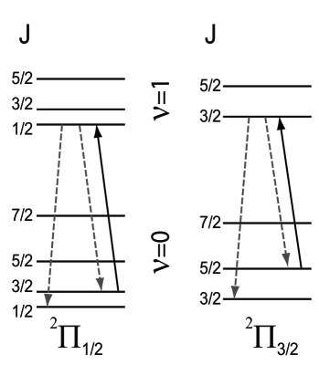
Figure 5: Cooling scheme for ${}^{2}\Pi$-states. Each of the two possible values of $\Omega$ results in a series of energy levels and it is necessary to cool the ${}^{2}\Pi_{\frac{1}{2}}$ and ${}^{2}\Pi_{\frac{3}{2}}$ separately if both are populated. Population is pumped from the first excited rotational state in the $\nu=0$ vibrational ground state to the ro-vibrational ground state by a laser induced vibrational transition and subsequent spontaneous decays. All the involved transitions are dipole allowed, cf., Eq. (IV.1.1). Solid lines indicate laser pumped transitions while dashed lines indicate spontaneous decay paths. The $\Lambda$ doubling is not shown in the figure.

IV.1.3 Numerical simulations

The simulation is done using the approach described in Sec. III.3 but with the dipole transition matrix elements calculated using the Hönl-London factors of Eq. (11). We have chosen the molecule FH${}^{+}\,$as an example of a ${}^{2}\Pi\;$ground state molecule.

Since the spin-orbit coupling parameter $A=-292$ cm^-1 is much larger in magnitude than the rotational constant $B=17$ cm^-1 FH${}^{+}\,$is best described in the Hunds case (a) scheme Coe et al. (1989). The appropriate cooling scheme is depicted in Fig. 5, although it should be noted that, for FH${}^{+}\,$, $\Omega=\frac{3}{2}$ is the lower state. To model the cooling scheme we use the dipole moment functions in Ref. Werner et al. (1984) and the accurate spectroscopic data of Ref. Coe et al. (1989).

In the cooling scheme of Fig. 5 the pumping is done from the first excited rotational level. This fact, combined with a large permanent dipole moment and hence rotational transition rate of FH${}^{+}\,$(2.57 Debye), makes the effect of the broadband incoherent radiation marginal. We have therefore performed the simulations without the inclusion of an incoherent source. The results of simulations are given for both the ${}^{2}\Pi\;$_1/2 and ${}^{2}\Pi\;$_3/2 states in Figs. 6 and 7.

Further splitting of the levels indicated in Fig. 5 will appear due to $\Lambda$ doubling. The effect is largest in the ${}^{2}\Pi\;$${}_{\frac{1}{2}}$ state where it has a magnitude on the order of 10 GHz, which is more than one can expect to cover with the bandwidth of a single pulsed laser. Therefore the laser transitions indicated for the ${}^{2}\Pi\;$${}_{\frac{1}{2}}$ scheme needs to be divided into two. The splitting of the lowest ${}^{2}\Pi\;$${}_{\frac{3}{2}}$ state is an order of magnitude smaller, so it is not necessary to split that laser transition if a pulsed laser system is used. This leaves us with three laser frequencies to use for the cooling scheme if we assume that both $\Omega=\frac{1}{2}$ and $\Omega=\frac{3}{2}$ are populated.

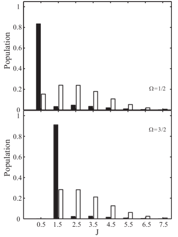
Figure 6: Cooling efficiency of FH${}^{+}\,$(X${}^{2}\Pi$) in the two $\Omega$ sub-states. In the dipole approximation the two sub-states are uncoupled if pure Hunds case (a) applies. The cooling scheme will therefore be significantly simplified if one can design the experiment such that only the lowest $\Omega=\frac{3}{2}$ state is populated in the cooling scheme

Complications arise if we are not in the pure Hunds case (a) scheme. This occurs if the rotational part of the Hamiltonian cannot be neglected compared to the spin-orbit part. Treated in the case (a) basis, the rotational part will produce non diagonal perturbations Lefebvre-Brion and Field (1986). This would allow a coupling from $(\nu=1,J=\Omega)\rightarrow(\nu=0,J=\Omega+2)$ (the introduction of quadrupole couplings would have a similar effect). We do not expect this effect to be significant given the difference between $|A|$ and $B$. We did, however, check the stability of the scheme when introducing such couplings and found that due to the fast rotational redistribution rates, the population that was coupled out of the cooling cycle by $\Delta J=2$ transitions would rapidly be taken back. The negative effect of such couplings is small (less than 10% decrease in cooling efficiency) if the $\Delta J=\pm 2$ couplings are less than 20% of the $\Delta J=0$ coupling strength.

It should be noted that since the coupling between the $\Omega$ states is also absent in the pure case (a) coupling, it would be possible to prepare the sample so that only the $\Omega=\frac{3}{2}$ sub-state is populated, due to its significantly lower energy. This would make the lasers addressing the other level superfluous. In that case only a single laser frequency is needed to cool the molecules.

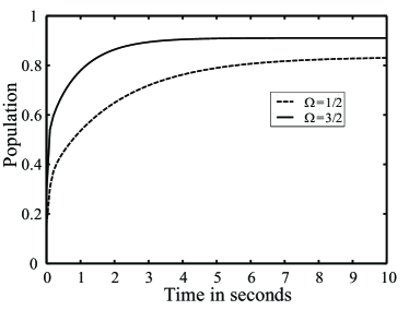
Figure 7: Cooling efficiency as function of cooling time for the two $\Omega$ sub-states of the ${}^{2}\Pi\;$electronic ground state of FH${}^{+}\,$. The cooling is seen to reach steady-state after $\lesssim 10$ s without the inclusion of an incoherent source, largely due to the large permanent dipole moment of FH${}^{+}\,$.

IV.2 ${}^{(2S+1)}\Sigma$-states; Hunds case (b)

If $B\gtrsim|A|$ or at high rotational excitations the Hunds case (a) basis functions will no longer be approximate energy eigenfunctions. If $H^{rot}$ dominates, the Hunds case (b) basis, $\left\lvert{n\bm{J}^{2}M_{J}\bm{N}^{2}\bm{S}^{2}\Lambda}\right\rangle$ is convenient as the total Hamiltonian is nearly diagonal in this basis. In particular this is fulfilled for ${}^{2S+1}\Sigma$ states which are common as electronic ground states of light diatomic molecular ions, including BH${}^{+}\,$(X${}^{2}\Sigma$) and OH${}^{+}\,$(X${}^{3}\Sigma$). Below we treat the ${}^{2}\Sigma\;$and ${}^{3}\Sigma\;$cases separately.

IV.2.1 Energy levels of doublet states

The sub-states of a rotational level in a molecule in a ${}^{2}\Sigma\;$state are split due to the interaction of the spin of the unpaired electron and the molecular rotational angular momentum. This is due to the spin-rotation Hamiltonian, $H^{sr}=\gamma\bm{N}\cdot\bm{S}$, with $\gamma$ denoting the spin-rotation coupling constant. The resulting energies of the doublet are given by Huber and Herzberg (1979)

$$F_{1}(N) = BN(N+1)+\frac{1}{2}\gamma N,$$ (13)

$$F_{2}(N) = BN(N+1)-\frac{1}{2}\gamma(N+1),$$ (14)

and the sub-states are denoted $F_{1}$ and $F_{2}$ for $J=N+\frac{1}{2}$ and $J=N-\frac{1}{2}$ respectively.

IV.2.2 Energy levels of triplet states

Molecular ions in ${}^{3}\Sigma\;$electronic states will, apart from the spin-rotation splitting discussed above, have an additional splitting from the coupling of the electronic spin of the two unpaired electrons. Such states are relatively rare, as pairing of the electronic spins is usually favored. Nevertheless, the ionic hydrides in the 16th group of the periodic table, including OH${}^{+}\,$and SH${}^{+}\,$, have such electronic ground states and we therefore consider the applicability of the cooling schemes to such states here. The energies of the three spin sub-states are given by Huber and Herzberg (1979)

$$F_{1}(N) = BN(N+1)+\frac{2\lambda(N+1)}{2N+3}+\gamma(N+1),$$ (15)

$$F_{2}(N) = BN(N+1),$$ (16)

$$F_{3}(N) = BN(N+1)-\frac{2\lambda N}{2N-1}-\gamma N.$$ (17)

In analogy with the doublet case $F_{1}$, $F_{2}$, and $F_{3}$ denotes the sub-states with $J=N+1$, $J=N$ and $J=N-1$, respectively. In the expression $\gamma$ is the spin-rotation coupling constant and $\lambda$ is the spin-spin–splitting constant. The latter is normally an order of magnitude or more larger than $\gamma$ and, consequently, the multiplet splitting of triplet states at moderate rotational excitations are much greater than the corresponding splittings of a doublet electronic states.

IV.2.3 Selection rules

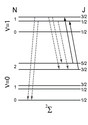
Figure 8: Cooling scheme for ${}^{2}\Sigma$-states. Due to the spin-rotation coupling each rotational quantum state $N$ split into two sub-levels with $J=|N+\frac{1}{2}|,|N-\frac{1}{2}|$. The dipole-allowed vibrational transitions are indicated on the figure using solid lines for laser pumped transitions and dashed lines for subsequent spontaneous decay paths.

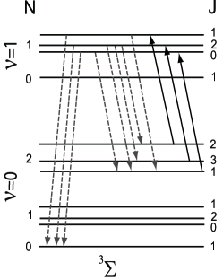
Figure 9: Cooling scheme for ${}^{3}\Sigma$-states. Due to spin-spin and spin-rotation coupling each rotational quantum state $N$ split into sub-levels with $J=|N+1|,N,|N-1|$. The dipole-allowed vibrational transitions are included in the figure with solid lines to indicate laser pumped transitions and dashed lines to indicate spontaneous decay paths.

In Hunds case (b) the good quantum numbers are $N,S,J,M_{J}$ and $\Lambda$. We therefore write the eigenfunctions in the laboratory frame as

$$\begin{gathered}\left\langle{\{\bm{r}_{i}\},\bm{R}|nJM_{J}NS,\Lambda}\right\rangle=\sqrt{\frac{2N+1}{8\pi^{2}}}\times\\ \sum_{M_{S}=-S}^{S}\sum_{M_{N}=-N}^{N}\left\langle{\{\bm{r}_{i}^{\prime}\},R|n}\right\rangle\left\langle{NM_{N}SM_{S}|JM_{J}}\right\rangle\times\\ \left\lvert{SM_{S}}\right\rangle\mathcal{D}_{M_{N}\Lambda}^{N^{\ast}}(\alpha\beta\gamma),\end{gathered}$$ (18)

where $\{\bm{r}_{i}\},\bm{R}$ ($\{\bm{r}_{i}^{\prime}\},R$) are the electronic and internuclear coordinates in the laboratory (body-fixed) frame. We then follow the approach of Appendix B to get the Hönl-London factors

$$\begin{gathered}S(J^{\prime},J^{\prime\prime})=(2N^{\prime\prime}+1)(2J^{\prime}+1)(2J^{\prime\prime}+1)\times\\ \left\langle{N^{\prime\prime}\Lambda^{\prime\prime}1(\Lambda^{\prime}-\Lambda^{\prime\prime})|N^{\prime}\Lambda^{\prime}}\right\rangle^{2}\begin{Bmatrix}S^{\prime}&N^{\prime\prime}&J^{\prime\prime}\\ 1&J^{\prime}&N^{\prime}\end{Bmatrix}^{2}\delta_{S^{\prime}S^{\prime\prime}},\end{gathered}$$ (19)

where $\begin{Bmatrix}S^{\prime}&N^{\prime\prime}&J^{\prime\prime}\\ 1&J^{\prime}&N^{\prime}\end{Bmatrix}$ is a 6j symbol Brink and Satchler (1994). The following selection rules are extracted

$$\begin{split}\Delta J&=0,\pm 1\quad\textrm{but}\quad J=0\nleftrightarrow J=0\\ \Delta N&=0,\pm 1\quad\textrm{but }\ \Delta N\neq 0\quad\textrm{if $\Lambda^{\prime}=\Lambda^{\prime\prime}=0$}\\ \Delta\Lambda&=0,\pm 1,\\ \Delta S&=0.\end{split}$$ (20)

IV.2.4 cooling scheme

The cooling scheme proposed for Hunds case (b) molecules closely resembles the singlet cooling scheme. It is depicted in Fig. 8 for ${}^{2}\Sigma\;$molecules and in Fig. 9 for ${}^{3}\Sigma\;$molecules. The optical pumping is done from the $(\nu=0,N=2,J)$ set of states to $(\nu=1,N=1,J^{\prime})$. Then dipole allowed spontaneous decay will result in transitions back to the ”pump states” or to the non-degenerate ro-vibrational ground state. The only change to the scheme when compared to the singlet case is to assure the addressing of all sub-states in the $N$ multiplet. This is possible because the $\Delta N=\pm 1$ selection rule for $\Sigma$ states from Eq. (20) is the same as in the singlet case. The role of BBR and additional incoherent radiation is the same as in the previous schemes.

The number of transitions to be pumped is three for the ${}^{3}\Sigma\;$states and two for the ${}^{2}\Sigma\;$states. The splitting of the levels in the former is expected to be much larger than for the ${}^{2}\Sigma\;$case, since the spin-spin coupling parameter $\lambda$ is much greater than the spin-rotation parameter $\gamma$ as mentioned in Sec. IV.2.

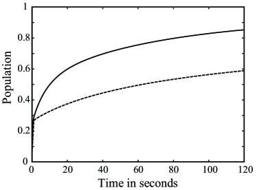
Figure 10: Population in the lowest rotational state of BH${}^{+}\,$(X${}^{2}\Sigma$) as function of cooling time. Simulations are made using the scheme of Fig. 8 with BBR only (dashed line) and with the inclusion of the field from an incoherent source addressing the $N=1\rightarrow N=2$ and $N=2\rightarrow N=3$ transitions (solid line). We see that a significant improvement is obtainable using the incoherent source. In line with our experience from MgH${}^{+}\,$there is only a couple of percent loss of cooling efficiency when using a softer low-frequency pass filter, for example, letting the broadband incoherent radiation extend to include transitions up to and including $N=4\rightarrow N=5$.

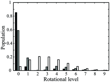
Figure 11: Population in the lowest rotational states of BH${}^{+}\,$(X${}^{2}\Sigma$) after cooling in 120 s using the incoherent radiation from a lamp addressing the $N=1\rightarrow N=2$ and $N=2\rightarrow N=3$ transition (Black columns) and in BBR only (grey columns). The initial 300K Boltzmann distribution is included for comparison (unfilled columns). We note that slightly better cooling efficiency should can be obtained using longer cooling times, cf Fig. 10. This is, however, impractical and the obtainable improvements would be rather small. The substructure of the rotational levels is included in the simulation but omitted on the figure.

IV.2.5 Numerical simulations; BH${}^{+}\,$(${}^{2}\Sigma\;$)

Here we treat BH${}^{+}\,$as an example of a ${}^{2}\Sigma\;$ground state molecule and discuss the molecule specific parameters and their implications on the cooling schemes.

The numerical simulation is done for ¹¹B¹H⁺ which is the dominant isotope (80%). We use the potential energy and dipole moment functions of Ref. Klein et al. (1982). With those functions, we use the approach of Sec. IV.2.3 to calculate the matrix of Einstein coefficients between rotational and vibrational states. Finally, we make the simulation as described in Sec. III.3 but with the modified energy level structure. If one neglects fine-structure, the laser wavelength for the two, then identical, pump transitions depicted in Fig. 8, is $\Omega_{0}=4.17\mu$m. The real resonant transition frequencies are shifted from this central frequency through Eq. (13) where $\gamma=-0.014$ cm^-1 Huber and Herzberg (1979). This gives a splitting of laser frequencies, including fine structure, of $\pm 0.007\>$cm${}^{-1}\simeq\pm 210\>$MHz. This difference is comfortably smaller than the typical bandwidth of a pulsed laser system. The hyperfine coupling coefficient has, to our knowledge, not been calculated. Typical values are, however, on the order tens to hundreds of MHz, allowing us to address all hyperfine substates with the same pulsed laser system. Hence, it is reasonable to expect that for practical implementations only a single, pulsed laser frequency is needed.

The results of a numerical simulation are given in Figs. 10 and 11. We note that the convergence is quite slow compared to what we saw from MgH${}^{+}\,$and FH${}^{+}\,$. Optimal cooling is not obtained until after $\sim 2$ minutes. This is not too critical as 60 % of the population is in the ground state after 20 s. As expected from the discussion in Ref. Vogelius et al. (2004) we find, that the optimized distribution of the incoherent source addresses the transitions $(\nu=0,N=1)\leftrightarrow(\nu=0,N=2)$ and $(\nu=0,N=2)\leftrightarrow(\nu=0,N=3)$. Similarly it is confirmed, that the cooling efficiency has little sensitivity towards the high frequency cutoff of the incoherent field.

IV.2.6 Numerical simulations; OH${}^{+}\,$(${}^{3}\Sigma\;$)

Figure 12: Top: Born-Oppenheimer potential curves for X${}^{3}\Sigma$ OH${}^{+}\,$calculated by Gaussian with various theoretical models compared to the calculation of Ref. Werner et al. (1983). All our calculations are done in a 6-311++G basis set except the solid black line which is made in the generally more accurate aug-cc-pVTZ basis Foresman and Frisch (1996). The curves agree close to the equilibrium, $1.03$Å, for the MP4 (Fourth order Møller-Plesset perturbation theory) and Coupled Cluster approaches (CCD, CCSDT) indicating an accurate level of theory. The different methods are described in Refs. Møller and Plesset (1934); Bauschlicher and Langhoff (1991); Lawley (1987); Krishnan and Pople (1978); Pople et al. (1987). Bottom: Dipole moment function calculated with Gaussian using similar levels of theory and basis sets. The agreement between the calculations is reasonable and the effect of using the larger basis set for the CCSDT theory is not visible on the given scale, but our results show some discrepancy with the results of Ref. Werner et al. (1983). This small discrepancy, however, has very little effect on the cooling scheme. The classical turning points for the vibrational ground state are marked on the common abscissa at $0.95$ and $1.15$ Å. The dipole moment functions are given in center of mass coordinates.

As an example of a molecule with the ${}^{3}\Sigma\;$ground state we have chosen OH${}^{+}\,$. This molecule plays an important role in the chemistry in comet tails Wegmann et al. (1999), the upper earth atmosphere and interstellar clouds Larsson et al. (1989). The electronic ground state of OH${}^{+}\,$is ${}^{3}\Sigma^{-}$. The effect of hyperfine splittings is expected to be much smaller than the bandwidth of a typical pulsed laser system due to the nuclear spins $I=0$ and $I=\frac{1}{2}$ of O and H respectively. Hence the molecule is well-described by the level scheme of Fig. 9. The frequencies of the three laser beams required are found from Eq. (15) and the constants $\gamma=-0.0147$ cm^-1 and $\lambda=2.13$ cm^-1 Huber and Herzberg (1979). The wavelength of the un-split transition is $3.3$ $\mu$m with the three sub-transitions shifted -3.2 GHz, 0 and -12 GHz with respect to it. This splitting is to large to be covered by a single broad laser unless one finds a way to generate shorter and thereby broader and more intense pulses in this wavelength regime. This is an obvious experimental complication that will often arise in the case of ${}^{3}\Sigma\;$states due to the generally large value of the spin-spin splitting constant $\lambda$. It should, however, be noted that the 3 GHz may be covered by a single pulsed laser, leaving only two laser frequencies in the cooling scheme. We have calculated the dipole moment functions of OH${}^{+}\,$and compared our results to Ref. Werner et al. (1983) in Fig. 12. In the simulations we use the function obtained in the CCSDT (aug-cc-pVTZ) calculation.

The final population distribution in the numerical simulation is given in Fig. 13. The scheme is both faster and more effective than what was found for MgH${}^{+}\,$. This can be understood from comparison of the Figs. 2 and 12. A larger gradient of the dipole moment function of OH${}^{+}\,$results in a higher effective pump rate from $N=2$ to $N=0$. As with MgH${}^{+}\,$we see a significant increase in the cooling efficiency when introducing broadband radiation from an incoherent source to deplete the $N=1$ population.

The simulation shows the efficiency of the rotational redistribution in the ${}^{3}\Sigma\;$state. Considering the nonzero line strengths for transitions between the $F_{i},F_{J}$, $(i\neq j)$ series of states, provided $\Delta N=\pm 1$, one could be tempted to omit one or more laser frequencies expecting rotational redistribution to empty the remaining substates by rotational transitions through neighboring $N$-levels. Unfortunately such redistribution rates, requiring two or more rotational transitions through specific substates, are much too slow to have a significant effect on the cooling scheme. Therefore each of the three laser frequencies are needed to make the cooling scheme effective. In accordance with the previous results we find that the optimized distribution of incoherent radiation from a lamp addresses only the $(\nu=0,N=1)\leftrightarrow(\nu=0,N=2)$ transition.

Finally, it should be noted that ${}^{2S+1}\Sigma$-states are always cases of pure case (b) coupling due to the vanishing orbital angular momentum and the selection rule in $N$ is close to exact. This stands in contrast to ${}^{2S+1}\Pi$ states which often have effects of intermediate coupling which will complicate the suggested case (a) cooling scheme further.

V Summary

We have presented cooling schemes for rotational cooling of translational cold molecular ions in the ${}^{1}\Sigma\;$, ${}^{2}\Sigma\;$, ${}^{3}\Sigma\;$and ${}^{2}\Pi\;$electronic ground states. For all but the relatively rare ${}^{3}\Sigma\;$electronic state the schemes can be realized by optical pumping with a single pulsed laser beam, possibly combined with the inclusion of a broad-band incoherent source. They are therefore experimentally attractive, and preliminary experiments are presently under way with MgH${}^{+}\,$.

Possible applications include high-precision spectroscopy and measurements of absolute reaction rates with molecular ions in a single, well defined quantum state. This could for example be used to study dissociative recombination with unprecedented resolution or molecular reactions in interstellar media or comet tails Snow (1992); Snyder (1992). Ultimately, the access to cold molecular ions could be used in implementations of quantum logics.

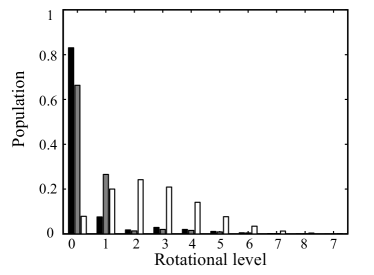
Figure 13: Population in the lowest rotational states of OH${}^{+}\,$(X${}^{3}\Sigma$) after cooling in 10 s using the incoherent radiation from a lamp addressing the $N=1\rightarrow N=2$ and $N=2\rightarrow N=3$ transition (Black columns) and in BBR only (grey columns). The initial 300K Boltzmann distribution is included for comparison (unfilled columns). The spin substructure of the rotational levels is included in the simulation but omitted on the figure.

Appendix A Einstein coefficients

Table 2: Einstein coefficients for selected transitions in s^-1 and corresponding transition frequencies in cm^-1. In the table the quantities have the following meaning: $A^{rot}=A(\nu=0,N=1\rightarrow\nu=0,N=0)$, $A^{vib}=A(\nu=1,N=1\rightarrow\nu=0,N=0)$ for the $\Sigma$-states and $A^{rot}=A(\nu=0,J=\Omega+1\rightarrow\nu=0,J=\Omega)$, $A^{vib}=A(\nu=1,J=\Omega\rightarrow\nu=0,J=\Omega)$ for the $\Pi$-state. A similar notation is used for the transition frequencies. The pure rotational transition rates (first column) indicate the rotational redistribution speed while the vibrational transition rates give the spontaneous decay rate from the excited vibrational state in the pumping schemes. The data largely explains the qualitative difference in cooling efficiency for the molecular ions. Large rotational redistribution rates indicate a fast scheme, while fast spontaneous decays from the excited vibrational state indicate high effective pump rate, i.e. high cooling efficiency. The data for BH${}^{+}\,$is found using the data from Ref. Klein et al. (1982) and the computer programme of Ref. LeRoy (2002) from which the Hönl-London factors were corrected to conform with the multiplet expressions of Sec. IV. Data for OH${}^{+}\,$was found using the same approach and data from Fig. 12. Finally the data on FH${}^{+}\,$was obtained using the data of Refs. Coe et al. (1989); Werner et al. (1984).

	Arot (S-1)	Avib (S-1)	$\omega^{rot}$ (cm-1)	$\omega^{vib}$ (cm-1)
24Mg1H+ (X${}^{1}\Sigma\;$)	$2.5\cdot 10^{-3}$	$20.5$	12.9	1672
11B1H+ (X${}^{2}\Sigma\;$)	$0.2\cdot 10^{-3}$ (Q-branch)	11.5	25.0	2437
	$0.4\cdot 10^{-3}$ (R-branch)	23.0
16O1H+ (X${}^{3}\Sigma\;$)	$3.8\cdot 10^{-3}$ (P-branch)	18.3
	$19.2\cdot 10^{-3}$ (R-branch)	91.6	33.07	2990
	$11.5\cdot 10^{-3}$ (Q-branch)	54.9
	Arot (S-1)	Avib (S-1)	$\omega^{rot}$ (cm-1)	$\omega^{vib}$ (cm-1)
19F1H+ (X${}^{2}\Pi\;$)	$93.8\cdot 10^{-3}$ ($\Omega=\frac{1}{2}$)	82.4	51.6	2964
	$347\cdot 10^{-3}$ ($\Omega=\frac{3}{2}$)	98.9	85.5	2999

Appendix B Hönl-London factors

For completeness we include the details of the derivation of Eqs. (8),(11) and (19).

B.1 ${}^{1}\Sigma\;$ground state

Eq. (4) must be modified if $\Psi_{m}$ and $\Psi_{n}$ are degenerate. The effective Einstein B-coefficient is found as $B_{n,m}=\sum_{\mu}\sum_{\xi}\frac{B_{m_{\xi},n_{\mu}}}{g_{n}}$, where $\mu,\xi$ denote the sub-states of $\Psi_{n}$ and $\Psi_{m}$, respectively, and $g_{n}$ the degeneracy of the initial (upper) state. One summation is done to include transitions to all sub-states of the final state, $m$, while the remaining terms correspond to averaging the result over the sub-states of the initial state. We then define the total transition dipole moment for degenerate states as

$$|\mathcal{D}_{n,m}|^{2}=\sum_{\xi,\mu}|D_{n_{\xi},m_{\mu}}|^{2},$$ (21)

where the summation is done over all transitions between sub-states of the system. The Einstein coefficients between degenerate states then take the form

$$\begin{split}B_{n,m}&=\frac{\pi|\mathcal{D}_{n,m}|^{2}}{3g_{n}\epsilon_{0}\hbar^{2}}\\ A_{n,m}&=\frac{\hbar\omega^{3}}{\pi^{2}c^{3}}B_{n,m},\end{split}$$ (22)

Which is the same as Eq. (4) except for the degeneracy factor. We now move to a molecule-fixed coordinate system. We define the electronic dipole moment function by integrating the dipole operator, $\bm{M}^{mol}$, over the electronic variables, $\tau_{e}$

$$\bm{D}_{e}^{mol}(R)=\int\psi_{e}(\{\bm{r}_{i}^{\prime}\},R)^{\ast}\bm{M}^{mol}\psi_{e}(\{\bm{r}_{i}^{\prime}\},R)d\tau_{e}.$$ (23)

Here we stay in the electronic state defined by the wave function $\psi_{e}(R)$ in the body-fixed frame. We have calculated $\bm{D}_{e}^{mol}(R)$ ab initio with Gaussian Frisch et al. (1995). Details of these calculations are molecule-specific and will be given below.

To transform the dipole moment to the laboratory frame we now specialize to ${}^{1}\Sigma\;$states, postponing the general solution to Sec. IV. For ${}^{1}\Sigma\;$diatomic molecules the cylindrical symmetry of the potential will ensure that $\bm{D}_{e}^{mol}(R)$ points along the internuclear axis. Hence the $Z$-component of $\bm{D}_{e}^{mol}(R)$ in the laboratory system is given by

$$\bm{D}_{e}^{lab}(R)_{Z}=\bm{D}^{mol}_{e}(R)\cdot\hat{Z}=D_{e}^{mol}(R)\cos\theta.$$ (24)

The molecular states are degenerate so it is necessary to sum over all sub-states to obtain the transition dipole moment defined in Eq. (21). In the case of ${}^{1}\Sigma\;$molecules this corresponds to summing over all projections $M_{J}$ of the molecular angular momentum $\bm{J}$. In carrying out the summation over the sub-states in Eq. (21) the selection rule $\Delta M_{J}=0,\pm 1$ makes it possible to rewrite the expression as a single sum over $\mu=M_{J}$ which can be related to the total transition dipole moment. Since the transition probability must be independent of the orientation of the laboratory coordinate system we have

$$|\bm{\mathcal{D}}_{m,n}^{lab}|^{2}=\sum_{M_{J}}|\bm{D}^{lab}|^{2}=3\sum_{M_{J}}|\bm{D}_{Z}^{lab}|^{2}.$$ (25)

Inserting Eq. (24) in Eq. (5) we find

$$\begin{split}\bm{D}^{lab}_{Z}=\int&\psi_{r_{n},\nu_{n}}^{mol}(\theta,\phi,R)^{\ast}D_{e}^{mol}(R)\cos\theta\times\\ &\psi_{r_{m},\nu_{m}}^{mol}(\theta,\phi,R)R^{2}\sin\theta dRd\theta d\phi,\end{split}$$ (26)

where $\psi_{r_{n},\nu_{n}}$ and $\psi_{r_{m},\nu_{m}}$ are the remaining ro-vibrational wave functions obtained after the integration over electronic coordinates in Eq. (23). Now, we assume that the ro-vibrational wave function may be written as a product, $\Psi_{r_{n},\nu_{n}}(R,\theta,\phi)=\Phi_{r_{n}}(\theta,\phi)f_{\nu_{n}}(R)$. Then

$$|\bm{D}_{Z}^{lab}|^{2}=\Big{|}L_{J_{n},M_{n}}^{J_{m},M_{m}}\Big{|}^{2}\times\Big{|}\int f_{\nu_{n}}(R)D_{e}^{mol}(R)f_{\nu_{m}}(R)R^{2}dR\Big{|}^{2},$$ (27)

with

$$L_{J_{n},M_{n}}^{J_{m},M_{m}}=\int{\Phi_{r_{n}}^{lab}}^{\ast}(\theta,\phi)\cos\theta\Phi_{r_{m}}^{lab}(\theta,\phi)\sin\theta d\theta d\phi.$$ (28)

Defining

$$S_{J_{m},J_{n}}=3\sum_{M_{n},M_{m}}\Big{|}L_{J_{n},M_{n}}^{J_{m},M_{m}}\Big{|}^{2}$$ (29)

known as the Hönl-London factors Hönl and London (1925); Kovács (1969); Huber and Herzberg (1979). We combine the above results with Eq. (25) to find the total transition dipole moment entering Eq. (22)

$$|\bm{\mathcal{D}}_{m,n}|^{2}=S_{J_{m},J_{n}}\Big{|}\int f_{\nu_{n}}(R)D_{e}(R)f_{\nu_{m}}(R)R^{2}dR\Big{|}^{2}.$$ (30)

B.2 Hunds case (a)

We use the Hunds case (a) eigenfunctions in the lab frame from Hornkohl and Parigger (1996) (cf. Eq. (10))

$$\begin{gathered}\left\langle{\{\bm{r}_{i}\}\bm{R}|nJM_{J}\Omega S\Sigma}\right\rangle=\\ \sqrt{\frac{2J+1}{8\pi^{2}}}\left\langle{\{\bm{r}_{i}^{\prime}\},R|n}\right\rangle\left\lvert{S\Sigma}\right\rangle\mathcal{D}_{M_{J}\Omega}^{J^{\ast}}(\alpha\beta\gamma),\end{gathered}$$ (31)

and write the lth component of the kth moment transition operator in the laboratory frame, $T_{l}^{k}$, as a similar rotation of the operator working in the molecular rest frame

$$T_{l}^{k}(\{\bm{r}_{i}\}\bm{R})=\sum_{\Lambda=-k}^{k}T_{\Lambda}^{k}(\{\bm{r}_{i}^{\prime}\},R)\mathcal{D}_{l\Lambda}^{k^{\ast}}(\alpha\beta\gamma).$$ (32)

Combining the above equations and performing the integral over Euler angles, while writing the Wigner rotation functions as an expansion over Clebsch-Gordan coefficients Sakurai (1994), one finds the dipole moment transition matrix elements $(k=1)$

$$\begin{gathered}\left\langle{n^{\prime}J^{\prime}M_{J}^{\prime}}\right\rvert T_{l}^{1}(\{\bm{r}_{i}\},\bm{R})\left\lvert{n^{\prime\prime}J^{\prime\prime}M_{J}^{\prime\prime}}\right\rangle=\\ \sqrt{\frac{2J^{\prime\prime}+1}{2J^{\prime}+1}}\sum_{\Lambda=-1}^{1}\left\langle{n^{\prime}\nu^{\prime}}\right\rvert T_{\Lambda}^{1}\left\lvert{n^{\prime\prime}\nu^{\prime\prime}}\right\rangle\\ \left\langle{J^{\prime\prime}M_{J}^{\prime\prime}1l|J^{\prime}M_{J}^{\prime}}\right\rangle\left\langle{J^{\prime\prime}\Omega^{\prime\prime}k\Lambda|J^{\prime}\Omega^{\prime}}\right\rangle.\end{gathered}$$ (33)

Summing over the projections of $\bm{J}$ and emission directions one finds the line strength

$$\begin{split}&\sum_{M_{J}^{\prime},M_{J}^{\prime\prime}}|\left\langle{n^{\prime}J^{\prime}M_{J}^{\prime}}\right\rvert T_{l}^{1}(\{\bm{r}_{i}\}\bm{R})\left\lvert{n^{\prime\prime}J^{\prime\prime}M_{J}^{\prime\prime}}\right\rangle|^{2}=\\ &(2J^{\prime\prime}+1)|\left\langle{n^{\prime}\nu^{\prime}}\right\rvert T_{\Lambda}^{1}\left\lvert{n^{\prime\prime}\nu^{\prime\prime}}\right\rangle|^{2}\times\\ &|\left\langle{J^{\prime\prime}\Omega^{\prime\prime}1(\Omega^{\prime}-\Omega^{\prime\prime})|J^{\prime}\Omega^{\prime}}\right\rangle|^{2}\delta(S^{\prime},S^{\prime\prime})\delta(\Sigma^{\prime},\Sigma^{\prime\prime}).\end{split}$$ (34)

Finally we find the Hönl-London factors in Hunds case (a)

$$\begin{gathered}S(J^{\prime},J^{\prime\prime})=(2J^{\prime\prime}+1)\times\\ |\left\langle{J^{\prime\prime}\Omega^{\prime\prime}1(\Omega^{\prime}-\Omega^{\prime\prime})|J^{\prime}\Omega^{\prime}}\right\rangle|^{2}\delta_{S^{\prime},S^{\prime\prime}}\delta_{\Sigma^{\prime},\Sigma^{\prime\prime}}.\end{gathered}$$ (35)

B.3 Hunds case (b)

We gave the Hunds case (b) eigenfunctions in the laboratory frame in Eq. (18)

$$\begin{gathered}\left\langle{\{\bm{r}_{i}\}\bm{R},nJM_{J}NM_{N}SM_{S}}\right\rangle=\sqrt{\frac{2N+1}{8\pi^{2}}}\times\\ \sum_{M_{S}=-S}^{S}\sum_{M_{N}=-N}^{N}\left\langle{\{\bm{r}_{i}^{\prime}\},R|n}\right\rangle\left\langle{NM_{N}SM_{S}|JM_{J}}\right\rangle\times\\ \left\lvert{SM_{S}}\right\rangle\mathcal{D}_{M_{N}\Lambda}^{N^{\ast}}(\alpha\beta\gamma).\end{gathered}$$ (36)

The rotated dipole moment operator was given in a general form in Eq. (32). We then use the identities Brink and Satchler (1994)

$$\begin{split}\mathcal{D}_{l\lambda}^{k}\mathcal{D}_{m\mu}^{n}=&\sum_{N^{\prime}M^{\prime}\mu^{\prime}}\left\langle{nmkl|N^{\prime}M^{\prime}}\right\rangle\times\\ &\left\langle{n\mu k\lambda|N^{\prime}\mu^{\prime}}\right\rangle\mathcal{D}_{M\mu^{\prime}}^{N^{\prime}}\end{split}$$ (37)

and

$$\int\mathcal{D}_{lm}^{k}\mathcal{D}_{\lambda\mu}^{\kappa}d\Omega=\frac{8\pi^{2}}{2k+1}\delta_{l,\lambda}\delta_{m,\mu}\delta_{k,\kappa},$$ (38)

where $\int d\Omega=\int_{0}^{2\pi}d\alpha\int_{0}^{2\pi}d\gamma\int_{0}^{\pi}d\beta sin\beta$. One thereby finds the expression for the dipole matrix element

$$\begin{gathered}\left\langle{n^{\prime}J^{\prime}M_{J}^{\prime}}\right\rvert T_{l}^{1}(\{\bm{r}_{i}^{\prime}\},\bm{R})\left\lvert{n^{\prime\prime}J^{\prime\prime}M_{J}^{\prime\prime}}\right\rangle=\sqrt{\frac{2N^{\prime\prime}+1}{2N^{\prime}+1}}\left\langle{n^{\prime}\nu^{\prime}}\right\rvert T_{\Lambda^{\prime}-\Lambda^{\prime\prime}}^{1}\left\lvert{n^{\prime\prime}\nu^{\prime\prime}}\right\rangle\left\langle{N^{\prime\prime}\Lambda^{\prime\prime}1(\Lambda^{\prime}-\Lambda^{\prime\prime})|N^{\prime}\Lambda^{\prime}}\right\rangle\times\\ \sum_{\underset{M_{S}^{\prime},M_{S}^{\prime}}{M_{N}^{\prime},M_{N}^{\prime\prime}}}\left\langle{N^{\prime\prime}M_{N}^{\prime\prime}1l|N^{\prime}M_{N}^{\prime}}\right\rangle\left\langle{N^{\prime}M_{N}^{\prime}S^{\prime}M_{S}^{\prime}|J^{\prime}M_{J}^{\prime}}\right\rangle\left\langle{N^{\prime\prime}M_{N}^{\prime\prime}S^{\prime\prime}M_{S}^{\prime\prime}|J^{\prime\prime}M_{J}^{\prime\prime}}\right\rangle\delta_{S^{\prime}S^{\prime\prime}}\delta_{M_{S}^{\prime}M_{S}^{\prime\prime}}.\end{gathered}$$ (39)

This is summed over the projections of $\bm{J}$ and squared to find the dipole transition probability. The task is simplified by rewriting the products of Clebsch-Gordan coefficients in terms of Wigner 6j symbols Sobelman (1992). After some algebra one then finds

$$\begin{gathered}|\left\langle{n^{\prime}J^{\prime}N^{\prime}}\right\rvert T_{l}^{1}\left\lvert{n^{\prime\prime}J^{\prime\prime}N^{\prime\prime}}\right\rangle|^{2}=\frac{1}{3}(2N^{\prime\prime}+1)\times\\ (2J^{\prime}+1)(2J^{\prime\prime}+1)\left\langle{n^{\prime}\nu^{\prime}}\right\rvert T_{\Lambda^{\prime}-\Lambda^{\prime\prime}}^{1}\left\lvert{n^{\prime\prime}\nu^{\prime\prime}}\right\rangle^{2}\times\\ \left\langle{N^{\prime\prime}\Lambda^{\prime\prime}1(\Lambda^{\prime}-\lambda^{\prime\prime})|N^{\prime}\Lambda^{\prime}}\right\rangle^{2}\begin{Bmatrix}S&N^{\prime\prime}&J^{\prime\prime}\\ 1&J^{\prime}&N^{\prime}\end{Bmatrix}^{2}.\end{gathered}$$ (40)

Summing over the emission directions cancels the factor of $\frac{1}{3}$, leaving the expression for the H nl-London factor in Hunds case (b)

$$\begin{gathered}S(J^{\prime},J^{\prime\prime})=(2N^{\prime\prime}+1)(2J^{\prime}+1)\times\\ (2J^{\prime\prime}+1)\left\langle{N^{\prime\prime}\Lambda^{\prime\prime}1(\Lambda^{\prime}-\Lambda^{\prime\prime})|N^{\prime}\Lambda^{\prime}}\right\rangle^{2}\times\\ \begin{Bmatrix}S&N^{\prime\prime}&J^{\prime\prime}\\ 1&J^{\prime}&N^{\prime}\end{Bmatrix}^{2}\delta_{S^{\prime}S^{\prime\prime}}.\end{gathered}$$ (41)

References

- Jochim et al. (2003) S. Jochim, M. Bartenstein, A. A. G. H. S. Riedl, C. Chin, J. H. Denschlag, and R. Grimm, Science 302, 2101 (2003).
- Zwierlein et al. (2003) M. W. Zwierlein, C. A. Stan, C. H. Schunck, S. M. F. Raupach, S. Gupta, Z. Hadzibabic, and W. Ketterle, Phys. Rev. Lett. 91, 250401 (2003).
- Greiner et al. (2003) M. Greiner, C. A. Regal, and D. S. Jin, Nature 426, 537 (2003).
- Bethlem et al. (2002) H. Bethlem, F. Crompvoets, R. Jongma, S. van de Meerakker, and G. Meijer, Phys. Rev. A 65, 053416 (2002).
- van de Meerakker et al. (2001) S. Y. van de Meerakker, R. T. Jongma, H. L. Bethlem, and G. Meijer, Phys. Rev. A 64, 041401 (2001).
- Crompvoets et al. (2002) F. M. Crompvoets, R. T. Jongma, H. L. Bethlem, A. J. van Roij, and G. Meijer, Phys. Rev. Lett. 89, 093004 (2002).
- Bethlem and Meijer (2003) H. Bethlem and G. Meijer, Int. Rev. Phys. Chem. 22, 73 (2003).
- Weinstein et al. (1998) J. D. Weinstein, R. deCarvalho, T. Guillet, B. Friedrich, and J. M. Doyle, Nature 395, 148 (1998).
- Egorov et al. (2002) D. Egorov, T. Lahaye, W. Sch llkopf, B. Friedrich, and J. M. Doyle, Phys. Rev. A 66, 043401 (2002).
- van de Meerakker et al. (2003) S. Y. T. van de Meerakker, B. G. Sartakov, A. P. Mosk, R. T. Jongma, and G. Meijer, Phys. Rev. A 68, 032508 (2003).
- Snow (1992) T. P. Snow, in Interstellar Molecules, edited by B. H. Andrew (Reidel, Dordrecht, 1992), vol. 87 of Proceedings of the IAU Symposium, p. 247.
- Snyder (1992) L. E. Snyder, in Astrochemistry of Cosmic Phenomena, edited by P. D. Singh (Kluwer Academic, Dordrecht, 1992), vol. 150 of Proceedings of the IAU symposium, p. 427.
- Wegmann et al. (1999) R. Wegmann, K. Jockers, and T. Bonev, Planet. Space Sci. 47, 745 (1999).
- Demille (2002) D. Demille, Phys. Rev. Lett. 88, 067901 (2002).
- Tesch and de Vivie-Riedle (2002) C. M. Tesch and R. de Vivie-Riedle, Phys. Rev. Lett. 89, 157901 (2002).
- Mølhave and Drewsen (2000) K. Mølhave and M. Drewsen, Phys. Rev. A 62, 011401(R) (2000).
- Drewsen et al. (2003) M. Drewsen, I. Jensen, J. Lindballe, N. Nissen, R. Martinussen, A. Mortensen, P. Staanum, and D. Voigt, Int. J. Mass Spectrom. 229, 83 (2003).
- Schiller and L mmerzahl (2003) S. Schiller and C. L mmerzahl, Phys. Rev. A 68, 053406(5) (2003).
- (19) U. Fr hlich, B. Roth, P. Antonini, C. L mmerzahl, A. Wicht, and S. Schiller, to appear in: Proceedings of the WE-Heraeus Seminar on Astrophysics, Clocks and Fundamental Constants (2004).
- van Eijkelenborg et al. (1999) M. A. van Eijkelenborg, M. E. M. Storkey, D. M. Segal, and R. C. Thompson, Phys. Rev. A 60, 3903 (1999).
- Vogelius et al. (2002) I. S. Vogelius, L. B. Madsen, and M. Drewsen, Phys. Rev. Lett. 89, 173003 (2002).
- Vogelius et al. (2004) I. S. Vogelius, L. B. Madsen, and M. Drewsen, physics/0406082 (2004).
- Schutte (2001) C. J. H. Schutte, Chem. Phys. Lett. 350, 181 (2001).
- Huber and Herzberg (1979) K. Huber and G. Herzberg, Molecular Spectra and Molecular Structure (Van Nostrand Reinhold Company, 1979).
- Loudon (1983) R. Loudon, The quantum theory of light (Clarendon Press, Oxford, 1983).
- Tatum (1966) J. B. Tatum, Can. Journ. Phys 44, 2944 (1966).
- Kovács (1969) I. Kovács, Rotational Structure in the Spectra of Diatomic Molecules (Adam Hilger Ltd, London, 1969), ISBN 85274.142.1.
- Whiting et al. (73) E. E. Whiting, J. A. Paterson, I. Kovacs, and R. W. Nicholls, J. Mol. Spec. 47, 84 (73).
- Frisch et al. (1995) M. Frisch et al., Tech. Rep., Gaussian inc., Pittsburgh, PA (1995).
- LeRoy (2002) R. J. LeRoy, Level 7.5: A Computer Program for Solving the Radial Schrödinger Equation for Bound and Quasibound Levels (2002), the source code and manual for this program may be obtained from the ”Computer Programs” link on the www site http://leroy.uwaterloo.ca.
- Foresman and Frisch (1996) J. B. Foresman and Æ. Frisch, Exploring Chemistry with Electronic Structure Methods (Gaussian, Inc., Pittsburgh, PA, 1996), and references therein.
- Møller and Plesset (1934) C. Møller and M. S. Plesset, Phys. Rev. 46, 618 (1934).
- Bauschlicher and Langhoff (1991) C. W. Bauschlicher and S. R. Langhoff, Chem. Rev. 91, 701 (1991).
- Lawley (1987) K. P. Lawley, ed., Advances in Chemical Physics: Ab initio methods in quantum chemistry, vol. 67 and 69 (Wiley, New York, 1987).
- Krishnan and Pople (1978) R. Krishnan and J. A. Pople, Int. J. Quant. Chem. 14, 91 (1978).
- Pople et al. (1987) J. A. Pople, M. Head-Gordon, and K. Raghavachari, J. Chem. Phys. 87, 5968 (1987).
- Zemke et al. (1984) W. Zemke, R. E. Olson, K. K. Verma, W. C. Stwalley, and L. B, J. Chem. Phys. 80, 356 (1984).
- Ornellas et al. (1983) F. R. Ornellas, W. C. Stwalley, and W. T. Zemke, J. Chem. Phys. 79, 5311 (1983).
- Machado and Ornellas (1991) F. B. C. Machado and F. R. Ornellas, J. Chem. Phys. 94, 7237 (1991).
- Dormand and Prince (1980) J. R. Dormand and P. J. Prince, J. Comp. Appl. Math. 6, 19 (1980).
- Kimmitt (1970) M. F. Kimmitt, Far-Infrared Techniques (Pion Limited, 1970).
- Hornkohl and Parigger (1996) J. O. Hornkohl and C. Parigger, Am. J. Phys. 64, 623 (1996).
- Brink and Satchler (1994) D. Brink and G. Satchler, Angular Momentum (Clarendon Press, Oxford, 1994), ISBN 0-19-851759-9.
- Coe et al. (1989) J. V. Coe, J. C. Owrutsky, E. R. Keim, N. V. Agman, D. C. Hovde, and R. J. Saykally, J. Chem. Phys 90, 3893 (1989).
- Werner et al. (1984) H.-J. Werner, P. Rosmus, W. Sch tzl, and W. Meyer, J. Chem. Phys. 80, 831 (1984).
- Lefebvre-Brion and Field (1986) H. Lefebvre-Brion and R. W. Field, Perturbations in the Spectra of Diatomic Molecules (Academic Press Inc., Orlando, 1986), ISBN 0-12-442691-3.
- Klein et al. (1982) R. Klein, P. Rosmus, and H. J. Werner, J. Chem. Phys. 77, 3559 (1982).
- Werner et al. (1983) H. J. Werner, P. Rosmus, and E. A. Reinsch, J. Chem. Phys 79, 905 (1983).
- Larsson et al. (1989) M. Larsson, J. B. A. Mitchell, and I. F. Schneider, eds., Dissociative recombination: theory, experiment and applications IV (World Scientific, Stockholm, 1989), ISBN 981-02-4077-5.
- Hönl and London (1925) H. Hönl and F. London, Z. Physik 33, 803 (1925).
- Sakurai (1994) J. J. Sakurai, Modern Quantum Mechanics (Addison-Wesley, 1994).
- Sobelman (1992) I. I. Sobelman, Atomic Spectra and Radiative Transitions (Springer, 1992), 2nd ed.