Electrochemical thin films at and above the classical limiting current

Abstract

We study a model electrochemical thin film at dc currents exceeding the classical diffusion-limited value. The mathematical problem involves the steady Poisson-Nernst-Planck equations for a binary electrolyte with nonlinear boundary conditions for reaction kinetics and Stern-layer capacitance, as well as an integral constraint on the number of anions. At the limiting current, we find a nested boundary layer structure at the cathode, which is required by the reaction boundary condition. Above the limiting current, a depletion of anions generally characterizes the cathode side of the cell. In this regime, we derive leading-order asymptotic approximations for the (i) classical bulk space-charge layer and (ii) another, nested highly charged boundary layer at the cathode. The former involves an exact solution to the Nernst-Planck equations for a single, unscreened ionic species, which may apply more generally to Faradaic conduction through very thin insulating films. By matching expansions, we derive current-voltage relations well into the space-charge regime. Throughout our analysis, we emphasize the strong influence of the Stern-layer capacitance on cell behavior.

Introduction

Thin-film technologies offer a promising way to construct
rechargeable micro-batteries, which can be directly integrated into modern electronic circuits [1, 2, 3, 4, 5, 6]. Due to the power-density requirements of many applications, such as portable electronics, micro-batteries are likely to be operated under at high current density, possibly exceeding diffusion limitation. In a thin film, very large electric fields are easily produced by applying only small voltages, due to the small electrode separation, which may be comparable to the Debye screening length. Under such conditions, the traditional postulates of macroscopic electrochemical systems [7, 8] — bulk electroneutrality and equilibrium double layers — break down near the classical diffusion-limited current [9]. The mathematical justification for these postulates is based on matched asymptotic expansions in the limit of thin double layers [12, 13, 14], which require subtle modifications at large currents.

The concept of a “limiting current”, due to the maximum, steady-state flux of diffusion across an electrochemical cell, was introduced by Nernst a century ago [10], but it was eventually realized that the classical theory is flawed, as illustrated in Figure 1 by numerical solutions to our model problem below. Levich was perhaps the first to notice that the assumption of bulk electroneutrality yields approximate solutions to the Poisson-Nernst-Planck (PNP) equations, which are not self consistent near the limiting current, since the predicted charge density eventually exceeds the salt concentration near the cathode [11]. This paradox was first resolved by Smyrl and Newman, who showed that the double layer expands at the limiting current, as the Poisson-Boltzmann approximation of thermal equilibrium breaks down [15]. Rubinstein and Shtilman later pointed out that mathematical solutions also exist for larger currents, well above the classical limiting value, characterized by a region of non-equilibrium “space charge” extending significantly into the neutral bulk [16].

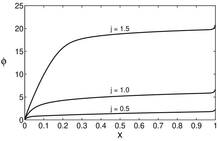
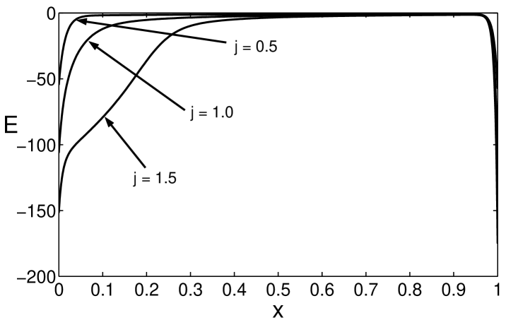
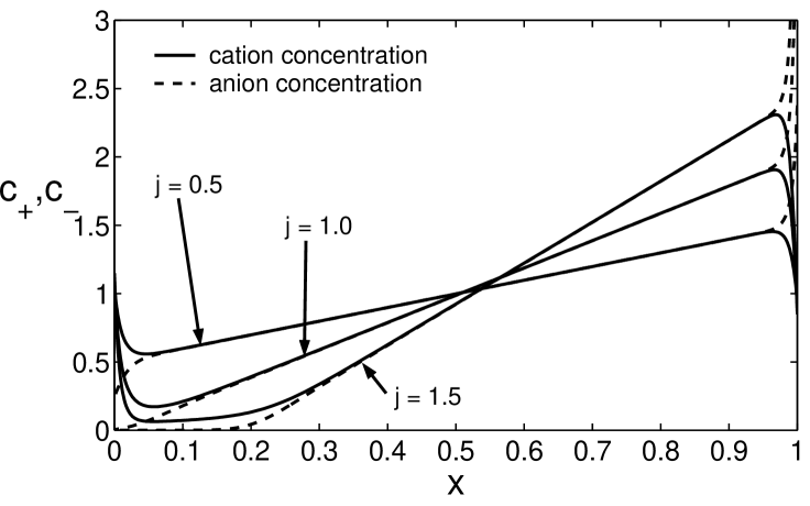
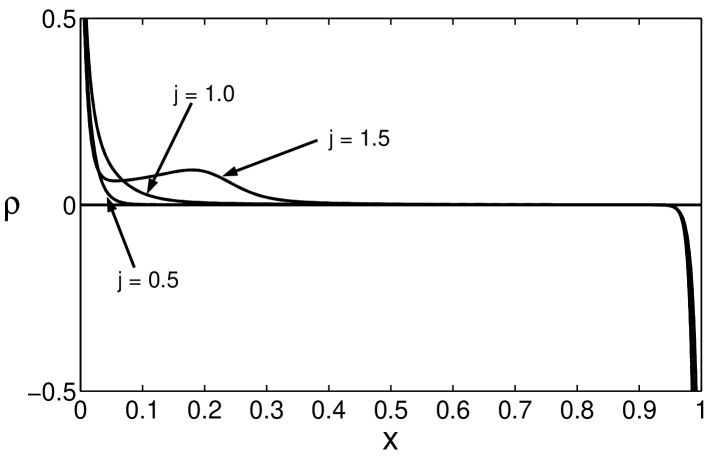
Fig. 1: Profiles of the dimensionless potential (top left), electric field (top right), total ionic concentration (bottom left), and charge density (bottom right) in three regimes: below the classical diffusion-limited current ($j=0.5$), at the limiting current ($j=1$), and above the limiting current ($j=1.5$). These are numerical solutions to our model problem with the following dimensionelss parameters: $\epsilon=0.01$, $\delta=0$, $k_{c}=10$, $j_{r}=10$.

The possiblity of superlimiting currents has been studied extensively in the different context of bulk liquid electrolytes, where a thin space-charge layer drives nonlinear electro-osmotic slip. This phenomenon of “electro-osmosis of the second kind” was introduced by Dukhin for the nonlinear electrophoresis of ion-selective, conducting colloidal particles [17], and Ben and Chang have recently studied it in microfluidics [18]. The mathematical analysis of second-kind electro-osmosis using matched asymptotic expansions, similar to the approach taken here, was first developed by Rubinstein and Zaltzman for related phenomena at electrodialysis membranes [19, 20]. In earlier studies, the space-charge layer was also invoked by Bruinsma and Alexander [21] to predict hydrodynamic instability during electrodeposition and by Chazalviel [22] in a controversial theory of fractal electrochemical growth.

As in our companion paper on sublimiting currents [9], here we consider (typically solid or gel) thin films, e.g. arising in micro-batteries, which approach the classical limiting current without hydrodynamic instability. At micron or smaller length scales, the space charge layer need not be “thin” compared to the film thickness, so we also analyze currents well above the classical limiting current, apparently for the first time. In both regimes, close to and far above the classical limiting current, we derive matched asymptotic expansions for the concentration profiles and potential, which we compare against numerical solutions. In addition to our focus on superlimiting currents and small systems, a notable difference with the literature on second-kind electro-osmosis is our use of nonlinear boundary conditions for Faradaic electron-transfer reactions, assuming Butler-Volmer kinetics and a compact Stern layer. We also analyze the current-voltage relation, thus extending our analogous results for thin films below the limiting current [9].

1 Statement of Problem

Before delving into the analysis (and to make this paper as self-contained as possible), we review governing equations and boundary conditions. We shall focus solely on the dimensionless formulation of the problem. For details of the physical assumptions underlying the mathematical model, the reader is referred to Ref. [9].

The transport of cations and anions is described by the steady Nernst-Planck equations

$$\frac{d^{2}c_{+}}{dx^{2}}+\frac{d}{dx}\left(c_{+}\frac{d\phi}{dx}\right) = 0$$ (1)

$$\frac{d^{2}c_{-}}{dx^{2}}-\frac{d}{dx}\left(c_{-}\frac{d\phi}{dx}\right) = 0.$$ (2)

while Poisson’s equation relates the electric potential to the charge density,

$$-\epsilon^{2}\frac{d^{2}\phi}{dx^{2}}=\frac{1}{2}(c_{+}-c_{-}).$$ (3)

Here $\epsilon$ is a small dimensionless parameter equal to the ratio of the Debye screening length to the electrode separation (or film thickness). Note that this formulation assumes constant material properties, such as diffusivity, mobility, and dielectric coefficient, and neglects any variations which may occur at large electric fields. The factor of $1/2$ multiplying the charge density $c_{+}-c_{-}$ is present merely for convenience. The domain for the system of eqns. (1)-(3) is $0<x<1$.

The two Nernst-Planck equations are easily integrated under the physical constraint that the boundaries are impermeable to anions (i.e. zero flux of anions at $x=0$) and taking the nondimensional current density at the electrodes to be $4j$:

$$\frac{dc_{+}}{dx}+c_{+}\frac{d\phi}{dx} = 4j$$ (4)

$$\frac{dc_{-}}{dx}-c_{-}\frac{d\phi}{dx} = 0.$$ (5)

Then by introducing the average ion concentration and (half) the charge density

$$c=\frac{1}{2}(c_{+}+c_{-})\ \ \ \textrm{and}\ \ \ \rho=\frac{1}{2}(c_{+}-c_{-}),$$ (6)

we can derive a more symmetric form for the coupled Poisson-Nernst-Planck equations:

$$\frac{dc}{dx}+\rho\frac{d\phi}{dx}=2j$$ (7)

$$\frac{d\rho}{dx}+c\frac{d\phi}{dx}=2j$$ (8)

$$-\epsilon^{2}\frac{d^{2}\phi}{dx^{2}}=\rho.$$ (9)

For this system of one second-order and two first-order differential equations, we require four boundary conditions and one integral constraint:

$$\phi(0)-\delta\epsilon\frac{d\phi}{dx}(0) = 0,$$ (10)

$$\phi(1)+\delta\epsilon\frac{d\phi}{dx}(1) = v,$$ (11)

$$k_{c}[c(0)+\rho(0)]e^{\alpha_{c}\phi(0)}-j_{r}e^{-\alpha_{a}\phi(0)} = j,$$ (12)

$$-k_{c}[c(1)+\rho(1)]e^{\alpha_{c}(\phi(1)-v)}+j_{r}e^{-\alpha_{a}(\phi(1)-v)} = j,$$ (13)

$$\int_{0}^{1}[c(x)-\rho(x)]dx = 1,$$ (14)

The first two boundary conditions, Eqs. (10)–(11), account for the intrinsic capacitance of the compact part of the electrode-electrolyte interface, as originally envisioned by Stern. In these boundary conditions, $\delta$ is a dimensionless parameter which is a measure of the strength of the surface capacitance, and $v$ is the total voltage drop across the cell.

The next two boundary conditions, Eqs. (12)–(13), are Butler-Volmer rate equations which represent the kinetics of Faradaic electron-transfer reactions at each electrode, with an Arhhenius dependence on the compact layer voltage. In these equations, $k_{c}$ and $j_{r}$ are dimensionless reaction rate constants and $\alpha_{c}$ and $\alpha_{a}$ are transfer coefficients for the electrode reaction. It is worth noting that $\alpha_{c}$ and $\alpha_{a}$ do not vary too much from system to system; typically they have values between $0$ and $1$ and often both take on values near $1/2$.

Finally, the integral constraint, Eq. (14), reflects the fact that the total number of anions is fixed, assuming that anions are not allowed to leave the electrolyte by Faradaic processes or specific adsorption. It is important to understand that the need for an extra boundary condition/constraint reflects that the current-voltage relationship, $j(v)$, or “polarographic curve”, is not given a priori. As usual in one-dimensional problems [9], it is easier to assume galvanostatic forcing at fixed curent, $j$, and then solve for the cell voltage, $v(j)$, by applying the boundary condition (11), rather than the more common case of potentiostatic forcing at fixed voltage, $v$. For this reason, we take the former approach in our analysis. For steady-state problems, the two kinds of forcing are equivalent and yield the same (invertible) polaragraphic curve, $j(v)$ or $v(j)$.

For some of our analysis, it will be convenient to further simplify the problem by introducing the dimensionless electric field, $E\equiv-\frac{d\phi}{dx}$. This transformation is useful because three of the five independent constraints can be expressed in terms of these variables, without explicit dependence on $\phi(x)$, namely the two Butler-Volmer rate equations,

$$k_{c}(c(0)+\rho(0))e^{-\alpha_{c}\delta\epsilon E(0)}-j_{r}e^{\alpha_{a}\delta\epsilon E(0)} = j,$$ (15)

$$-k_{c}(c(1)+\rho(1))e^{\alpha_{c}\delta\epsilon E(1)}+j_{r}e^{-\alpha_{a}\delta\epsilon E(1)} = j,$$ (16)

and the integral constaint on the total number of anions, Eq. (14). The potential is recovered by integrating the electric field and applying the Stern boundary conditions Eqs. (10) and (11).

2 Unified Analysis at All Currents

2.1 Master Equation for the Electrostatic Potential

We begin our analysis by reducing the governing equations, Eqs. (7) through (9), to a single master equation for the electrostatic potential. Substituting Eq. (9) into Eq. (7) and integrating, we obtain an expression for the average concentration

$$c(x)=\b{c}_{o}+2jx+\frac{\epsilon^{2}}{2}\left(\frac{d\phi}{dx}\right)^{2}.$$ (17)

Then by applying the integral constraint, Eq. (14), we find that the integration constant, $\b{c}_{o}$ , is given by

$$\b{c}_{o}=(1-j)-\epsilon^{2}\left[\left(\left.\frac{d\phi}{dx}\right)\right|_{x=1}-\left(\left.\frac{d\phi}{dx}\right)\right|_{x=0}+\frac{1}{2}\int_{0}^{1}\left(\frac{d\phi}{dx}\right)^{2}dx\right]$$ (18)

Note that when the electric field is $O(1)$, Eqns. (17) and (18) reduce to the leading-order concentration in the bulk when $j$ is sufficiently below the limiting current [9]. We can now eliminate $\rho$ and $c$ from Eq. (8) to arrive at a single master equation for $\phi$

$$\epsilon^{2}\left[-\frac{d^{3}\phi}{dx^{3}}+\frac{1}{2}\left(\frac{d\phi}{dx}\right)^{3}\right]+\left(\b{c}_{o}+2jx\right)\frac{d\phi}{dx}=2j,$$ (19)

or equivalently for the electric field $E$

$$\epsilon^{2}\left[\frac{d^{2}E}{dx^{2}}-\frac{1}{2}E^{3}\right]-\left(\b{c}_{o}+2jx\right)E=2j.$$ (20)

Once this equation is solved, the concentration, $c$, and charge density, $\rho$, are computed using Eq. (17) and Poisson’s equation, Eq. (9).

The master equation has been derived in various equilivalent forms since the 1960s. Grafov and Chernenko [24] first combined Eqs. (4), (5) and (9) to obtain a single nonlinear differential equation for the anion concentration, $c_{-}$, whose general solution they expressed in terms of Painlevé’s transcendents. The master equation for the electric field, Eq. (20), was first derived Smyrl and Newman [15], in the special case of the classical limiting current, where $j=1$ and $\b{c}_{o}=0$, where they discovered a non-equilibrium double layer of width, $\epsilon^{2/3}$, which is apparent from the form of the master equation. We shall study the general electric-field and potential equations for an arbitrary current, $j$, focusing on boundary-layer structure in the limiting and superlimiting regimes.

2.2 Efficient Numerical Solution

To solve the master equation for the electric field with the boundary conditions and integral constraint, we use the Newton-Kantorovich method [25]. Specifically, we use a Chebyshev pseudospectral discretization to solve the linearized boundary-value problem at each iteration [25, 26]. Our decision to use this method is motivated by its natural ability to resolve boundary layers and its efficient use of grid points. We are able to get accurate results for many parameter regimes very quickly (typically less than a few minutes on a workstation) with only a few hundred grid points, which would not be possible at large currents and/or thin double layers using a naive finite-difference scheme. It is important to stress that the boundary conditions and the integral constraint are explicitly included as part of the Newton-Kantorovich iteration. Therefore, the linear BVP solved in each iteration is actually an integro-differential differential equation with boundary conditions that are integro-algebraic equations.

To ensure convergence at high currents, we use continuation in the current density parameter, $j$, and start with a sufficiently low initial $j$ that the bulk electroneutral solution is an acceptable initial guess; often, initial $j$ values relatively high compared to the diffusion-limited current are acceptable. Continuation in the $\delta$ parameter is also sometimes necessary to compute solutions at high $\delta$ values.

The results of the numerical method are presented in the figures below and in Ref. [9] to test our analytical approximations obtained by asymptotic analysis.

2.3 Recovery of Classical Results Below the Limiting Current, $j\ll 1-\epsilon^{2/3}$

In the low-current regime, the master equation admits the two distinguished limits around $x=0$ that arise in the classical analysis: $x=O(1)$ and $x=O(\epsilon)$. When $x=O(1)$, we find the usual bulk electric field from Eq. (19) and the bulk concentration from Eq. (17). When $x=O(\epsilon)$, the master equation can be rescaled using $x=\epsilon y$ to obtain

$$-\frac{d^{3}\phi}{dy^{3}}+\frac{1}{2}\left(\frac{d\phi}{dy}\right)^{3}+\b{c}_{o}\frac{d\phi}{dy}+2jy\epsilon\frac{d\phi}{dy}=2j\epsilon$$ (21)

which is equivalent to the classical theory at leading order [9]. In particular, the Gouy-Chapman structure of the double-layer can be derived directly from the Smyrl-Newman equation in this limit [23].

The anode boundary layer comes from a similar $O(\epsilon)$ scaling around $x=1$. Note that in the $j\ll 1-\epsilon^{2/3}$ regime, the scaling $x=O(\epsilon^{2/3})$ is not a distinguished limit because the $\b{c}_{o}\left(\frac{d\phi}{dx}\right)$ term would dominate all other terms in Eq. (19).

3 Nested Boundary Layers at the Limiting Current, $j=1-O(\epsilon^{2/3})$

In this section, we show that a nontrivial nested boundary-layer structure emerges at the classical limiting current when general boundary conditions are considered.

3.1 Expansion of the Double Layer Out of Equilibrium

As discussed in the companion paper [9], the classical analysis breaks down as the current approaches the diffusion-limited current. Mathematically, the breakdown occurs because a new distinguished limit for the master equation appears as $j\rightarrow 1$. Rescaling the master equation using $x=\epsilon^{2/3}z$ gives us

$$-\frac{d^{3}\phi}{dz^{3}}+\frac{1}{2}\left(\frac{d\phi}{dz}\right)^{3}+\frac{\b{c}_{o}}{\epsilon^{2/3}}\frac{d\phi}{dz}+2jz\frac{d\phi}{dz}=2j,$$ (22)

which implies that we have a meaningful distinguished limit if $\b{c}_{o}=O(\epsilon^{2/3})$ or, equivalently, $j=1-O(\epsilon^{2/3})$. As first noticed by Smyrl and Newman [15], the appearance of the $\epsilon^{2/3}$ scaling corresponds to the expansion of the diffuse charge layer that arises at the classical limiting current (see Figure 2). In this regime, the double layer is no longer in Poisson-Boltzmann equilibrium at leading order.

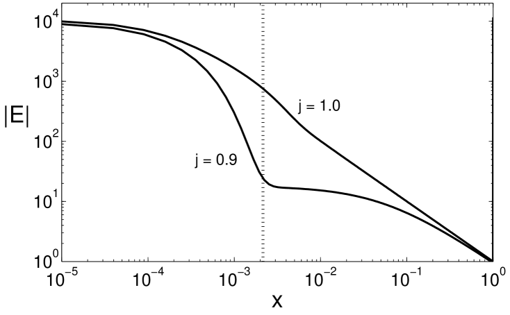
Fig. 2: Numerical solutions for the dimensionless electric field $E(x)$ at current densities of $j=0.9$ and $j=1.0$ demonstrating the expansion of the diffuse layer at the limiting current ($k_{c}=1$, $j_{r}=2$, $\delta=0.1$ and $\epsilon=0.0001$). For reference, the vertical line shows where $x=\epsilon^{2/3}$.

Unfortunately, at this scale, all terms in Eq. (22) are $O(1)$, so we are forced to solve the full equation. Although general solutions can be expressed in terms of Painlevé’s transcendents [8, 18, 24], these are not convenient for applying our nonlinear boundary conditions or obtaining physical insight. Even when $\b{c}_{o}=o(\epsilon^{2/3})$, we are left with a complicated differential equation which does not admit a simple analytical solution. However, in the case $\b{c}_{o}=o(\epsilon^{2/3})$, it is possible to study the asymptotic behavior of the solution in the limits $z\rightarrow 0$ and $z\rightarrow\infty$ by considering the behavior of the neighboring asymptotic layers.

3.2 Nested Boundary Layers when $|1-j|=o(\epsilon^{2/3})$

The appearance of the new distinguished limit for $j=1-O(\epsilon^{2/3})$ does not destroy the ones that exist in the classical analysis. In particular, the $O(\epsilon)$ boundary layer at $x=0$ does not vanish. This inner layer was overlooked by Smyrl and Newman because they assumed a fixed surface charge density given by the equilibrium zeta potential [15], rather than more realistic boundary conditions allowing for surface-charge variations.

In the general case, a set of nested boundary layers exists when the current is near the classical limiting current. For convenience, we shall refer to the $x=O(\epsilon^{2/3})$ and the $x=O(\epsilon)$ regions as the “Smyrl-Newman” and “inner diffuse” layers, respectively. It is important to realize that without the $O(\epsilon)$ layer, it would be impossible, in general, to satisfy the boundary conditions of the original problem. To see this, consider the reaction boundary condition at $x=0$, Eq. (12). To estimate the $c$ and $\rho$ at the electrode surface, we rescale Eq. (17) and Poisson’s equation using $x=\epsilon^{2/3}z$ to obtain

$$c = \@text@baccent{c}_{o}+2j\epsilon^{2/3}z+\frac{\epsilon^{2/3}}{2}\left(\frac{d\phi}{dz}\right)^{2}$$ (23)

$$\rho = -\epsilon^{2/3}\frac{d^{2}\phi}{dz^{2}},$$ (24)

which means that the concentration and charge density are both $O(\epsilon^{2/3})$ since $\b{c}_{o}=o(\epsilon^{2/3})$ when $|1-j|=o(\epsilon^{2/3})$. Then, from the Stern boundary condition, we have $\phi(0)=-\delta\epsilon{\bar{E}}=-\delta\epsilon^{1/3}{\grave{E}}=O(\delta\epsilon^{1/3})$. Plugging these estimates into the reaction boundary condition, we find

$$k_{c}O(\epsilon^{2/3})e^{\alpha_{c}\delta\epsilon^{1/3}{\grave{E}}(0)}=j+j_{r}e^{-\alpha_{a}\delta\epsilon^{1/3}{\grave{E}}(0)}=O(1).$$ (25)

For this equation to be satisfied, $\delta$ is constrained to be huge for $\epsilon$ near $0$: $\delta=O\left(\left|\log\epsilon^{2/3}\right|/\epsilon^{1/3}\right)\gg 1$. But $\delta$ is an independently assigned physical parameter, so there is no reason that it should have to satisfy this constraint. Thus, we are lead to the conclusion that there must be a nested inner boundary layer in order to satisfy the Butler-Volmer boundary condition when $\delta$ is small compared to $\left|\log\epsilon^{2/3}\right|/\epsilon^{1/3}$. In other words, for insufficiently large $\delta$, the reaction boundary condition requires that the cation concentration is $O(1)$ at $x=0$, which implies the existence of a boundary layer between the Smyrl-Newman layer and the boundary. As can be seen in figure 3, the cathode layer concentration decreases significantly as $\delta$ is increased.

To analyze Eq. (22), it is convenient to focus on the electric field rather than the potential. In terms of the scaled electric field, ${\grave{E}}(z)\equiv-\frac{d\phi}{dz}=\epsilon^{2/3}E(x)$, Eq. (22) becomes

$$\frac{d^{2}{\grave{E}}}{dz^{2}}-\frac{1}{2}{\grave{E}}^{3}-2j\left(z{\grave{E}}+1\right)=\frac{\b{c}_{o}}{\epsilon^{2/3}}{\grave{E}}$$ (26)

which we shall refer to as the “Smyrl-Newman equation”. From Eq. (71) in Ref. [9], we know that the first few terms in the expansion for the bulk electric field at the limiting current are

$$-{\bar{E}}(x) = \frac{1}{x}+\frac{3\epsilon^{2}}{4x^{4}}+\frac{111\epsilon^{4}}{16x^{7}}+\frac{6045\epsilon^{6}}{32x^{10}}+\ldots$$ (27)

$$= \frac{1}{\epsilon^{2/3}}\left(\frac{1}{z}+\frac{3}{4z^{4}}+\frac{111}{16z^{7}}+\frac{6045}{32z^{10}}+\ldots\right).$$

Since the second series is asymptotic for $z\gg 1$, the expansion in the bulk is valid for $x\gg\epsilon^{2/3}$. In order to match the solution in the Smyrl-Newman layer to the bulk, we expect the asymptotic solution to Eq. (26) as $z\rightarrow\infty$ to be given by the expression in parentheses in Eq. (27). We could also have arrived at this result by directly substituting an asymptotic expansion in $1/z$ and matching coefficients. As we can see in Figure 3 the leading order term in Eq.(27) is a good approximation to the exact solution in the bulk and is matched by the solution in the Smyrl-Newman layer as it extends into the bulk.

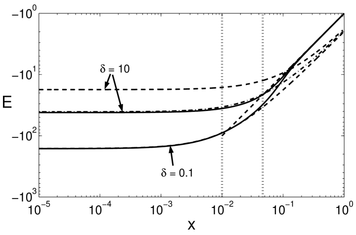
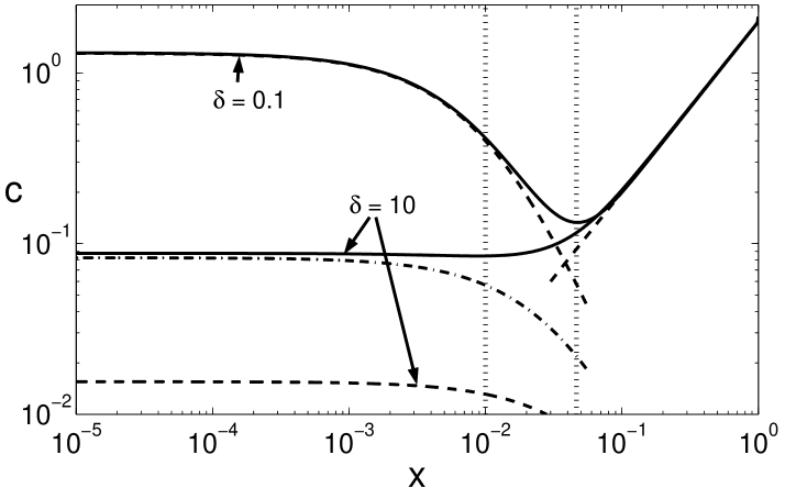
Fig. 3: Numerical solutions (solid lines) for the dimensionless electric field $E(x)$ and concentration $c(x)$ at the classical diffusion-limited current ($j=1$) compared with leading order asymptotic approximations (dashed and dot-dashed lines) for $k_{c}=1$, $j_{r}=2$, $\epsilon=0.01$ and $\delta=0.1,10$. The leading order bulk approximations for $E(x)$ and $c(x)$ are given by Eq. (27) and $c(x)=2jx$, respectively. In the diffuse layer, the leading order approximations are given by Eqs. (29) and (30). For the $\delta=10$ curves, the difference between the dashed and dot-dashed curves is that the dahsed curve uses an approximate value for $B$ given by Eq. (35) while the dot-dashed curve uses a $B$ value calculated by numerically solving Eq. (32). For reference, the vertical lines show where $x=\epsilon$ and $x=\epsilon^{2/3}$. The thin anode diffuse layer field is not shown.

We now turn our attention towards the “inner diffuse” layer which gives us the asymptotic behavior of the Smyrl-Newman equation in the limit $z\rightarrow 0$. Introducing the scaled variables $y=x/\epsilon=z/\epsilon^{1/3}$ and ${\breve{E}}=\epsilon{\bar{E}}=\epsilon^{1/3}{\grave{E}}$, Eq. (26) becomes

$$\frac{d^{2}{\breve{E}}}{dy^{2}}-\frac{1}{2}{\breve{E}}^{3}-2j\epsilon\left(y{\breve{E}}+1\right)=\b{c}_{o}{\breve{E}}.$$ (28)

Near the limiting current (i.e. $\b{c}_{o}=O(\epsilon^{2/3})$), ${\breve{E}}$ satisfies $\frac{d^{2}{\breve{E}}}{dy^{2}}=\frac{1}{2}{\breve{E}}^{3}$ at leading order with the boundary condition ${\breve{E}}\rightarrow 0$ as $y\rightarrow\infty$ from the matching condition that ${\grave{E}}$ remains bounded as $z\rightarrow 0$. Integrating this equation twice with the observation that $\frac{d{\breve{E}}}{dy}>0$ gives us

$${\breve{E}}(y)\sim-\frac{2}{y+b}$$ (29)

where $b$ is a constant determined by applying the Butler-Volmer reaction boundary condition at the cathode. We can estimate $\breve{c}(y)$ and ${\breve{\rho}}(y)$ by substituing Eq. (29) into Eq. (17) and Poisson’s equation to find

$$\breve{c}(y) = \@text@baccent{c}_{o}+2jx+\frac{\epsilon^{2}}{2}{\bar{E}}(x)^{2}=\b{c}_{o}+2j\epsilon y+\frac{1}{2}{\breve{E}}(y)^{2}=\frac{2}{\left(y+b\right)^{2}}+O(\epsilon)$$ (30)

$${\breve{\rho}}(y) = \epsilon^{2}\frac{d{\bar{E}}}{dx}=\frac{d{\breve{E}}}{dy}=\frac{2}{\left(y+b\right)^{2}}+O(\epsilon).$$ (31)

Therefore, $b$ satisfies the following transcendental equation at leading order:

$$k_{c}\frac{4}{b^{2}}e^{2\alpha_{c}\delta/b}=j+j_{r}e^{-2\alpha_{a}\delta/b}.$$ (32)

While this equation does not admit a simple closed form solution, we can compute approximate solutions in the limits of small and large $\delta$ values. In the small $\delta$ limit, we can linearize Eq.(32) and expand $b$ in a power series in $\delta$ to obtain

$$b\sim 2\sqrt{\frac{k_{c}}{j+j_{r}}}+\delta\left(\alpha_{c}+\frac{\alpha_{a}j_{r}}{j+j_{r}}\right)+O(\delta^{2}).$$ (33)

At the other extreme, for $\delta\gg 1$, Eq. (32) can be approximated by

$$k_{c}\frac{4}{b^{2}}e^{2\alpha_{c}\delta/b}\approx j.$$ (34)

Then, using fixed-point iteration on the approximate equation, we find that

$$b\sim\frac{2\alpha_{c}\delta}{\log\kappa-2\log\log\kappa+O\left(\log\log\log\delta^{2}\right)}$$ (35)

where $\kappa\equiv j\alpha_{c}^{2}\delta^{2}/k_{c}$. Figure 3 shows that the leading order approximation Eq. (29) is very good in the inner diffuse layer as long as an accurate estimate for $b$ is used. While the small $\delta$ approximation for $b$ is amazingly good (the asymptotic and numerical solutions are nearly indistinguishable), the large $\delta$ estimate for $b$ is not as good but is only off by an $O(1)$ multiplicative factor.

Before moving on, it is worth noting that the asymptotic behavior of the concentration and charge density in the Smyrl-Newman layer as $z\rightarrow 0$ and $z\rightarrow\infty$ suggest that the charge density is low throughout the entire Smyrl-Newman layer. Figure 3 shows how the Smyrl-Newman layer acts as a transition layer allowing the bulk concentration to become small near the cathode while still ensuring a sufficiently high cation concentration at the cathode surface to satisfy the reaction boundary conditions. The transition nature of the Smyrl-Newman layer becomes even more pronounced for smaller values of $\epsilon$.

4 Bulk Space Charge Above the Limiting Current, $1+O(\epsilon^{2/3})\ll j\ll O(1/\epsilon)$

As current exceeds the classical limiting value, the overlap region between the inner diffuse and Smyrl-Newman layers grows to become a layer having $O(1)$ width. Following other authors [16, 22], we shall refer to this new layer as the “space-charge” layer because, as we shall see, it has a non-negligible charge density compared to the rest of the bulk. Therefore, in this current regime, the central region of the electrochemical cell is split into two pieces having $O(1)$ width separated by a $o(1)$ transition layer.

In the bulk, the solution remains unchanged except that $\b{c}_{o}$ cannot be approximated by $1-j$; the contribution from the integral term is no longer negligible. The need for this correction arises from the high electric fields required to drive current through the electrically charged space-charge layer. With this minor modification, we find that the bulk solution is

$$\bar{c}(x) = \@text@baccent{c}_{o}+2jx$$

$${\bar{E}}(x) = \frac{1}{x_{o}-x}$$ (36)

where $x_{o}\equiv-\b{c}_{o}/2j$ is the point where the bulk concentration vanishes (see Figure 4).

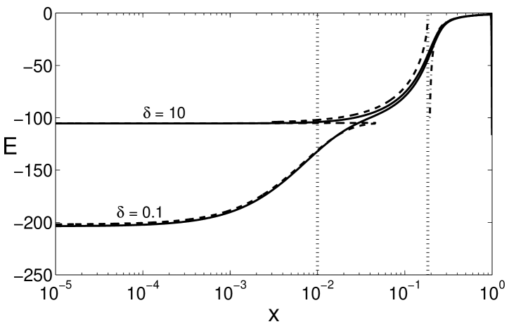
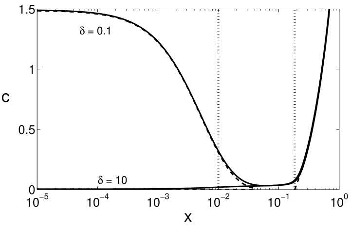
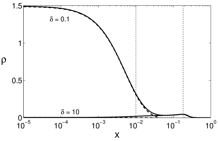
Fig. 4: Numerical solutions (solid lines) for the dimensionless electric field $E(x)$, average concentration $c(x)$, and charge density $\rho(x)$ above the diffusion-limited current ($j=1.5$) compared with leading order asymptotic approximations (dashed lines) for $k_{c}=1$, $j_{r}=2$, $\epsilon=0.01$, and $\delta=0.1,10$. The leading order bulk approximations are given by Eqs. (36). In the space-charge layer, the leading order electric field is given by Eq. (37), and leading order concentration is $0$. Finally, Eqs. (57) and (58) are the diffuse layer asymptotic approximations for the electric field and concentration, respectively. For reference, the vertical lines show where $x=\epsilon$ and $x=x_{o}$.

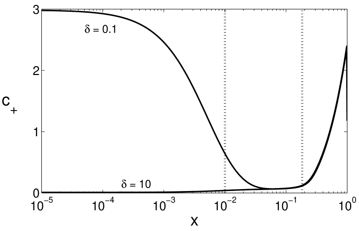
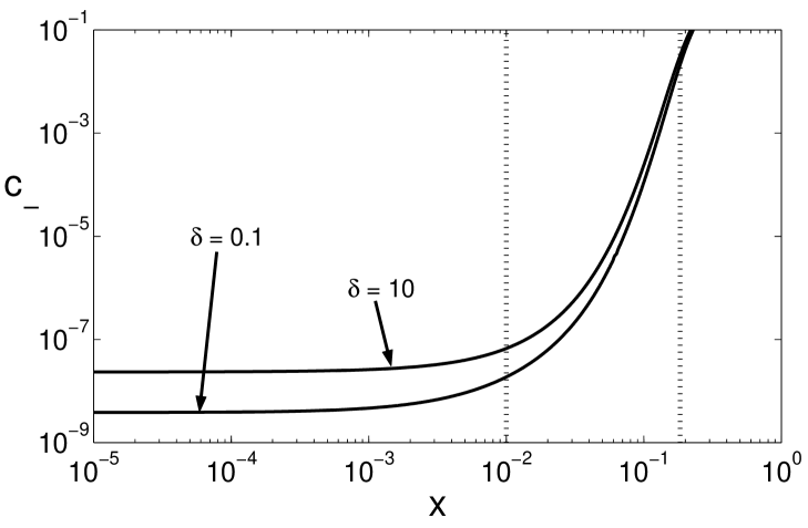
Fig. 5: Numerical solutions for the dimensionless cation and anion concentrations above the diffusion-limited current ($j=1.5$) for $k_{c}=1$, $j_{r}=2$, $\epsilon=0.01$, and $\delta=0.1,10$. For reference, the vertical lines show where $x=\epsilon$ and $x=x_{o}$.

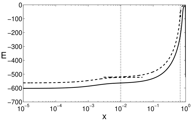
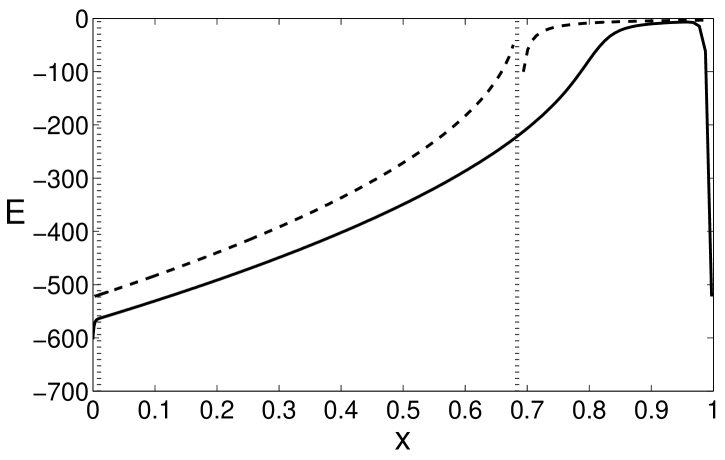
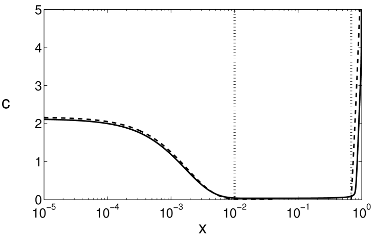
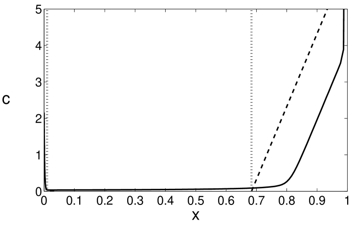
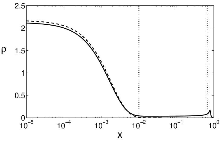
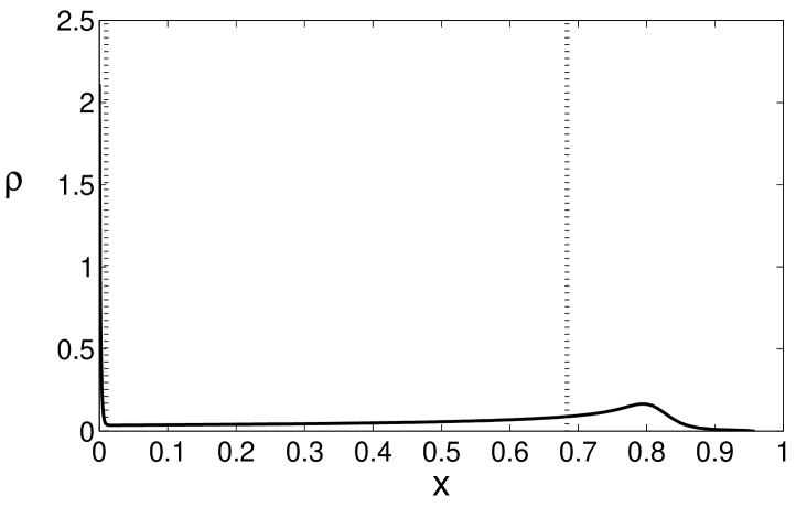
Fig. 6: Numerical solutions (solid lines) for the dimensionless electric field $E(x)$, average concentration $c(x)$, and charge density $\rho(x)$ far above the diffusion-limited current ($j=10.0$) compared with leading order asymptotic approximations (dashed lines) for $k_{c}=1$, $j_{r}=2$, $\epsilon=0.01$, and $\delta=0.1$. Each field is shown twice: (1) with $x$ on $\log$ scale to focus on the cathode region and (2) with $x$ on a linear scale to emphasize the interior of the cell. Note that $j\epsilon=0.1$, so the asymptotic approximations are not as good as at lower current densities. For reference, the vertical lines show where $x=\epsilon$ and $x=x_{o}$.

In between the two $O(1)$ layers, there is a small transition layer. Rescaling the master equation using the change of variables $z=(x-x_{o})/\epsilon^{2/3}$ and ${\acute{E}}(z)=\epsilon^{2/3}{\bar{E}}(x)$, we again obtain the Smyrl-Newman equation, Eq. (26), with right hand side equal to zero. As before, we find that the solution in the transition layer approaches $-1/z$ as $z\rightarrow\infty$. In the other direction as $z\rightarrow-\infty$, we will find that the appropriate boundary condition is ${\acute{E}}\rightarrow-2\sqrt{j|z|}$ to match the electric field in space-charge layer.

4.1 Structure of the Space-Charge Layer

Physically, we could argue that the concentration of ions in the space-charge layer is very small (i.e. zero at leading order) because the layer is essentially the result of stretching the ionic content of the overlap between the inner diffuse and Smyrl-Newman layers, which is small to begin with, over an $O(1)$ region. This physical intuition is confirmed by the numerical solutions shown in Figures 4, 5, and 6. Therefore, using Eq. (17), we obtain the leading order solution for the electric field

$${\tilde{E}}\sim\frac{-2\sqrt{j\left(x_{o}-x\right)}}{\epsilon}.$$ (37)

Note that the magnitude of the field is exactly what is required to make the integral term in $\b{c}_{o}$ an $O(1)$ contribution. From this formula, it is easy to compute the charge density in the space-charge layer

$${\tilde{\rho}}=\epsilon^{2}\frac{d{\tilde{E}}}{dx}\sim\epsilon\sqrt{\frac{j}{x_{o}-x}},$$ (38)

which is an order of magnitude larger than the $O(\epsilon^{2})$ charge density in the bulk. The $O(\epsilon)$ charge density also implies that the concentration must be at least $O(\epsilon)$ because the anion concentration, $c-\rho$, is positive.

With the electric field given by Eq. (37), we can determine the values of $x_{o}$ and $\b{c}_{o}$ by solving the system of equations given by the definition of $x_{o}$ and $\b{c}_{o}$. Using Eq. (18) to calculate $\b{c}_{o}$ and noticing that the leading order contribution to the integral comes from the space-charge layer, we obtain

$$\b{c}_{o}\sim 1-j(1+x_{o}^{2}).$$ (39)

Combining this result with $x_{o}=-\b{c}_{o}/2j$, we find that

$$x_{o}\sim 1-j^{-1/2}\ \ \ ,\ \ \ \b{c}_{o}\sim 2\left(j^{1/2}-j\right),$$ (40)

which can be substituted into Eqs. (36) and (37) to yield the leading order solutions in the bulk and space-charge layers. It should be noted that the expression for $x_{o}$ is consistent with the estimate for the width found by Bruinsma and Alexander [21] and Chazaviel [22] in the limits $j-1\ll 1$ and small space-charge layer ($x_{o}\ll 1$), although our analysis also applies to much larger voltages.

The results obtained via physical arguments in the previous few paragraphs motivate an asymptotic series expansion for $E$ whose leading order term is $O(1/\epsilon)$. Moreover, because we want to be able to balance the current density at second-order, we choose the second-order term to be $O(j)$. Thus, we have

$${\tilde{E}}=\frac{1}{\epsilon}E_{-1}+E_{0}j+\ldots.$$ (41)

Note that in this asymptotic series, the first term only dominates the second term as long as $j\ll 1/\epsilon$, so the following analysis only holds for current densities far below $O(1/\epsilon)$. Figure 6 illustrates the breakdown of the leading-order asymptotic solutions at very high current densities. While the qualitative features of the asymptotic approximation are correct (e.g. shape of $E(x)$ in the diffuse layer and slope of $c(x)$ in the bulk), the quality of the approximation is clearly less than at lower values of $j$.

The key advantage of a more systematic asymptotic analysis is that we are able to calculate the leading-order behavior of the space-charge layer concentration $\tilde{c}$, which is not possible with only knowledge of the leading order behavior for the electric field. Substituting Eq. (41) into the master equation (20), it is straightforward to obtain

$${\tilde{E}}\sim-\frac{2}{\epsilon}\sqrt{j\left(x_{o}-x\right)}-\frac{1}{2(x_{o}-x)}+\ldots.$$ (42)

Using this expression in Eq. (17), we find the dominant contribution to $\tilde{c}$ is exactly the same as ${\tilde{\rho}}$:

$$\tilde{c}\sim\epsilon\sqrt{\frac{j}{x_{o}-x}}.$$ (43)

Since $c_{-}=c-\rho$, this result leads to an important physical conclusion — The space-charge layer is essentially depleted of anions, $c_{-}=o(\epsilon)$, as is clearly seen in Figures 4 and 5. This contradicts our macroscopic intuition about electrolytes, but, in very thin films, complete anion deplection might occur. For example, in a microbattery developed for on-chip power sources using the Li/SiO₂/Si system, lithium ion conduction has recently been demonstrated in nano-scale films of silicon oxide, where there should not be any counter ions or excess electrons [6].

At leading order as $\epsilon\rightarrow 0$, the anion concentration, $c_{-}$, can be set to zero in the space-charge layer, leaving the following two governing equations:

$$\frac{dc_{+}}{dx}+c_{+}\frac{d\phi}{dx} = 4j$$ (44)

$$-\epsilon^{2}\frac{d^{2}\phi}{dx^{2}} = \frac{1}{2}c_{+}.$$ (45)

As with binary electrolyte case, these equations can be reduced to a single equation for the electric potential:

$$\frac{d^{3}\phi}{dx^{3}}+\frac{d^{2}\phi}{dx^{2}}\frac{d\phi}{dx}=-\frac{2j}{\epsilon^{2}}.$$ (46)

Integrating this equation once, we obtain a Riccati equation for $\frac{d\phi}{dx}$

$$\frac{d^{2}\phi}{dx^{2}}+\frac{1}{2}\left(\frac{d\phi}{dx}\right)^{2}=-\frac{2j}{\epsilon^{2}}(x-x_{o})+h,$$ (47)

where $h$ is an integration constant. Using the transformations

$$u\equiv e^{\phi/2}\ \ \ ,\ \ \ z\equiv-\frac{j^{1/3}}{\epsilon^{2/3}}\left(x-x_{o}\right)+\frac{\epsilon^{4/3}h}{2j^{2/3}},$$ (48)

we find that $u$ satifies Airy’s equation

$$\frac{d^{2}u}{dz^{2}}-zu=0.$$ (49)

Thus, the general solution for $\phi(x)$ is

$$\phi(x)=2\log\left[a_{1}Ai\left(\frac{j^{1/3}}{\epsilon^{2/3}}\left(x_{o}-x\right)+\beta h\right)+a_{2}Bi\left(\frac{j^{1/3}}{\epsilon^{2/3}}\left(x_{o}-x\right)+\beta h\right)\right],$$ (50)

where $a_{1}$ and $a_{2}$ are constants determined by boundary conditions and $\beta=\frac{\epsilon^{4/3}}{2j^{2/3}}$.

To simplify this expression, note that in the limit $\epsilon\rightarrow 0$, the potential drop between $x=x_{o}$ and $x=0$ is approximately

$$\phi(x_{o})-\phi(0)\sim 2\log\left[\frac{a_{1}Ai(0)+a_{2}Bi(0)}{a_{1}Ai\left(\frac{x_{o}j^{1/3}}{\epsilon^{2/3}}\right)+a_{2}Bi\left(\frac{x_{o}j^{1/3}}{\epsilon^{2/3}}\right)}\right].$$ (51)

Now, using the large argument behavior of the Airy functions, we see that as $\epsilon\rightarrow 0$, the argument of the logarithm approaches zero. Thus, we are lead to the conclusion that the electric potential at $x=x_{o}$ is less than at $x=0$. But, this is completely inconsistent with our physical intuition and the numerical results, which show that $\phi(x_{o})-\phi(0)>0$. Therefore, it must be the case that $a_{2}\approx 0$ so that

$$\phi(x)=2\log\left[a_{1}Ai\left(\frac{j^{1/3}}{\epsilon^{2/3}}\left(x_{o}-x\right)+\beta h\right)\right]$$ (52)

and

$$E(x)=\frac{2j^{1/3}}{\epsilon^{2/3}}\frac{Ai^{\prime}\left(\frac{j^{1/3}}{\epsilon^{2/3}}\left(x_{o}-x\right)+\beta h\right)}{Ai\left(\frac{j^{1/3}}{\epsilon^{2/3}}\left(x_{o}-x\right)+\beta h\right)}.$$ (53)

Finally, by using the asymptotic form of $Ai(z)$ and $Ai^{\prime}(z)$ as $z\rightarrow\infty$, we find that in the $\epsilon\rightarrow 0$ limit, the leading order approximation for the electric field when the region is depleted of anions is exactly Eq. (37).

That equivalence of the single-ion equations and the full governing equations at leading-order mathematically confirms the physically interpretation of the space-charge layer as a region of anion depletion. From an alternative perspective, it also reminds us that under extreme conditions, it may be necessary to rethink our assumptions about what physical effects are dominant.

4.2 Boundary Layers Above the Limiting Current

To complete our analysis of the high-current regime, $1+O(\epsilon^{2/3})\ll j\ll O(1/\epsilon)$, we must consider the boundary layers. At the anode, all fields are $O(1)$, so we recover the usual Gouy-Chapman solution with the minor modification that $c_{1}=2\sqrt{j}$ which is the value $\bar{c}$ takes as $x\rightarrow 1$. The cathode structure, however, is much more interesting because it is depleted of anions (see Figure 5). To our knowledge, this non-equilibrium inner boundary layer on the space-charge region, related to the reaction boundary condition at the cathode, has not been analyzed before.

As in the space-charge layer, the leading-order governing equations in this layer are those of a single ionic species with no counterions Eqns. (44) and (45). Rescaling those equations using $x=\epsilon y$, we obtain

$$\frac{d\check{c}_{+}}{dy}+\check{c}_{+}\frac{d{\check{\phi}}}{dy} = 4j\epsilon\approx 0$$ (54)

$$-\frac{d^{2}{\check{\phi}}}{dy^{2}} = \frac{1}{2}\check{c}_{+}.$$ (55)

From these equations, it is immediately clear that the cations have a Boltzmann equilibrium profile at leading order: $c_{+}\propto e^{-\phi(y)}$. As in the analysis for the space-charge layer, it is possible to find a general solution to Eqns. (54) and (55). By combining these equations and integrating, we find that the potential in the cathode boundary layer has the form

$${\check{\phi}}\sim\log\left[\sinh^{2}\left(py+q\right)\right]+r,$$ (56)

where $p$, $q$, and $r$ are integration constants. Therefore, the electric field and concentration are

$${\check{E}}(y) \sim -2p\coth\left(py+q\right)$$ (57)

$$\check{c}(y) = \frac{1}{2}\check{c}_{+}(y)\sim\frac{2p^{2}}{\sinh^{2}\left(py+q\right)}$$ (58)

Matching the electric fields in the diffuse and space-charge layers, we find that $p\sim\sqrt{jx_{o}}$. Note that because $p=O(\sqrt{j})$, the electric field in the diffuse charge layer is $O(\sqrt{j}/\epsilon)$ which is same order of magnitude as in the space-charge layer. To solve for $q$, we use the expression for $p$ in the cathode Stern and Butler-Volmer boundary conditions, which leads to the following nonlinear equation:

$$\frac{4k_{c}jx_{o}}{\sinh^{2}q}\exp\left(2\alpha_{c}\delta\sqrt{jx_{o}}\coth q\right)-j_{r}\exp\left(-2\alpha_{a}\delta\sqrt{jx_{o}}\coth q\right)=j.$$ (59)

In the limit of small $\delta$, we can use fixed-point iteration to obtain an approximate solution

$$q\sim\sinh^{-1}\left(2\sqrt{\frac{k_{c}jx_{o}\exp\left(2\alpha_{c}\delta\sqrt{jx_{o}}\coth q_{o}\right)}{j+j_{r}\exp\left(-2\alpha_{a}\delta\sqrt{jx_{o}}\coth q_{o}\right)}}\right)$$ (60)

where $q_{o}$ has the same form as $q$ with $(\coth q_{o})$ set equal to 1. For $\delta\gg 1$, the leading order equation is

$$\frac{4k_{c}jx_{o}}{\sinh^{2}q}\exp\left(2\alpha_{c}\delta\sqrt{jx_{o}}\coth q\right)\sim j,$$ (61)

which implies that $q\gg 1$ so that the left-hand side can be small enough to balance the current. Thus, by using $\coth q\approx 1$ and $\sinh q\approx\exp(q)/2$, we find that $q\sim\alpha_{c}\delta\sqrt{jx_{o}}+\frac{1}{2}\log(16k_{c}x_{o})$. The agreement of these asymptotic approximations with the exact solutions in the diffuse charge layer is illustrated in Figure 4.

5 Polarographic Curves

We are now in a position to compute the leading-order behavior of the polarographic curve at and above the classical limiting current. Recall that the formula for the cell voltage is given by

$$v=-\delta\epsilon E(0)+\int_{0}^{1}-E(x)dx-\delta\epsilon E(1).$$ (62)

The integral is the voltage drop through the interior of the cell and the first and last terms account for the potential drop across the Stern layers.

Table 1: Comparison of the asymptotic approximations Eqs. (64) and (65) with numerically calculated values for the cell voltage at various $\epsilon$ and $\delta$ values. These cell voltages were computed with $k_{c}=1$ and $j_{r}=2$.

$j$ = 1.0 $\epsilon$ $\delta$ $v_{exact}$ $v_{asym}$ 1e-4 0.01 13.125 12.101 1e-4 1.00 13.222 12.374 1e-4 10.0 14.290 13.571 1e-3 0.01 10.165 9.146 1e-3 1.00 10.277 9.475 1e-3 10.0 11.552 10.890 1e-2 0.01 7.339 6.303 1e-2 1.00 7.479 6.729 1e-2 10.0 9.228 8.465 1e-1 0.01 4.922 3.649 1e-1 1.00 5.005 4.219 1e-1 10.0 7.995 6.327

& $j$ = 1.5 $\epsilon$ $\delta$ $v_{exact}$ $v_{asym}$ 1e-4 0.01 1297.799 1289.621 1e-4 1.00 1297.048 1291.101 1e-4 10.0 1305.318 1300.129 1e-3 0.01 140.207 132.790 1e-3 1.00 139.450 134.270 1e-3 10.0 147.717 143.299 1e-2 0.01 22.434 15.725 1e-2 1.00 21.624 17.206 1e-2 10.0 29.886 26.234 1e-1 0.01 9.479 2.637 1e-1 1.00 7.790 4.118 1e-1 10.0 16.088 13.146 At the limiting current, $j=1$, we can estimate the voltage drop across the cell by using the bulk and diffuse layer electric field to approximate the field in the Smyrl-Newman transition layer to obtain

$$v \sim -\delta\epsilon E(0)+\int_{0}^{\epsilon^{2/3}}-E(x)dx+\int_{\epsilon^{2/3}}^{1}-E(x)dx-\delta\epsilon E(1)$$ (63)

$$\sim 2\frac{\delta}{b}+2\log\left(\frac{\epsilon^{-1/3}+b}{b}\right)-\frac{2}{3}\log\epsilon.$$ (64)

Notice that in the small $\delta$ limit, this expression reduces to $v\sim-\frac{4}{3}\ln\epsilon$ as $\epsilon\rightarrow 0$ which can be observed in the polarographic curves in Figure 6 in [9]. Table 5 compares this approximation with the exact cell voltage for a few $\epsilon$ and $\delta$ values. For small $\epsilon$ values ($\epsilon\leq 0.01$), the asymptotic approximations are fairly good (within 5% to 10%).

Above the limiting current, the space-charge layer makes the dominant contribution to the cell voltage. Using Eqns. (36) and (37) in the formula for the cell voltage, we find that

$$v \sim \frac{4\sqrt{j}}{3\epsilon}\left(1-j^{-1/2}\right)^{3/2}+2\delta\left(j-\sqrt{j}\right)^{1/2}\coth q-\frac{1}{2}\log j-2/3\log\epsilon.$$ (65)

The first two terms in this expression estimate the voltage drop across the space-charge and the cathode Stern layers, respectively. The last two terms are the subdominant contribution from the bulk where we have somewhat arbitrarily taken $x=x_{o}+\epsilon^{2/3}$ as the boundary between the bulk layer and the Smyrl-Newman transition layer. Notice that we ignore the contribution from the cathode diffuse and Smyrl-Newman layers. It is safe to neglect the diffuse layer because it is an $O(1)$ contribution. However, the Smyrl-Newman layer has a non-neglible potential drop that we have to accept as error since we do not have an analytic form for the solution in that region.

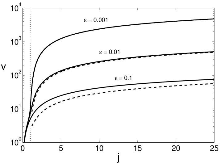
Fig. 7: Comparison of numerical polarographic curves (dashed lines) with leading-order asymptotic approximations (solid lines) given in Eq. (65) for several values of $\epsilon$ with $\delta=1.0$, $k_{c}=1$ and $j_{r}=2$. For $\epsilon=0.001$, the numerical and asymptotic polarographic curves are indistinguishable on this graph. For reference, the vertical, dashed line shows the classical diffusion-limited current $j=1$.

Figure 7 shows that the asymptotic polarographic curves are quite accurate for sufficiently small $\epsilon$ values. In Table 5, we compare the results predicted by the asymptotic formula with numerical results for a few specific values of $\epsilon$ and $\delta$. It is interesting that the approximation is also better for large $\delta$ values (we explain this observation in the next section). Also, while the $\log\epsilon$ term is subdominant, it makes a significant contribution to the cell voltage for $\epsilon$ values as small as $0.01$.

As with the width of the space-charge layer, $x_{o}$, our expression for the cell voltage, Eq. (65), is consistent with the results of Bruinsma and Alexander [21] and Chazaviel [22], near the limiting curent, $j\rightarrow 1^{+}$, while remaining valid at much larger currents, $j=O(1/\epsilon)$

6 Effects of the Stern-Layer Capacitance

The inclusion of the Stern layer in the boundary conditions allows us to explore the effects of the intrinsic surface capacitance on the structure of the cell. From Figures 3 through 5, we can see that smaller Stern-layer capacitances (i.e. larger $\delta$ values) decrease the concentration and electric field strength in the cathode diffuse layer. This behavior arises primarily from the influence of the electric field on the chemical kinetics at the electrode surfaces. When the capacitance of the Stern layer is low, small electric fields at the cathode surface translate into large potential drops across the Stern layer, Eq. (10), which help drive the deposition reaction, Eq. (12). As a result, neither the electric field nor the cation concentration need to be very large at the cathode to support high current densities. These results confirm our physical intuition that it is only important to pay attention to the diffuse layer when the Stern layer potential drop is negligible (i.e $\delta\ll 1$).

At high currents, another important effect of the Stern layer capacitance is that the total cell voltage becomes dominated by the potential drop across the Stern layer at large $\delta$ values (i.e. small capacitances). This behavior is clearly illustrated in Figure 8. Notice for currents below the classical diffusion-limited current, the total cell voltage does not show a strong dependence on $\delta$. However, for $j>1$, the total cell voltage increases with $\delta$ – the increase being driven by the strong $\delta$ dependence of the Stern voltage.

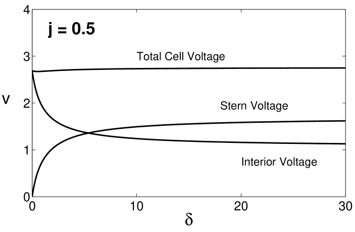
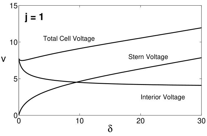
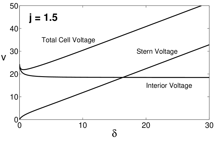
Fig. 8: These graphs break the total cell voltage into contributions from the cell interior and the Stern layer as a function of $\delta$ for $\epsilon=0.01$, $k_{c}=2$, and $j_{r}=2$. Note that at and above the classical limiting current, the Stern layer voltage dominates the total cell voltage for large values of $\delta$.

7 Conclusion

In summary, we have studied classical problem of direct current in an electrochemical cell, focusing on the exotic regime of high current densities. A notable new feature of our study is the use of nonlinear Butler-Volmer and Stern boundary conditions to model a thin film passing a Faradaic current, as in a micro-battery. We have derived leading-order approximations for the fields at and above the classical, diffusion-limited current, paying special attention to the structure of the cathodic boundary layer, which must be present to satisfy the reaction boundary conditions. In our analysis of superlimiting current, we have shown that the key feature of the bulk space-charge layer is the depletion of anions. Our exact solution of the leading-order problem in the space-charge region, Eq. (50), could thus also have relevance for Faradaic conduction through very thin insulating films.

Using the asymptotic approximations to the fields, we are able to derive a current-voltage relation, Eq. (65), which compares well with numerical results, far beyond the limiting current. Combined with the analogous formulae in the companion paper [9], which hold below the limiting current, we have essentially analyzed the full range of the current-voltage relation. These results could be useful in interpreting experimental data, e.g. on the internal resistance of thin-film microbatteries.

A general conclusion of this study is that boundary conditions strongly affect the solution. For example, the Stern-layer capacitance, often ignored in theoretical analysis, plays an important role in determining the qualitative structure of the cell near the cathode, as well as the total cell voltage. The nonlinear boundary conditions for Butler-Volmer reaction kinetics also profoundly affect charge distribution and current-voltage relation, compared to the ubiquitous case of Dirichlet boundary conditions. The latter rely on the asumption of surface equilibrium, which is of questionable validity at very large currents.

We leave the reader with a word of caution. The results presented here are valid mathematical solutions of standard model equations, but their physical relevance should be met with some skepticism under extreme conditions, such as superlimiting current. For example, the PNP equations are meant to describe infinitely dilute solutions in relatively small electric fields [7, 27, 28]. Even for quasi-equilibrium double layers, their validity is not so clear when the zeta potential greatly exceeds the thermal voltage, because co-ion concentrations may exceed the physical limit required by discreteness (accounting also for solvation shells) and counter-ion concentations may become small enough to violate the continuum assumption. Large electric fields can cause the permittivity to vary, by some estimates up to a factor ten, as solvent dipoles become aligned. Including such effects, however, introduces further ad hoc parameters into the model, which may be difficult to infer from experimental data.

8 Acknowledgments

This work was supported in part by the MRSEC Program of the National Science Foundation under award number DMR 02-13282 and in part by the Department of Energy through the Computational Science Graduate Fellowship (CSGF) Program provided under grant number DE-FG02-97ER25308. The authors thank M. Brenner, J. Choi, and B. Kim for helpful discussions.

References

- [1] . N. J. Dudney, J. B. Bates, D. Lubben, and F. X. Hart, Thin-Film Rechargeable Lithium Batteries with Amorphous LixMn2O4 cathodes, in Thin Film Solid Ionic Devices and Materials, J. Bates, The Electrochemical Society, Pennington, NJ, 1995, pp. 201-214.
- [2] . B. Wang, J. B. Bates, F. X. Hart, B. C. Sales, R. A. Zuhr, and J. D. Robertson, Characterization of Thin-Film Rechargeable Lithium Batteries with Lithium Cobalt Oxide Cathodes, J. Electrochem. Soc., 143 (1996), pp. 3204-3213.
- [3] B. J. Neudecker, N. J. Dudney, J. B. Bates, “Lithium-Free” Thin-Film Battery with In Situ Plated Li Anode, J. Electrochem. Soc., 147 (2000), pp. 517–523.
- [4] N. Takami, T. Ohsaki, H. Hasabe, and M. Yamamoto, Laminated Thin Li-Ion Batteries Using a Liquid Electrolyte, J. Electrochem. Soc., 149 (2002), pp. A9–A12.
- [5] Z. Shi, L. Lü, and G. Ceder, Solid State Thin Film Lithium Microbatteries, Singapore-MIT Alliance Technical Report: Advanced Materials for Micro- and Nano-Systems Collection, Jan. 2003. http://hdl.handle.net/1721.1/3672.
- [6] N. Ariel, E. Fitzgerald, and D. Sadoway, in preparation.
- [7] J. Newman, Electrochemical Systems, Prentice-Hall, Inc., Englewood Cliffs, NJ, 1991.
- [8] I. Rubinstein, Electro-Diffusion of Ions, SIAM Studies in Applied Mathematics, SIAM, Philadelphia, PA, 1990.
- [9] M. Z. Bazant, K. T. Chu, and B. J. Bayly, Current-voltage relations for electrochemical thin films, preprint.
- [10] W. Nernst, , Z. Phys. Chem., 47 (1904), pp. 52–55.
- [11] V. G. Levich, Physico-chemical Hydrodynamics, Prentice-Hall, London, 1962.
- [12] A. A. Chernenko, The theory of the passage of direct current through a solution of a binary electrolyte, Dokl. Akad. Nauk. SSSR, 153 (1962), p. 1129–1131. (English translation, pp. 1110–1113.)
- [13] J. Newman, The Polarized Diffuse Double Layer, Trans. Faraday Soc., 61 (1965), pp. 2229–2237.
- [14] A. D. MacGillivray, Nernst-Planck equations and the electroneutrality and Donnan equilibrium assumptions, J. Chem. Phys. 48 (1968), pp. 2903–2907.
- [15] W. H. Smyrl and J. Newman, Double Layer Structure at the Limiting Current, Trans. Faraday Soc., 63 (1967), pp. 207–216.
- [16] I. Rubinstein and L. Shtilman, Voltage against Current Curves of Cation Exchange Membranes, J. Chem. Soc. Faraday. Trans. II, 75 (1979), pp. 231–246.
- [17] S. S. Dukhin, Electrokinetic phenomena of the second kind and their applications, Adv. Colloid Interface Sci., 35 (1991) pp. 173-196.
- [18] Y. Ben and H.-C. Chang, Nonlinear Smoluchowski slip velocity and micro-vortex generation, J. Fluid. Mech., 461 (2002), pp. 229–238.
- [19] I. Rubinstein and B. Zaltzman, Electro-osmotically induced convection at a permselective membrane, Phys. Rev. E, 62 (2000), pp. 2238–2251.
- [20] I. Rubinstein and B. Zaltzman, Electro-osmotic slip of the second kind and instability in concentration polarization at electrodialysis membranes, Math. Models Meth. Appl. Sci., 2(2000), pp. 263–299.
- [21] R. Bruinsma and S. Alexander, Theory of electrohydrodynamic instabilities in electrolytic cells, J. Chem. Phys., 92 (1990), pp. 3074–3085.
- [22] J.-N. Chazalviel, Electrochemical aspects of the generation of ramified metallic electrodeposits, Phys. Rev. A, 42 (1990), pp. 7355–7367.
- [23] A. Bonnefont, F. Argoul, and M. Z. Bazant, Analysis of diffuse-layer effects on time-dependent interfacial kinetics, J. Electroanal. Chem., 500 (2001), pp. 52–61.
- [24] B. M. Grafov and A. A. Chernenko, Dokl. Akad. Nauk. SSSR, 146 (1962), pp. 135–138. (In Russian.)
- [25] J. P. Boyd, Chebyshev and Fourier Spectral Methods, Dover Publications, Inc., Mineola, NY, 2001.
- [26] L. N. Trefethen, Spectral Methods in MATLAB, SIAM, Philadelphia, PA, 2000.
- [27] P. Delahay, Double Layer and Electrode Kinetics, Interscience Publishers, New York, NY, 1965.
- [28] A. J. Bard and L. R. Faulkner, Electrochemical Methods, John Wiley & Sons, Inc., New York, NY, 2001.