Current-voltage relations for electrochemical thin films

Abstract

The dc response of an electrochemical thin film, such as the separator in a micro-battery, is analyzed by solving the Poisson-Nernst-Planck equations, subject to boundary conditions appropriate for an electrolytic/galvanic cell. The model system consists of a binary electrolyte between parallel-plate electrodes, each possessing a compact Stern layer, which mediates Faradaic reactions with nonlinear Butler-Volmer kinetics. Analytical results are obtained by matched asymptotic expansions in the limit of thin double layers and compared with full numerical solutions. The analysis shows that (i) decreasing the system size relative to the Debye screening length decreases the voltage of the cell and allows currents higher than the classical diffusion-limited current; (ii) finite reaction rates lead to the important possibility of a reaction-limited current; (iii) the Stern-layer capacitance is critical for allowing the cell to achieve currents above the reaction-limited current; and (iv) all polarographic (current-voltage) curves tend to the same limit as reaction kinetics become fast. Dimensional analysis, however, shows that “fast” reactions tend to become “slow” with decreasing system size, so the nonlinear effects of surface polarization may dominate the dc response of thin films.

Introduction

Micro-electrochemical systems pose interesting problems for applied mathematics because traditional “macroscopic” approximations of electroneutrality and thermal equilibrium [1], which make the classical transport equations more tractable [2], break down at small scales, approaching the Debye screening length. Of course, the relative importance of surface phenomena also increases with miniaturization. Micro-electrochemical systems of current interest include ion channels in biological membranes [3, 4, 5] and thin-film batteries [6, 7, 8, 9, 10], which could revolutionize the design of modern electronics with distributed on-chip power sources. In the latter context, the internal resistance of the battery is related to the nonlinear current-voltage characteristics of the separator, consisting of a thin-film electrolyte (solid, liquid, or gel) sandwiched between flat electrodes and interfacial layers where Faradaic electron-transfer reactions occur [11]. Under such conditions, the internal resistance is unlikely to be simply constant, as is usually assumed.

Motivated by the application to thin-film batteries, here we revisit the classical problem of steady conduction between parallel, flat electrodes, studied by Nernst [12] and Brunner [13, 14] a century ago. As in subsequent studies of liquid [15, 16] and solid [17, 18] electrolytes, we do not make Nernst’s assumption of bulk electroneutrality and work instead with the Poisson-Nernst-Planck (PNP) equations, allowing for diffuse charge in solution [1, 2]. What distinguishes our analysis from previous work on current-voltage relations (or “polarographic curves”) is the use of more realistic nonlinear boundary conditions describing (i) Butler-Volmer reaction kinetics and (ii) the surface capacitance of the compact Stern layer, as in the recent paper of Bonnefont et. al [19]. Such boundary conditions, although complicating mathematical analysis, generally cannot be ignored in micro-electrochemical cells, where interfaces play a crucial role. Diffuse-charge dynamics, which can be important for high-power applications, also complicates analysis [20], but in most cases it is reasonable to assume that electrochemical thin films are in steady state, due to the short distances for electro-diffusion.

We stress, however, that steady state does not imply thermal equilibrium when the system sustains a current, driven by an applied voltage. In this paper, we focus on applied voltages small enough to justify the standard boundary-layer analysis of the PNP equations, which yields charge densities in thermal equilibrium at leading order in the limit of thin double layers [21]. In a companion paper [22], we extend the analysis to larger voltages, at [23] and above [24] the Nernst’s diffusion-limited current, and show how more realistic boundary conditions affect diffuse charge, far from thermal equilibrium. In both cases, we obtain novel formulae for polarographic curves by asymptotic analysis in the limit of thin double layers, which we compare with numerical solutions, and we focus on a variety of dimensionless physical parameters: the reaction-rate constants (scaled to the typical diffusive flux) and the ratios of the Stern length to the Debye length to the electrode separation.

1 Mathematical Model

Let us consider uniform conduction through a dilute, binary electrolyte between parallel plate electrodes separated by a distance, $L$. Our goal is to determine the steady-state response of the electrochemical cell to either an applied voltage, $V$, or an applied current, $I$. Specifically, we seek the electric potential $\Phi(X)$ and the concentrations $C_{+}(X)$ and $C_{-}(X)$ of cations and anions in the region $0\leq X\leq L$. The Faradaic current is driven by redox reactions occurring at the electrodes, and we neglect any other chemical reactions, such as dissociation/recombination in the bulk solution or hydrogen production. Since we do not assume electroneutrality, the region of integration extends to the point where the continuum approximation breaks down near each electrode, roughly a few molecules away. In other words, our integration region includes the “diffuse part” but not the “compact part” of the double layer [1, 11, 25, 26].

1.1 Transport Equations.

In the context of dilute solution theory [1, 2], the governing equations for this situation are the steady PNP equations:

$$\frac{d}{dX}\left(D_{+}\frac{dC_{+}}{dX}+\mu_{+}z_{+}FC_{+}\frac{d\Phi}{dX}\right)=0$$ (1)

$$\frac{d}{dX}\left(D_{-}\frac{dC_{-}}{dX}+\mu_{-}z_{-}FC_{-}\frac{d\Phi}{dX}\right)=0$$ (2)

$$-\frac{d}{dX}\left(\epsilon_{s}\frac{d\Phi}{dX}\right)=(z_{+}C_{+}-z_{-}C_{-})F.$$ (3)

where $F$ is Faraday’s constant (a mole of charge), $z_{\pm}$, $\mu_{\pm}$, and $D_{\pm}$ are the charge numbers, mobilities, and diffusivities of each ionic species, respectively, and $\epsilon_{s}$ is the permittivity of the solvent, all taken to be constant in the limit of infinite dilution. The first two equations set divergences of the ionic fluxes to zero in order to maintain the steady state, and the third is Poisson’s equation relating the electric potential to the charge density. In each flux expression, the first term represents diffusion and the second electromigration. The Einstein relation, $\mu_{\pm}=D_{\pm}/RT$, relates mobilities and diffusion coefficients via the absolute temperature, $T$, and the universal gas constant, $R$.

Due to the potentially large electric fields in thin films, as in interfacial double layers, these classical approximations could break down [1, 25, 26]. For example, the polarization of solvent molecules in large electric fields can lower the solvent dielectric permittivity by an order of magnitude, while also affecting the diffusivity and mobility. The solution can also become locally so concentrated or depleted of certain ions as to make finite sizes and/or interactions (and thus ionic activities) important. In spite of these concerns, however, it is reasonable to analyze the PNP equations before considering more complicated transport models, especially because our focus is on the effect of boundary conditions.

1.2 Electrode Boundary Conditions

Although PNP equations constitute a well-understood and widely accepted approximation, appropriate boundary conditions for them are not so clear, and drastic approximations, such as constant concentration, potential or surface charge (or zeta potential), are usually made, largely out of mathematical convenience. On the other hand, in the context of electric circuit models for electrochemical cells [20, 27, 28], much effort has been made to describe the nonlinear response of the electrode-electrolyte interface, while describing the bulk solution as a simple circuit element, such as resistor. Here, we formulate general boundary conditions based on classical models of the double layer [11, 25, 26], with a unified description of ion transport by the PNP equations.

Our first pair of boundary conditions sets the normal anion flux to zero at each electrode,

$$D_{-}\frac{dC_{-}}{dX}(0)+\mu_{-}z_{-}FC_{-}(0)\frac{d\Phi}{dX}(0) = 0$$ (4)

$$D_{-}\frac{dC_{-}}{dX}(L)+\mu_{-}z_{-}FC_{-}(L)\frac{d\Phi}{dX}(L) = 0,$$ (5)

on the assumption that anions do not specifically adsorb onto the surfaces, which holds for many anions at typical metal surfaces (e.g. SO${}_{4}^{-2}$, OH^-, F^-). The second pair relates the normal cation flux to the net deposition (or dissolution) flux, or reaction-rate density, $R(C_{+},\Delta\Phi_{S})$, which in the dilute limit is assumed to depend only on cation concentration and potential drop, $\Delta\Phi_{S}$, across the compact part of the double layer, originally proposed by Stern [30]. Following the convention in electrochemistry, we take $\Delta\Phi_{S}$ to be the potential of the electrode surface measured relative to the solution. The reference potential is chosen so that the cathode, located at $X=0$, is at zero potential and the anode, located at $X=1$, is at the applied cell voltage $V$. Therefore, we have the following two boundary conditions,

$$D_{+}\frac{dC_{+}}{dX}(0)+\mu_{+}z_{+}FC_{+}(0)\frac{d\Phi}{dX}(0) = R\left(C_{+}(0),\Phi(0)\right)$$ (6)

$$-D_{+}\frac{dC_{+}}{dX}(L)-\mu_{+}z_{+}FC_{+}(L)\frac{d\Phi}{dX}(L) = R\left(C_{+}(L),\Phi(L)-V)\right).$$ (7)

For electrodes, it is typical to assume a balance of forward (deposition) and backward (dissolution) reaction rates biased by the Stern voltage with an Arrhenius temperature dependence,

$$R(C_{+},\Delta\Phi_{S})=K_{c}C_{+}\exp\left(\frac{-\alpha_{c}zF\Delta\Phi_{S}}{RT}\right)-K_{a}C_{M}\exp\left(\frac{\alpha_{a}zF\Delta\Phi_{S}}{RT}\right),$$ (8)

where $C_{M}$ is the (constant) density of electrode metal and $K_{c}$ and $K_{a}$ are rate constants for the cathodic and anodic reactions [1]. (Expressing the reaction rate in terms of the surface overpotential, $\eta_{S}=\Delta\Phi_{S}-\Delta\Phi_{S}^{eq}$, where $\Delta\Phi_{S}^{eq}$ is the Stern-layer voltage in the absence of current, $R=0$, yields the more common form of the Butler-Volmer equation [1, 26].) The Stern layer voltage contributes $-zF\Delta\Phi_{S}$ to the activation energy barriers multiplied by transfer coefficients $\alpha_{c}$ and $\alpha_{a}$ for the cathodic and anodic reactions, respectively, where $\alpha_{c}\approx\alpha_{a}\approx\frac{1}{2}$, for single electron transfer reactions [1, 26, 29].

Following Frumkin [31], we apply Eq. (8) just outside the Stern layer, in contrast to “macroscopic” models which postulate the Butler-Volmer equation as a purely empirical description of reactions between the electrode surface and the electrically neutral bulk solution. Physically, the Frumkin approach makes more sense since the activation energy barrier described by the Butler-Volmer equation actually exists at the atomic scale in the Stern layer, not across the entire “interface” including diffuse charge in solution. We are not aware of any prior analysis with the full, nonlinear Butler-Volmer equation as a boundary condition on the PNP equations other than that of Bonnefont et al. [19]. Earlier analyses by Jaffé et. al.[15, 16] and Itskovich et. al.[17] also include electrode reactions, but only for small perturbations around equilibrium.

The final pair of boundary conditions determines the electric potential by specifying the voltage drop across the Stern layer in terms of the local electric field and concentrations,

$$0-\Phi(0) = \Delta\Phi_{S}\left(\frac{d\Phi}{dX}(0),C_{+}(0),C_{-}(0)\right)$$ (9)

$$V-\Phi(L) = \Delta\Phi_{S}\left(-\frac{d\Phi}{dX}(L),C_{+}(L),C_{-}(L)\right).$$ (10)

In macroscopic electrochemistry, these boundary conditions are usually replaced by the assuption of electroneutrality (which eliminates the need to solve Poisson’s equation) or by simple Dirichlet boundary conditions on the potential [1]. In colloidal science, they are likewise replaced by simple boundary conditions of constant surface charge (or zeta potential) [32, 33]. Here, we incorporate more realistic properties of the interface as follows: Neglecting the specific adsorption of anions, the Stern layer acts as a nonlinear capacitor in series with the diffuse layer. Grahame’s celebrated electrocapillary measurements [34, 35] suggest that $(i)$ the Stern layer capacitance, $C_{S}$, is roughly independent of concentration, depending mainly on the (variable) total charge, $\sigma$,

$$\frac{d(\Delta\Phi_{S})}{d\sigma}=\frac{1}{C_{S}(\sigma)},$$ (11)

and $(ii)$ dilute solution theory accurately describes the capacitance, $C_{D}(\sigma,C_{+})$, of the diffuse layer, at least when the charge and current are small enough to be well-described by Poisson-Boltzmann theory (as derived below). Using Gauss’ law, the surface charge density can be expressed in terms of the normal electric field, $\sigma=-\epsilon_{S}d\Phi/dX$, where $\epsilon_{S}$ is an effective permittivity of the compact layer. Therefore, integrating Eq. (11), Grahame’s model corresponds to the assumption,

$$\Delta\Phi_{S}=\int_{0}^{-\epsilon_{S}d\Phi/dx}\frac{d\sigma}{C_{S}(\sigma)},$$ (12)

which determines how the voltage across the compact layer (relative to the point of zero charge for which $\Delta\Phi_{S}=0$) varies as the two capacitors become charged. The function, $C_{S}(\sigma)$, should be fit to experimental or theoretical electrocapillary curves at large concentrations (since $1/C_{total}=1/C_{D}+1/C_{S}\approx 1/C_{S}$ in that case).

The simplest model that captures this interplay between the compact and diffuse layers is the Stern model [11, 26], which assumes the capacitance of the compact layer, $C_{S}$, to be constant [30]. While more complicated models for the compact layer have been proposed [36, 37, 25], the Stern model suffices for our purposes, because it allows us to describe surface capacitance easily in the context of our model of Faradaic reactions. Following Itskovich et al. [17] and Bonnefont et al. [19], let us introduce an effective width, $\lambda_{S}$, for the compact layer, $\lambda_{S}=\epsilon_{S}/C_{S}$, so that Eq. (12) reduces to a linear extrapolation of the potential across the compact layer, $-\Delta\Phi_{S}=\lambda_{S}d\Phi/dx$. Substituting this expression into Eqs. (9) and (10) yields two Robin boundary conditions,

$$\Phi(0)-\lambda_{S}\frac{d\Phi}{dX}(0) = 0$$ (13)

$$\Phi(L)+\lambda_{S}\frac{d\Phi}{dX}(L) = V,$$ (14)

completing a set of six boundary conditions for our three second-order differential equations. Physically, the Stern layer, as an effective solvation shell for the electrode, is only a few molecules wide, so it is best to think of $\lambda_{S}$ as simply a measure of the capacitance of the Stern layer. More generally, the same boundary condition could also describe a thin dielectric layer on the electrode [38, 39, 40], e.g. arising from surface contamination or a passivating monolayer.

Note that since the anion flux is zero, the current passing through the cell is proportional to the cation flux (everywhere in the cell, since it is constant),

$$I=z_{+}FA\left(D_{+}\frac{dC_{+}}{dX}+\mu_{+}z_{+}FC_{+}\frac{d\Phi}{dX}\right),$$ (15)

where $A$ is the electrode area and a current flow towards the cathode ($x=0$) is taken to be positive. Under potentiostatic conditions, the cell voltage $V$ is given, and the steady-state polarization curve $I(V)$ is determined by solving the equations. Conversely, under galvanostatic conditions, $I$ is fixed, and we solve for $V(I)$.

1.3 An Integral Constraint

As formulated above, the boundary value problem is not well-posed. Since the anion flux is constant throughout the cell according to Eq. (2), the two anion flux boundary conditions are degenerate, leaving one constant of integration undetermined. This is not surprising as we have omitted one crucial physical parameter, the total number of anions. More precisely, because anions do not react, we must specify their total number, which remains constant as the steady state is reached. This corresponds to the constraint,

$$\frac{1}{L}\int_{0}^{L}C_{-}(X)dX=C_{ref},$$ (16)

where $C_{ref}$ is the initial concentration of anions.

Note that the total number of cations (and hence the total charge) is not known a priori because the removal of cations at the cathode and the injection of cations at the anode may significantly alter their total number. This may seem counter-intuitive since we are accustomed to assuming that we know the total cation concentration at all times based on the original molarity of the solution, but this “macroscopic” thinking does not apply when the physics at the microscopic level are explicitly being studied (e.g. diffuse charge layers or micro-electrochemical systems). Mathematically, the reaction boundary conditions at the electrodes Eqs. (6) and (7) are sufficient to determine the total cation concentration (and total charge), as long as the total anion concentration is specified.

1.4 Dimensionless Formulation

To facilitate our analysis, we formulate the problem in dimensionless form. For simplicity we also assume that the electrolyte is symmetric, $z_{+}=-z_{-}\equiv z$, which does not qualitatively affect any of our conclusions as long as $z_{+}/|z_{-}|$ is not too different from $1$ (which holds for most simple, aqueous electrolytes). Scaling the basic variables as follows,

$$x\equiv X/L,\ \ \ c_{\pm}(x)\equiv C_{\pm}(xL)/C_{ref},\ \ \ \phi(x)\equiv\frac{zF\Phi(xL)}{RT},$$ (17)

Eqs. (1)–(3) become

$$\frac{d^{2}c_{+}}{dx^{2}}+\frac{d}{dx}\left(c_{+}\frac{d\phi}{dx}\right)=0$$ (18)

$$\frac{d^{2}c_{-}}{dx^{2}}-\frac{d}{dx}\left(c_{-}\frac{d\phi}{dx}\right)=0$$ (19)

$$-\epsilon^{2}\frac{d^{2}\phi}{dx^{2}}=\frac{1}{2}(c_{+}-c_{-})$$ (20)

where $\epsilon\equiv\lambda_{D}/L$ is the ratio of the Debye screening length $\lambda_{D}\equiv\sqrt{\frac{\epsilon_{s}RT}{2z^{2}F^{2}C_{ref}}}$ to the distance between electrodes. The Debye length is typically on the order of nanometers, so $\epsilon$ is always extremely small for macroscopic electrochemical cells. This situation changes, however, as $L$ or $C_{ref}$ is decreased, and in the case of nano-electrochemical systems $\epsilon$ could be as large as $10$.

The two flux equations are easily integrated, using Eq. (4) to evaluate one constant and leaving the other constant expressed in terms of the current via Eq. (15),

$$\frac{dc_{+}}{dx}+c_{+}\frac{d\phi}{dx} = 4j$$ (21)

$$\frac{dc_{-}}{dx}-c_{-}\frac{d\phi}{dx} = 0,$$ (22)

where we have defined a dimensionless current density, $j\equiv I/I_{d}$, scaled to the Nernst’s diffusion-limited current density (see Section 2.1), $I_{d}\equiv 4zFD_{+}C_{ref}A/L$. Since diffuse charge is of primary interest here, it is convenient to introduce

$$c=\frac{1}{2}(c_{+}+c_{-})\ \ \ \textrm{and}\ \ \ \rho=\frac{1}{2}(c_{+}-c_{-}),$$ (23)

the average concentration of ions and (half) the charge density, respectively, which leaves us with a coupled set of one second-order and two first-order differential equations,

$$\frac{dc}{dx}+\rho\frac{d\phi}{dx}=2j$$ (24)

$$\frac{d\rho}{dx}+c\frac{d\phi}{dx}=2j$$ (25)

$$-\epsilon^{2}\frac{d^{2}\phi}{dx^{2}}=\rho.$$ (26)

Nondimensionalizing the boundary conditions (remembering that there is an extra condition needed to determine the current-voltage relation, $j(v)$ or $v(j)$), we obtain:

$$\phi(0)-\delta\epsilon\frac{d\phi}{dx}(0) = 0,$$ (27)

$$\phi(1)+\delta\epsilon\frac{d\phi}{dx}(1) = v,$$ (28)

$$k_{c}[c(0)+\rho(0)]e^{\alpha_{c}\phi(0)}-j_{r}e^{-\alpha_{a}\phi(0)} = j,$$ (29)

$$-k_{c}[c(1)+\rho(1)]e^{\alpha_{c}(\phi(1)-v)}+j_{r}e^{-\alpha_{a}(\phi(1)-v)} = j,$$ (30)

$$\int_{0}^{1}[c(x)-\rho(x)]dx = 1,$$ (31)

where

$$k_{c}\equiv\frac{K_{c}L}{4D_{+}},\ \ \ j_{r}\equiv\frac{K_{a}LC_{M}}{4D_{+}C_{ref}},\ \ \ v\equiv\frac{zFV}{RT},\ \ \mbox{ and}\ \delta\equiv\frac{\lambda_{S}}{\lambda_{D}}.$$ (32)

Keep in mind that the dimensionless rate constants decrease with system size, so that “fast reactions” ($k_{c},j_{r}\gg 1$) may become “slow reactions” ($k_{c},j_{r}=O(1)$) as $L$ is reduced to the micron or submicron scale.

It is important to note that we have scaled the effective Stern layer width, $\lambda_{S}$, with the Debye screening length, $\lambda_{D}$, rather than the electrode separation $L$, thus introducing the factor $\epsilon=\lambda_{D}/L$ in Eqs. (27) and (28). This choice is important for our asymptotic analysis of the limit $\epsilon\rightarrow 0$ at fixed $\delta$, which is intended to describe situations in which $L$ is much larger than both $\lambda_{S}$ and $\lambda_{D}$. Without it, our analysis would assume that as $\epsilon\rightarrow 0$ the Stern layer becomes infinitely wide compared to the diffuse layer, even though it is mainly the macroscopic electrode separation which varies. The limit of very small Stern layer capacitance, which amounts to the Helmoltz model of the double layer [41], is best studied by letting $\delta\rightarrow\infty$ after $\epsilon\rightarrow 0$. In contrast, because $\epsilon$ and $\delta$ would both be small, the limit of very large Stern layer capacitance can be studied by simply letting $\delta=0$, yielding the Dirichlet boundary conditions,

$$\phi(0)=0\ \ \ ,\ \ \ \phi(1)=1,$$ (33)

of the Gouy-Chapman model of the double layer [42, 43]. In our work, we shall consider both limits, starting with the assumption that $\delta=O(1)$, which corresponds to the Gouy-Chapman-Stern model of the double layer [11, 26].

For one-dimensional problems, galvanostatic conditions are more mathematically convenient than potentiostatic conditions. In the former case, $j$ is given, and $v(j)$ is easily obtained from the Stern boundary condition at the anode Eq. (28). In the latter case, however, $v$ is specified and $j(v)$ must be determined self-consistently to satisfy Eq. (28). Therefore, we shall assume that the current $j$ is specified and solve Eqs. (24)–(26) subject to the boundary conditions Eqs. (29) and (30) and the integral constraint Eq. (31).

2 Boundary-layer Analysis

In this section, we briefly review the classical asymptotic analysis of the PNP equations, pioneered independently by Chernenko [44], Newman [21], and MacGillivray [45], which involves boundary layers of width, $\epsilon$ (corresponding to diffuse-charge layers of dimensional width, $\lambda_{D}$). As discussed below, the classical asymptotics breaks down at large currents approaching diffusion limitation. Unlike most previous authors, who assume either a fixed potential [42, 43] or fixed interfacial charge [21] at an isolated electrode or fixed concentrations at cell boundaries with ion-permeable membranes [4, 5, 24], we solve for the response of a complete, two-electrode galvanic cell with boundary conditions for Faradaic reactions and Stern-layer capacitance.

Throughout this section, the reader may refer to Figure  1, which compares the uniform asymptotic solutions derived below to numerical solutions at several values of $\epsilon$. These figures illustrate the structure of the field variables in the cell as well as give an indication of the quality of the asymptotic solutions. The numerical solutions are obtained by a straightforward iterative spectral method, described in a companion paper [22].

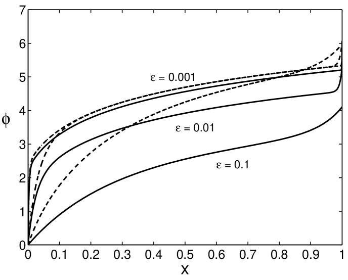
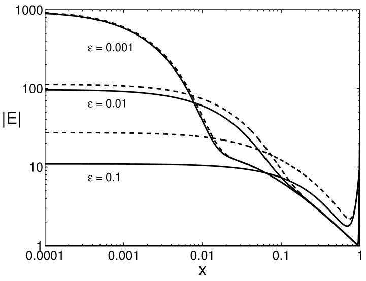
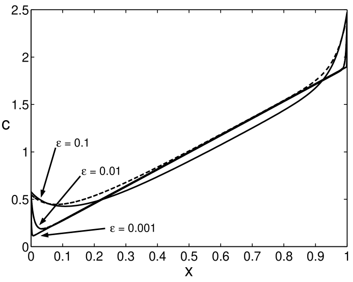
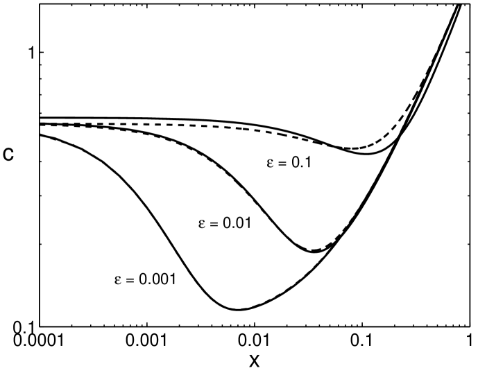
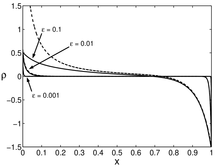
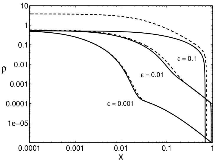
Fig. 1: Numerical solutions (solid lines) compared with the leading order uniformly-valid approximations (dashed lines) given by Eq. (58)-(61) for the dimensionless potential, $\phi(x)$, electric field, $E(x)$, concentration, $c(x)$, and charge density, $\rho(x)$ for the case $j=0.9$, $k_{c}=10$, $j_{r}=10$, $\delta=0$, and $\epsilon=0.001,0.01,0.1$. Linear scales on the left show the entire cell, while log scales on the left zoom in on the cathodic region. Note that in the concentration and charge density profiles, the numerical and asymptotic solutions are barely distinguishable for $\epsilon\leq 0.01$.

2.1 Electroneutrality in the Bulk Solution

The most fundamental approximation in electrochemistry is that of bulk electroneutrality [1]. As first emphasized by Newman [21], however, this does not mean that the charge density is vanishing or unimportant, but rather that over macroscopic distances the charge density is small compared to the total concentration, $|C_{+}-C_{-}|\ll C_{+}+C_{-}$, or, in our dimensionless notation, $|\rho|\ll c$. Mathematically, the “macroscopic limit” corresponds to the limit $\epsilon=\lambda_{D}/L\rightarrow 0$. The electroneutral solution is just the leading order solution when asymptotic series of the form $f(x)=f^{(0)}(x)+\epsilon f^{(1)}(x)+\epsilon^{2}f^{(2)}(x)+\ldots$, are substituted for the field variables in Eqs. (24)-(26).

Carrying out these substitutions and collecting terms with like powers of $\epsilon$, we obtain a hierarchy of differential equations for the expansion functions. At $O(1)$ we have,

$$\frac{d\bar{c}^{(0)}}{dx}=2j\ \ ,\ \ -\bar{c}^{(0)}\bar{E}^{(0)}=2j\ \ ,\ \ \bar{\rho}^{(0)}=0$$ (34)

where the bar accent indicates that these expansions are valid in the “bulk region” $\epsilon\ll x\ll 1-\epsilon$ (or $\lambda_{D}\ll X\ll L-\lambda_{D}$). Integating these equations, we obtain the leading order bulk solution:

$$\bar{c}^{(0)}(x) = c_{o}+2jx$$ (35)

$${\bar{E}}^{(0)}(x) = \frac{-1}{x+c_{o}/2j}$$ (36)

$${\bar{\phi}}^{(0)}(x) = \phi_{o}+\log\left(1+\frac{2jx}{c_{o}}\right)$$ (37)

where the constants of integration $c_{o}$ and $\phi_{o}$ are the values of the bulk concentration and potential extrapolated to the cathode surface at $x=0$. Note that, despite quasi-electroneutrality, the electrostatic potential does not satisfy Laplace’s equation at leading order in the bulk, as emphasized by Levich [46] and Newman [1]. Noting the presence of $\epsilon^{2}$ in Eq. (26) for the dimensionless potential, it is clear that a negligible charge density, $\rho=O(\epsilon^{2})$, is perfectly consistent with a nonvanishing Laplacian of the potential. More precisely, we have,

$${\bar{\rho}}^{(2)}(x)=\frac{d^{2}{\bar{\phi}}^{(0)}}{dx^{2}}(x)=\frac{1}{(x+c_{o}/2j)^{2}},$$ (38)

at $O(\epsilon^{2})$ in Eq. (26).

The integral constaint, Eq. (31), can be used to evaluate the constant $c_{o}$. If we assume that $c_{-}$ in the boundary layers does not diverge as $\epsilon\rightarrow 0$, then they only contribute $O(\epsilon)$ to the total anion number. Therefore,

$$1=\int_{0}^{1}c_{-}(x)dx=\int_{0}^{1}\bar{c}^{(0)}(x)dx+O(\epsilon)=c_{o}+j+O(\epsilon),$$ (39)

which implies that $c_{o}=1-j$.

At leading order in the bulk, we have recovered the classical theory dating back a century to Nernst [12, 13, 14]. The solution is electrically neutral with a linear concentration profile whose slope is proportional to the current. This approximation leads to one of the fundamental concepts in electrochemistry, that there exists a “limiting current”, $j=1$, or

$$I=I_{d}=\frac{4zFD_{+}C_{ref}A}{L},$$ (40)

corresponding to zero concentration at the cathode, $c_{o}=1-j=0$. The current is limited by the maximum rate of mass transfer allowed by diffusion, and larger currents would lead to unphysical and mathematically inconsistent negative concentrations (see Appendix A).

Examination of the electric field exposes the same limitation on the current: a singularity exists at $j=1$ that blocks larger currents from being attained. The leading order bulk approximation to the electric field, $\bar{E}^{(0)}=1/[x+(1-j)/2j]$, diverges near the cathode like $1/x$ in the limit $j\rightarrow 1$. This would imply that the cell voltage $v$ (calculated below) diverges as $j\rightarrow 1$, thus providing a satisfactory theory of the limiting current since an infinite voltage would be necessary to exceed (or even attain) it. Unfortunately, this classical picture due to Nernst [12], based on passing to the singular limit $\epsilon=0$, is not valid for any finite value of $\epsilon$ because the solution is, in general, unable to satisfy all of the boundary conditions.

2.2 Diffuse Charge Layers in Thermal Equilibrium

We now derive the leading order description of the boundary layers in the standard way [21, 5, 26, 1], using Eqs. (24)–(25). The singular perturbation in Eq. (26) can be eliminated with the rescaling $y=x/\epsilon$ indicating that the boundary layer at $x=0$ has a width $O(\epsilon)$. In terms of this inner variable, the governing equations in the cathode boundary layer are

$$\frac{dc}{dy}+\rho\frac{d\phi}{dy} = 2j\epsilon$$ (41)

$$\frac{d\rho}{dy}+c\frac{d\phi}{dy} = 2j\epsilon$$ (42)

$$-\frac{d^{2}\phi}{dy^{2}} = \rho,$$ (43)

where $\epsilon$ now appears as a regular perturbation since solutions satisfying the cathode boundary conditions and the matching conditions still exist when $\epsilon=0$. At the anode, the appropriate inner variable is $y=(1-x)/\epsilon$, and the equations are the same as above except that $j$ is replaced with $-j$, since current is leaving the anode layer, while it entering the cathode boundary layer.

Expanding the cathode boundary layer fields (indicated by the check accent) as asymptotic series in powers of $\epsilon$, we obtain at leading order,

$$\frac{d\check{c}^{(0)}}{dy}+{\check{\rho}}^{(0)}\frac{d{\check{\phi}}^{(0)}}{dy}=0$$ (44)

$$\frac{d{\check{\rho}}^{(0)}}{dy}+\check{c}^{(0)}\frac{d{\check{\phi}}^{(0)}}{dy}=0.$$ (45)

Using Eq. (23) to rewrite these equations in terms of $c_{+}$ and $c_{-}$, we find that the flux of each ionic species in the boundary layer is zero at leading order:

$$\frac{d\check{c}_{\pm}^{(0)}}{dy}\pm\check{c}_{\pm}^{(0)}\frac{d{\check{\phi}}^{(0)}}{dy}=0,.$$ (46)

While this equation appears to contradict the fact that the current is nonzero, the paradox is resolved in the same way as electroneutrality is reconciled with a non-harmonic potential in the bulk region: tiny fluctuations about the boundary layer equilibrium concentration profiles at $O(\epsilon)$ are amplified by a scaling factor of $1/\epsilon$ to sustain the $O(1)$ current. Thus, the leading order contribution to the current in the boundary layer is

$$\epsilon\left(\frac{d\check{c}_{+}^{(1)}}{dx}+\check{c}_{+}^{(1)}\frac{d{\check{\phi}}^{(0)}}{dx}+\check{c}_{+}^{(0)}\frac{d{\check{\phi}}^{(1)}}{dx}\right)=\frac{d\check{c}_{+}^{(1)}}{dy}+\check{c}_{+}^{(1)}\frac{d{\check{\phi}}^{(0)}}{dy}+\check{c}_{+}^{(0)}\frac{d{\check{\phi}}^{(1)}}{dy}=4j.$$ (47)

Integrating Eq. (46) and matching with the bulk, we find that the leading order ionic concentrations are Boltzmann equilibrium distributions:

$$\check{c}_{\pm}^{(0)}(y)=c_{o}e^{\pm[\phi_{o}-{\check{\phi}}^{(0)}(y)]}$$ (48)

where $c_{o}=1-j$ and $\phi_{o}={\bar{\phi}}^{(0)}(0)$ are obtained by matching with the solution in the bulk. Note that the Boltzmann distribution arises not from an assumption of thermal equilibrium in the boundary layer but as the leading order concentration distribution, even in the presence of a non-negligible $O(1)$ current.

The general leading-order solution was first derived by Gouy [42] and Chapman [43] and appears in numerous books [1, 26, 32, 33] and recent papers [5, 19]:

$$\check{c}^{(0)}(y) = c_{o}\cosh[\phi_{o}-{\check{\phi}}^{(0)}(y)]$$ (49)

$${\check{\rho}}^{(0)}(y) = c_{o}\sinh[\phi_{o}-{\check{\phi}}^{(0)}(y)]$$ (50)

$$\frac{d{\check{\phi}}^{(0)}}{dy} = 2\sqrt{c_{o}}\sinh\left(\frac{\phi_{o}-{\check{\phi}}^{(0)}(y)}{2}\right)$$ (51)

$${\check{\phi}}^{(0)}(y) = \phi_{o}+4\tanh^{-1}\left(\gamma_{o}e^{-\sqrt{c_{o}}y}\right),$$ (52)

where $\gamma_{o}\equiv\tanh(\zeta_{o}/4)$ and $\zeta_{o}\equiv{\check{\phi}}^{(0)}(0)-\phi_{o}$ is the leading order “zeta potential” across the cathodic diffuse layer, which plays a central role in electrokinetic phenomena [32, 33]. Note that the magnitude of the diffuse layer electric field scales as $1/\epsilon$ as illustrated in Figure 1.

The value of ${\check{\phi}}^{(0)}(0)$ hidden in the zeta potential $\zeta_{o}$ is determined by the Stern boundary condition, Eq. (27). If $\delta=0$ (Gouy-Chapman model), then ${\check{\phi}}^{(0)}(0)=0$, or $\zeta_{o}=-\phi_{o}$, which means that the entire voltage drop $\phi_{o}$ across the cathodic double layer occurs in the diffuse layer. If $\delta=\infty$ (Helmholtz model), then ${\check{\phi}}^{(0)}(0)=\phi_{o}$, or $\zeta_{o}=0$, in which case the Stern layer carries all the double layer voltage. For finite $\delta>0$ (Stern model), $\zeta_{o}$ is obtained in terms of $\phi_{o}$ by solving a trancendental algebraic equation,

$$-\zeta_{o}=2\delta\sqrt{c_{o}}\sinh(\zeta_{o}/2)+\phi_{o},$$ (53)

which can be linearized about the two limiting cases and solved for $\zeta_{o}$,

$$-\zeta_{o}\sim\left\{\begin{array}[]{ll}\phi_{o}-2\delta\sqrt{c_{o}}\sinh(\phi_{o}/2)&\mbox{ if }\delta\ll\phi_{o}/2\sqrt{c_{o}}\sinh(\phi_{o}/2)\\ \phi_{o}/\delta\sqrt{c_{o}}&\mbox{ if }\delta\gg\phi_{o}/2\sqrt{c_{o}}\end{array}\right.$$ (54)

Note that if $\phi_{o}\ll 1$, then $-\zeta_{o}\approx\frac{\phi_{o}}{1+\delta\sqrt{c_{o}}}$ is a reasonable approximation for any value of $\delta\geq 0$. Finally, we solve for $\phi_{o}$ by applying the Butler-Volmer rate equation, Eq. (29), which yields a transcendental algebraic equation for $\phi_{o}$:

$$k_{c}c_{o}e^{-\zeta_{o}+\alpha_{c}(\zeta_{o}+\phi_{o})}-j_{r}e^{-\alpha_{a}(\zeta_{o}+\phi_{o})}=j.$$ (55)

Simultaneously solving the pair of equations (53) and (55) exactly is not possible in general, but below we will analyze various limiting cases.

In the anodic boundary layer, we find the same set of equations as Eqs. (41)-(43) except that $j$ is replaced by $-j$. Therefore, since the fields do not depend on $j$ at leading order, the anodic boundary layer has the same structure but with different constants of integration. Thus, we find that the leading order description of the anodic boundary layer is given by Eqs (49)-(52) with $c_{o}$, $\phi_{o}$, $\gamma_{o}$, and $\zeta_{o}$ replaced by different constants $c_{1}$, $\phi_{1}$, $\gamma_{1}$, and $\zeta_{1}$, respectively. Moreover, it is straightforward to show that $c_{1}=\bar{c}^{(0)}(1)=1+j$ and $\phi_{1}=\phi_{o}+\log\left(\frac{1+j}{1-j}\right)$.

The leading-order anodic zeta potential, $\zeta_{1}$, and potential drop across the entire anodic double layer, $v-\phi_{1}$, are found by solving another pair of trancendental algebraic equation resulting from the anode Stern and Butler-Volmer boundary conditions, Eqs. (28) and (30),

$$-\zeta_{1} = 2\delta\sqrt{c_{1}}\sinh(\zeta_{1}/2)+\phi_{1}-v$$ (56)

$$j = -k_{c}c_{1}e^{-\zeta_{1}+\alpha_{c}(\zeta_{1}+\phi_{1}-v)}+j_{r}e^{-\alpha_{a}(\zeta_{1}+\phi_{1}-v)}.$$ (57)

As before, the Gouy-Chapman and Helmholtz limits are $\zeta_{1}=v-\phi_{1}$ and $\zeta_{1}=0$, respectively, and for small voltages (or currents) the approximation $\zeta_{1}\approx(v-\phi_{1})/(1+\delta\sqrt{c_{1}})$ is valid for all $\delta\geq 0$.

2.3 Leading Order Uniformly-valid Approximations

We obtain asymptotic approximations that are uniformly valid across the cell by adding the bulk and boundary layer approximations and subtracting the overlapping parts:

$$c(x) = [\check{c}^{(0)}(x/\epsilon)-c_{o}]+\bar{c}^{(0)}(x)+[\hat{c}^{(0)}((1-x)/\epsilon)-c_{1}]+O(\epsilon),$$ (58)

$$\rho(x) = {\check{\rho}}^{(0)}(x/\epsilon)+\epsilon^{2}{\bar{\rho}}^{(2)}(x)+{\hat{\rho}}^{(0)}((1-x)/\epsilon)+O(\epsilon),$$ (59)

$$E(x) = \frac{1}{\epsilon}\frac{d{\check{\phi}}^{(0)}}{dy}(x/\epsilon)+\frac{d{\bar{\phi}}^{(0)}}{dx}(x)-\frac{1}{\epsilon}\frac{d{\hat{\phi}}^{(0)}}{dy}((1-x)/\epsilon)+O(\epsilon),$$ (60)

$$\phi(x) = [{\check{\phi}}^{(0)}(x/\epsilon)-\phi_{o}]+{\bar{\phi}}^{(0)}(x)+[{\hat{\phi}}^{(0)}((1-x)/\epsilon)-\phi_{1}]+O(\epsilon).$$ (61)

Note that we have kept the $O(\epsilon^{2})$ term in the charge density since it is the leading order contribution in the bulk region and is easily computed from Eq. (38). As shown in Figure 1, the leading-order uniformly valid solutions are very accurate for $\epsilon\leq 0.01$ (or $L\geq 100\lambda_{D}$) and reasonably good for $\epsilon=0.1$. Since higher-order terms are not analytically tractable, it seems numerical solutions must suffice for nanolayers, where $\epsilon\approx 1$, or else other limits of various parameters must be considered, as below.

The discrepancy in electric potential profile at large $\epsilon$ in Figure 1 is particularly interesting because it arises from a constraint on the total potential drop across the cell. To understand the origin of this voltage constraint, recall that the total cell voltage is determined by the current density flowing through the cell (via the voltage-current relationship). While $\epsilon$ is technically a parameter in the voltage-current relationship, a leading-order analysis does not capture the $\epsilon$ dependence. Thus, the leading-order cell voltage must be the same for all $\epsilon$ which is what we observe in figure 1. A close examination of the potential and electric field profiles reveals that most of the error in the asymptotic solution for the potential comes from an over prediction of the electric field strength (and therefore the potential drop) in cathode region.

3 Polarographic Curves for Thin Double Layers, $\epsilon\rightarrow 0$

The relationship between current and cell voltage is of primary importance in the study of any electrochemical system, so we now use the results from the previous section to calculate theoretical polarographic curves in several physically relevant regimes. We focus on the effects of the Stern capacitance and the reaction rate constants through the dimensionless parameters, $\delta$, $k_{c}$ and $j_{r}$, with $\alpha_{c}=\alpha_{a}=1/2$. For a fixed voltage, the mathematical results are valid in the asymptotic limit of thin double layers, $\epsilon\rightarrow 0$.

3.1 Exact Results at Leading Order

Using the uniformly valid approximation Eq. (61), we can write the leading order approximation for the cell voltage as

$$v=\phi_{o}+2\tanh^{-1}(j)+(v-\phi_{1}).$$ (62)

We can interpret this expression as a decomposition of the cell voltage into the potential drop across the cathode, bulk, and anode layers respectively. Note the divergence in the bulk contribution to the cell voltage as $j\rightarrow 1$, which we expect from our earlier analysis. In the next section, we explore analytic solutions for several limiting cases and compare them to exact solutions given by Eq. (62) with the leading-order cathode and anode diffuse layer potential drops determined implicitly by Eqns. (53), (55), (56). To make plots in our figures, we use Newton iteration to solve for $\phi_{o}$ and $v-\phi_{1}$ in this algebraic system.

3.2 Cell Resistance at Low Current

Given the common practice of using linear circuit models to describe electrochemical systems [27, 28, 20], it is important to consider the low-current regime, where the cell acts as a simple resistance, $R=V/I$. First, we compute the potential drop across the double layers. Since the procedure is almost identical for the two boundary layers, we focus on the calculation for the cathode. By writing the boundary conditions Eq. (29) in the standard Butler-Volmer form involving the exchange current and surface overpotential [26, 1]:

$$j=j_{o}^{c}\left(e^{-\alpha_{c}\eta_{s}^{c}}-e^{\alpha_{a}\eta_{s}^{c}}\right)$$ (63)

where $j_{o}^{c}=\left(k_{c}c_{o}e^{-\zeta_{o}}\right)^{\alpha_{a}}j_{r}^{\alpha_{c}}$ and $\eta_{s}^{c}=\Delta\phi_{S}-\Delta\phi_{S}^{eq}$ are the cathode exchange current and surface overpotential, respectively. Note that the exchange current contains the Frumkin correction through the factor $e^{-\zeta_{o}}$ [26]. For low current densities, we expect the surface overpotential to be small, so we can linearize this equation to obtain

$$j\sim-j_{o}^{c}\eta_{s}^{c}$$ (64)

where we have used the fact that $\alpha_{c}+\alpha_{a}=1$. Rewriting this equation in terms of ${\check{\phi}}(0)$, we find that

$${\check{\phi}}(0)\sim\frac{j}{j_{o}^{c}}+{\check{\phi}}_{eq}(0),$$ (65)

where ${\check{\phi}}_{eq}(0)$ is the value of ${\check{\phi}}(0)$ calculated from the cathode Butler-Volmer rate equation when there is no current flowing through the electrode. The zeta potential $\zeta_{o}$ in the formula for the exchange current is determined by combining Eq. (65) with (53) to obtain a single equation for $\zeta_{o}$:

$$-2\delta\sqrt{c_{o}}\sinh\left(\zeta_{o}/2\right)\sim\frac{j}{\left(k_{c}c_{o}e^{-\zeta_{o}}\right)^{\alpha_{a}}j_{r}^{\alpha_{c}}}+\log\left(\frac{j_{r}}{k_{c}c_{o}}\right)+\zeta_{o}.$$ (66)

Finally, to compute the total double layer potential drop we add the potential drop across the diffuse layer to ${\check{\phi}}(0)$:

$$\phi_{o}={\check{\phi}}(0)-\zeta_{o}\sim\frac{j}{j_{o}^{c}}+\log\left(\frac{j_{r}}{k_{c}c_{o}}\right).$$ (67)

A similar calculation at the anode results in

$$v-\phi_{1}\sim\frac{j}{j_{o}^{a}}+\log\left(\frac{k_{c}c_{1}}{j_{r}}\right),$$ (68)

where $j_{o}^{a}=\left(k_{c}c_{1}e^{-\zeta_{1}}\right)^{\alpha_{a}}j_{r}^{\alpha_{c}}$ and $\zeta_{1}$ is determined by the anode equivalent of Eq. (66).

Combining these results with the potential drop across the bulk solution, we find that the total cell voltage is given by

$$v(j) \sim 4\tanh^{-1}(j)+\frac{j}{j_{o}^{c}}+\frac{j}{j_{o}^{a}}$$

$$\approx j\left(4+\frac{1}{j_{o}^{c}}+\frac{1}{j_{o}^{a}}\right).$$

$$= j\;r$$

This result gives the dimensionless resistance, $r$, of the electrochemical thin film as a function of the physical properties of the electrodes and the electrolyte. Note that the Stern-layer capacitance is accounted for implicitly via the calculation of the electrode zeta potentials.

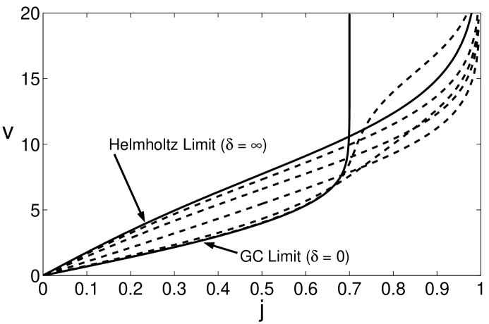
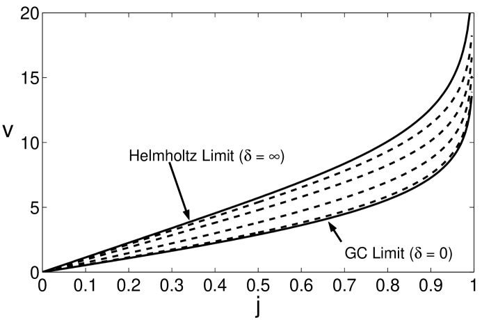
Fig. 2: Exact polarographic curves (dashed lines) for varying $\delta$ values compared to polarographic curves for the Gouy-Chapman ($\delta=0$) and Helmholtz ($\delta=\infty$) limits (solid lines). Top: a reaction-limited cell ($j_{r}<1$) with physical parameters, $k_{c}=0.03,j_{r}=0.7$. Notice that above the reaction-limited current density, $j_{r}$, the highest cell voltages occur for $\delta$ values near $0$. Bottom: a diffusion-limited cell ($j_{r}>1$) with physical parameters: $k_{c}=0.05,j_{r}=1.5$. In both cases, $\delta$ increases as the curves move upwards.

3.3 Simple Analytical Formulae

The exact leading-order current-voltage relation simplifies considerably in a variety of physically relevant limits. These approximate formulae provide insight into the basic physics and may be useful in interpretting experimental data.

3.3.1 The Gouy-Chapman Limit $(\delta\rightarrow 0)$

In this limit, the capacitance of the diffuse layer of the charged double layer is negligible compared to the capacitance of the compact layer. As a result, the voltage drop across the diffuse layer accounts for the entire potential drop across the charged double layer. Physically, this limit corresponds to the limits of low ionic concentration or zero ionic volume [26]. Since $\zeta_{o}=-\phi_{o}$ and $\zeta_{1}=v-\phi_{1}$ when $\delta=0$, the Butler-Volmer rate equations, Eqs. (55) and (57), reduce to

$$k_{c}(1-j)e^{-\zeta_{o}}-j_{r}=j\ \ \textrm{and}\ \ -k_{c}(1+j)e^{-\zeta_{1}}+j_{r}=j.$$ (70)

Solving for $\zeta_{o}$ and $\zeta_{1}$, we find that

$$\zeta_{o}=\ln\left(1-j\right)-\ln\left(\frac{j_{r}+j}{k_{c}}\right)\ \ \textrm{and}\ \ \zeta_{1}=\ln\left(1+j\right)+\ln\left(\frac{k_{c}}{j_{r}-j}\right),$$ (71)

which can be substituted into Eq. (62) to obtain

$$v(j)=4\tanh^{-1}(j)+2\tanh^{-1}(j/j_{r}).$$ (72)

Notice that the boundary layers make a nontrivial contribution to the leading order cell voltage. The $2\tanh^{-1}(j/j_{r})$ term is especially interesting because it indicates the existence of a reaction-limited current when $j_{r}<1$. In hindsight, it is obvious that reaction limited currents exist in the Gouy-Chapman limit because the reaction kinetics at the anode do not permit a current greater than $j_{r}$. We emphasize, however, that the Gouy-Chapman limit is singular because there is no problem achieving current densities above $j_{r}$ for any $\delta>0$ (see Figure 2). For any finite $\delta>0$, the shift of the anode double-layer potential drop to the Stern layer helps the dissolution reaction while suppressing the deposition reaction which permits the current density to rise greater than $j_{r}$.

Note that the cathodic and anodic boundary layers do not evenly contribute to the cell voltage near the limiting currents. In a diffusion-limited cell, the cathodic layer makes the greater contribution because as $j\rightarrow 1$, $\zeta_{o}$ diverges while $\zeta_{1}$ approaches a finite limit. We expect this behavior because as $j\rightarrow 1$, the electric field only diverges at $x=0$. However, when the cell is reaction-limited, the division of cell voltage between the boundary layers is reversed as $j$ approaches the limiting current $j_{r}$. Even the voltage drop in the bulk becomes negligible compared to $\zeta_{1}$ in the reaction-limited case. In this situation, the cell voltage diverges as $j\rightarrow j_{r}$ because the only way to achieve a current near $j_{r}$ is to drastically reduce the deposition reaction at the anode. In other words, the cation concentration at the anode must be made extremely small which requires a huge anodic zeta potential.

3.3.2 The Helmholtz Limit $(\delta\rightarrow\infty)$

This is the reverse of the Gouy-Chapman limit. Here, the capacitance of the compact layer is negligible, so the potential drop across the double layer resides completely in the compact layer. The Helmholtz limit holds for concentrated solutions or solvents with low dielectric constants and other situations where the Debye screening length becomes negligible [26]. It also describes a thick dielectric or insulating layer on an electrode [38, 20].

In the Helmholtz limit, $\zeta_{o}=0=\zeta_{1}$, so the Butler-Volmer rate equations take the form

$$k_{c}(1-j)e^{\alpha_{c}\phi_{o}}-j_{r}e^{-\alpha_{a}\phi_{o}} = j$$ (73)

$$-k_{c}(1+j)e^{\alpha_{c}(\phi_{1}-v)}+j_{r}e^{-\alpha_{a}(\phi_{1}-v)} = j.$$ (74)

Solving these equations for $\phi_{o}$ and $v-\phi_{1}$ under the assumption of a symmetric electron-transfer reaction (i.e. $\alpha_{c}=1/2=\alpha_{a}$) and substituting into the formula for the cell voltage, we find that

$$v(j)=6\tanh^{-1}(j)+2\ln\left(\frac{j+\sqrt{j^{2}+4j_{r}k_{c}(1-j)}}{-j+\sqrt{j^{2}+4j_{r}k_{c}(1+j)}}\right).$$ (75)

While this expression appears to be more complicated than the one obtained for the Gouy-Chapman model, it is not very different when $j_{r}>1$ as can be seen in Figures 2 and 3. In fact, the wide spread in the polarographic curves observed in Figure 2 requires that $k_{c}\ll j_{r}$; otherwise, all of the curves would be difficult to distinguish. Moreover, as we shall see in the next section, in limit of fast reactions, both models lead to the same expression for the cell voltage for $j_{r}>1$. On the other hand, when $j_{r}<1$, the two models are qualitatively very different. While the Gouy-Chapman model gives rise to a reaction-limited current, the Helmholtz model does not.

3.3.3 The Fast-Reaction Limit, $(j_{r}\gg 1,(j_{r})^{\alpha_{a}}(k_{c})^{\alpha_{c}}\gg j/(1-j)^{\alpha_{a}})$

The polarographic curves for all $\delta$ values collapse onto each other in the limit of fast reaction kinetics (Figure 3). Even the assumption of symmetry in the electron-transfer reaction is not required. When reaction rates are much larger than the current, the two reaction-rate terms in the Butler-Volmer equations, Eqs. (55) and (57), must balance each other at leading order:

$$k_{c}(1-j)e^{-\zeta_{o}+\alpha_{c}(\zeta_{o}+\phi_{o})}-j_{r}e^{-\alpha_{a}(\zeta_{o}+\phi_{o})} \approx 0$$ (76)

$$-k_{c}(1+j)e^{-\zeta_{1}+\alpha_{c}(\zeta_{1}+\phi_{1}-v)}+j_{r}e^{-\alpha_{a}(\zeta_{1}+\phi_{1}-v)} \approx 0.$$ (77)

Since $\alpha_{c}+\alpha_{a}=1$ for theoretical models of single electron-transfer reactions [1, 11, 29], we can solve explicitly for $\phi_{o}$ and $v-\phi_{1}$ to obtain

$$\phi_{o}=\ln\left(\frac{j_{r}}{k_{c}(1-j)}\right)\ \ \ ,\ \ \ v-\phi_{1}=\ln\left(\frac{k_{c}(1+j)}{j_{r}}\right).$$ (78)

Thus, for fast reaction kinetics, the leading order cell voltage is given by

$$v(j)=4\tanh^{-1}(j).$$ (79)

Notice that this is exactly the fast reaction limit of $v(j)$ that we find in both the Gouy-Chapman and Helmholtz limits. It is straightforward to check the validity of the assumptions made in Eqs. (76) and (77) by substituting these results into the expresssions for the reaction rates and observing that the zeta potentials satisfy the bounds $\zeta_{o}\leq 0$ and $\zeta_{1}\leq\ln\left(\frac{k_{c}(1+j)}{j_{r}-j}\right)$ which follow from the monotonicity of $\zeta_{o}$ and $\zeta_{1}$ as functions of $\delta$.

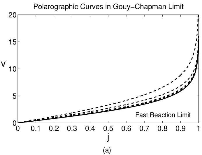
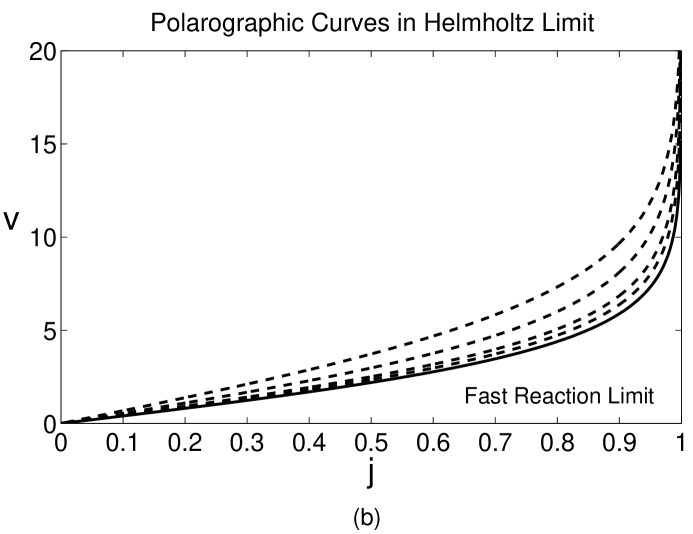
Fig. 3: Polarographic curves in the (a) Gouy-Chapman limit and (b) Helmholtz limit as the reaction rate constants are increased (dashed lines). For these plots, the reaction rate constants ($j_{r}=1,2,5,and10$) increase as the curves shift towards the lower right and are related by $k_{c}=j_{r}/2$. It should be noted that the fast reaction limit is reached very quickly; in both plots, the curve closest to the fast reaction curve has a $j_{r}$ value of only $10$.

4 Thick Double Layers, $\epsilon=O(1)$

Up to this point, we have only examined the current-voltage characteristics in the singular limit $\epsilon\rightarrow 0$, where the current density cannot exceed its diffusion-limited value, $j=1$. The situation changes changes for any finite $\epsilon>0$.

4.1 What Limiting Current?

As is clearly evident in Figure 4, the cell has no problem breaking through the classical limiting current for $\epsilon>0$. Figure 4 also shows that the $\epsilon$ dependence of the polarographic curves only becomes significant at currents approaching the diffusion-limited current; below $j\approx 0.5$, the curves are nearly indistinguishable. Moreover, as $\epsilon$ increases, upper end of the polarographic curves flatten out and shift downwards. This decrease in the cell voltage for large $\epsilon$ values arises because the diffuse charge layers overlap and are able to interact with each other. More precisely, the cell has become so small (relative to the Debye screening length) that the electric fields from the two diffuse layers partially cancel each other out throughout the cell resulting in a lower total cell voltage. It should be emphasized that this effect is only observable because we are studying a two electrode system. Single electrode systems (in addition to being not physically achievable) are not capable of showing this behavior because they always implicitly assume an infinite system size which effectively discards any interactions from “far away” electrodes.

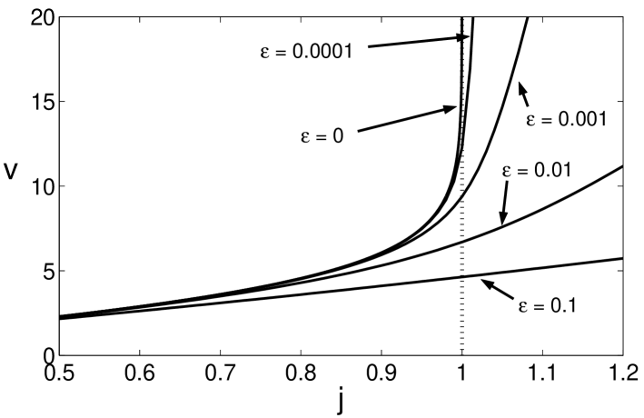
Fig. 4: Polarographic curves for $\epsilon$ values of $0$, $0.0001$, $0.001$, $0.01$, and $0.1$ (listed in order from uppermost to lowest curves) with the other physical parameters taken to be $\delta=0$, $k_{c}=10$, and $j_{r}=10$. Notice that for any $\epsilon>0$, the cell has no problem achieving current densities higher than the diffusion limited current (dashed vertical line). All of these curves, with the exception of the exact $\epsilon=0$ curve, were generated by numerically solving Eq. (24)-(26) subject to the boundary conditions (27)-(31) using the method of our companion paper[22].

4.2 Breakdown of the Classical Approximation

For a diffusion-limited cell, the classical nonlinear asymptotic analysis just presented leads to an aesthetically appealing theory that predicts a limiting current at $j=1$. The existence of this limiting current fits nicely with our physical intuition that the concentration of cations in a solution must always remain nonnegative. In reality, however, the analysis breaks down as the current approaches (and exceeds) its limiting value.

The breakdown of the classical asymptotics is evident upon examining the expansions for the bulk field variables as the current is increased toward its diffusion-limited value. Calculating a few of the higher order terms in the bulk asymptotic expansion, we find that

$$-{\bar{E}}(x) = \frac{2j}{\bar{c}^{(0)}}+\frac{3}{2}\epsilon^{2}\frac{(2j)^{3}}{\left(\bar{c}^{(0)}\right)^{4}}+\frac{111}{4}\epsilon^{4}\frac{(2j)^{5}}{\left(\bar{c}^{(0)}\right)^{7}}+\frac{6045}{4}\epsilon^{6}\frac{(2j)^{7}}{\left(\bar{c}^{(0)}\right)^{10}}+O(\epsilon^{8})$$ (80)

$$\bar{c}(x) = \bar{c}^{(0)}+\frac{1}{2}\epsilon^{2}\frac{(2j)^{2}}{\left(\bar{c}^{(0)}\right)^{2}}+\frac{3}{2}\epsilon^{4}\frac{(2j)^{4}}{\left(\bar{c}^{(0)}\right)^{5}}+\frac{231}{8}\epsilon^{6}\frac{(2j)^{6}}{\left(\bar{c}^{(0)}\right)^{8}}+O(\epsilon^{8})$$ (81)

$${\bar{\rho}}(x) = 0+\epsilon^{2}\frac{(2j)^{2}}{\left(\bar{c}^{(0)}\right)^{2}}+6\epsilon^{4}\frac{(2j)^{4}}{\left(\bar{c}^{(0)}\right)^{5}}+\frac{777}{4}\epsilon^{6}\frac{(2j)^{6}}{\left(\bar{c}^{(0)}\right)^{8}}+O(\epsilon^{8}).$$ (82)

Since $\bar{c}^{(0)}\rightarrow 2x$ as $j\rightarrow 1$, the higher order terms are clearly more singular than the leading order term at the limiting current. Rubinstein and Shtilman make a similar observation from a potentiostatic perspective; they note that the asymptotic expansions are not uniform in the cell voltage [24].

The inconsistency in the classical approximation was apparently first noticed by Levich who observed that the leading-order solution in the bulk predicts an infinite charge density when the current density reaches $1$, which directly contradicts the assumption of bulk charge neutrality [46]. As $j\rightarrow 1$, the bulk charge density is given by

$${\bar{\rho}}=-\epsilon^{2}\frac{d^{2}{\bar{\phi}}}{dx^{2}}=\frac{\epsilon^{2}}{\left[x+(1-j)/2j\right]^{2}}\approx\frac{\epsilon^{2}}{x^{2}},$$ (83)

which diverges at the cathode.

Smyrl and Newman first showed that these paradoxical results are related to the breakdown of thermal equilibrium charge profiles near the cathode, leading to a significant expansion of the double layer into the bulk solution [23]. They argue that the assumption of electroneutrality breaks down when ${\bar{\rho}}\approx\bar{c}$. Since $\bar{c}$ is proportional to $x$ at the limiting current, the bulk approximation fails to be valid for $x$ smaller than $O(\epsilon^{2/3})$, which leads to a boundary layer that is thicker than the usual Debye length. From an alternative perspective, the problems begin when ${\bar{\rho}}(0)/\bar{c}(0)\approx 1$ (see Figure 5). Using this criterion, we find that the classical asymptotic theory is only appropriate when $c_{o}\gg(2j\epsilon)^{2/3}$ or, equivalently, $j\ll 1-(2\epsilon)^{2/3}$. Since the cell voltage is approximately $4\tanh^{-1}(j)$ in many situations, this regime also corresponds to $v=O\left(|\ln\epsilon|\right)$. This shows that in thin films, where $\epsilon$ is not so small, it is easy to exceed the classical limiting current and achieve rather different charge profiles [22].

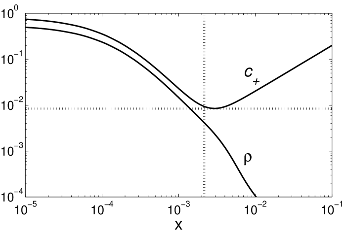
Fig. 5: Numerical solutions for the dimensionless cation concentration $c_{+}(x)$ and (full) charge density $2\rho(x)$ at the diffusion-limited current ($j=1.0$) with physical parameters $k_{c}=10$, $j_{r}=10$, $\alpha_{c}=\alpha_{a}=0.5$, $\delta=0.0$ and $\epsilon=0.0001$. In the cathode region, electroneutrality breaks down as the solution becomes cation rich in order to satisfy the reaction boundary conditions. Note that when $x=O(\epsilon^{2/3})$, $c_{+}$ and $\rho$ are both $O(\epsilon^{2/3})$. For reference, the dashed vertical line shows where $x=\epsilon^{2/3}$, and the dashed horizontal line shows where $y=\epsilon^{2/3}\left[(2+2^{2/3})+4/(2+2^{2/3})^{2}\right]\approx c_{+}(\epsilon^{2/3})$.

5 Conclusion

In summary, we have revisited the classical PNP equations, analyzing for the first time the effect of physically realistic boundary conditions for thin-film galvanic cells and other micro-electrochemical systems. In particular, we focus on the effect of Stern-layer capacitance and Faradaic reactions with Butler-Volmer kinetics. Such boundary conditions contain new physics, such as the possibility of a reaction-limited current due to the slow injection of ions at the anode. We also find that the Stern layer generally allows the cell to exceed limiting currents by carrying diverging portions of the cell voltage, which would otherwise end up in the diffuse part of the double layer. We have provided analytical formulae for current-voltage relations that should provide useful in characterizing the differential resistance of thin films, such as those used in on-chip micro-batteries. Here, we have focused on the classical nonlinear regime in which thin double layers remain in thermal equilibrium; the more exotic, non-equilibrium regime, which arises at and above the classical limiting current, is analyzed in the companion paper [22].

6 Acknowledgments

This work was supported in part by the MRSEC Program of the National Science Foundation under award number DMR 02-13282 and in part by the Department of Energy through the Computational Science Graduate Fellowship (CSGF) Program provided under grant number DE-FG02-97ER25308. The authors thank F. Argoul, J. J. Chae, H. A. Stone, and W. Y. Tam, for many helpful discussions.

Appendix A Positivity of Ion Concentrations

The positivity of the ion concentrations follows directly from the mathematical formulation of the problem. For the anion concentration, equations (22) can be integrated exactly using the integrating factor $e^{\phi}$ to yield

$$c_{-}(x)=Ae^{\phi(x)},$$ (84)

which implies that the sign of $c_{-}(x)$ is the same across the entire domain. Since the integral constraint (31) requires that $c_{-}(x)$ is positive somewhere in the domain, $c_{-}(x)$ must be positive everywhere in the domain.

For the cation concentration, we make use of the reaction boundary conditions. Integrating equation (21) with the integrating factor $e^{\phi}$, we obtain

$$c_{+}(x)=c_{+}(0)e^{\phi(0)-\phi(x)}+4je^{-\phi(x)}\int_{0}^{x}e^{\phi(y)}dy.$$ (85)

Clearly, the integral term is postive because $e^{\phi}$ is positive everywhere. Moreover, the reaction boundary condition (29) implies that $c_{+}(0)>0$ because both $j_{r}$ and $k_{c}$ are positive. Thus, we find that the cation concentration is strictly positive.

References

- [1] J. Newman, Electrochemical Systems, Prentice-Hall, Inc., Englewood Cliffs, NJ, 1991.
- [2] I. Rubinstein, Electro-Diffusion of Ions, SIAM Studies in Applied Mathematics, SIAM, Philadelphia, PA, 1990.
- [3] V. Barcilon, D.-P. Chen, R. S. Eisenberg, Ion Flow Through Narrow Membrane Channels: Part II, SIAM J. Appl. Math, 52 (1992), pp. 1405–1425.
- [4] J.-H. Park and J. W. Jerome, Qualitative Properties of Steady-State Poisson-Nernst-Planck Systems: Mathematical Study, SIAM J. Appl. Math, 57 (1997), pp. 609–630.
- [5] V. Barcilon, D.-P. Chen, R. S. Eisenberg, and J. W. Jerome, Qualitative Properties of Steady-State Poisson-Nernst-Planck Systems: Perturbation and Simulation Study, SIAM J. Appl. Math, 57 (1997), pp. 631–648.
- [6] . N. J. Dudney, J. B. Bates, D. Lubben, and F. X. Hart, Thin-Film Rechargeable Lithium Batteries with Amorphous LixMn2O4 cathodes, in Thin Film Solid Ionic Devices and Materials, J. Bates, The Electrochemical Society, Pennington, NJ, 1995, pp. 201-214.
- [7] . B. Wang, J. B. Bates, F. X. Hart, B. C. Sales, R. A. Zuhr, and J. D. Robertson, Characterization of Thin-Film Rechargeable Lithium Batteries with Lithium Cobalt Oxide Cathodes, J. Electrochem. Soc., 143 (1996), pp. 3204-3213.
- [8] B. J. Neudecker, N. J. Dudney, J. B. Bates, “Lithium-Free” Thin-Film Battery with In Situ Plated Li Anode, J. Electrochem. Soc., 147 (2000), pp. 517–523.
- [9] N. Takami, T. Ohsaki, H. Hasabe, and M. Yamamoto, Laminated Thin Li-Ion Batteries Using a Liquid Electrolyte, J. Electrochem. Soc., 149 (2002), pp. A9–A12.
- [10] Z. Shi, L. Lü, and G. Ceder, Solid State Thin Film Lithium Microbatteries, Singapore-MIT Alliance Technical Report: Advanced Materials for Micro- and Nano-Systems Collection, Jan. 2003. http://hdl.handle.net/1721.1/3672.
- [11] C. M. A. Brett and A. A. O. Brett, Electrochemistry. Principles, Methods, and Applications, Oxford Science Publications, Oxford, 1993.
- [12] W. Nernst, , Z. Phys. Chem., 47 (1904), pp. 52–55.
- [13] E. Brunner, , Z. Phys. Chem., 47 (1904), pp. 56–102.
- [14] , , Z. Phys. Chem., 58 (1907), pp. 1–126.
- [15] H.-C. Chang and G. Jaffé, Polarization in Electrolytic Solutions. Part I. Theory, J. Chem. Phys., 20 (1952), pp. 1071–1077.
- [16] G. Jaffé and C. Z. LeMay, On Polarization in Liquid Dielectrics, J. Chem. Phys., 21 (1953), pp. 920–928.
- [17] E. M. Itskovich, A. A. Kornyshev, and M. A. Vorotyntsev, Electric Current across the Metal-Solid Electrolyte Interface. I. Direct Current, Current-Voltage Characteristic, phys. stat. sol. (a), 39 (1977), pp. 229–238.
- [18] A. A. Kornyshev and M. A. Vorotyntsev, Conductivity and Space Charge Phenomena in Solid Electrolytes with One Mobile Charge Carrier Species, A Review with Original Material, Electrochimica Acta, 26 (1981), pp. 303–323.
- [19] A. Bonnefont, F. Argoul, and M. Z. Bazant, Analysis of diffuse-layer effects on time-dependent interfacial kinetics, J. Electroanal. Chem., 500 (2001), pp. 52–61.
- [20] M. Z. Bazant, K. Thornton, and A. Ajdari, Diffuse-charge dynamics in electrochemical systems, to appear in Phys. Rev. E (2004).
- [21] J. Newman, The Polarized Diffuse Double Layer, Trans. Faraday Soc., 61 (1965), pp. 2229–2237.
- [22] K. T. Chu and M. Z. Bazant, Electrochemical thin films at and above the classical limiting current, preprint.
- [23] W. H. Smyrl and J. Newman, Double Layer Structure at the Limiting Current, Trans. Faraday Soc., 63 (1967), pp. 207–216.
- [24] I. Rubinstein and L. Shtilman, Voltage against Current Curves of Cation Exchange Membranes, J. Chem. Soc. Faraday. Trans. II, 75 (1979), pp. 231–246.
- [25] P. Delahay, Double Layer and Electrode Kinetics, Interscience Publishers, New York, NY, 1965.
- [26] A. J. Bard and L. R. Faulkner, Electrochemical Methods, John Wiley & Sons, Inc., New York, NY, 2001.
- [27] J. R. Macdonald, Electrochim. Acta, 35 (1990), p. 1483. GET FULL REF
- [28] L. A. Geddes, Historical evolution of circuit models for the electrode-electrolyte interface, Ann. Biomedical Eng., 25 (1997), pp. 1-14.
- [29] C. Chidsey, Kinetics of Electrode Reactions, in Physical Chemistry, R. S. Berry, S. A. Rice, J. Ross, Oxford University Press, New York, NY, 2000, pp. 999–1008.
- [30] O. Stern, Zur Theorie der Electrolytischen Doppelschicht, Z. Elektrochem., 30 (1924), pp. 508–516.
- [31] A. Frumkin, Wasserstoffüberspannung und Struktur der Doppelschict, Z. Phys. Chem., 164A (1933), pp. 121–133.
- [32] R. J. Hunter, Foundations of Colloid Science, Oxford University Press, Oxford, 2001.
- [33] J. Lyklema, Fundamentals of Interface and Colloid Science. Volume II: Solid-Liquid Interfaces, Academic Press Limited, San Diego, CA, 1995.
- [34] D. C. Grahame, The Electrical Double Layer and the Theory of Electrocapillarity, Chem. Rev., 41 (1947), pp. 441–501.
- [35] , Differential Capacity of Mercury in Aqueous Sodium Fluoride Solutions. I. Effect of Concentration at 25∘, J. Am. Chem. Soc., 76 (1954), pp. 4819–4823.
- [36] J. R. Macdonald, Theory of the Differential Capacitance of the Double Layer in Unadsorbed Electrolytes, J. Chem. Phys., 22 (1954), pp. 1857–1866.
- [37] J. R. Macdonald, Static Space Charge and Capacitance for a Single Blocking Electrode, J. Chem. Phys., 29 (1958), pp. 1346–1358.
- [38] A. Ajdari, AC pumping of liquids, Phys. Rev. E, 61 (2000), pp. R45–R48.
- [39] M. Z. Bazant and T. M. Squires, Induced-charge electro-kinetic phenomena: Theory and microfluidic applications, Phys. Rev. Lett, 92 (2004), art. no. 066101.
- [40] T. M. Squires and M. Z. Bazant, Induced-charge electro-osmosis, J. Fluid Mech., 509 (2004), pp. 217–252.
- [41] H. Helmholtz, Studien über electrische Grenzschichten, Ann. Phys. Chem., 7 (1879), pp. 337–382.
- [42] M. Gouy. Sur la Constitution de la Charge Électrique a la Surface d’un Électrolyte, J. de Phys., 9 (1910), pp. 457–468.
- [43] D. L. Chapman, A Contribution to the Theory of Electrocapillarity, Philos. Mag., 25 (1913), pp. 475–481.
- [44] A. A. Chernenko, The theory of the passage of direct current through a solution of a binary electrolyte, Dokl. Akad. Nauk. SSSR, 153 (1962), pp. 1129–1131. (English translation, pp. 1110–1113.)
- [45] A. D. MacGillivray, Nernst-Planck equations and the electroneutrality and Donnan equilibrium assumptions, J. Chem. Phys. 48 (1968), pp. 2903–2907.
- [46] V. G. Levich, Physico-chemical Hydrodynamics, Prentice-Hall, London, 1962.