Spatially Varying Steady State Longitudinal Magnetization in Distant Dipolar Field-based Sequences

Abstract

Sequences based on the Distant Dipolar Field (DDF) have shown great promise for novel spectroscopy and imaging. Unless spatial variation in the longitudinal magnetization, $M_{z}(s)$, is eliminated by relaxation, diffusion, or spoiling techniques by the end of a single repetition, unexpected results can be obtained due to spatial harmonics in the steady state $M_{z}^{SS}(s)$ profile. This is true even in a homogeneous single-component sample. We have developed an analytical expression for the $M_{z}^{SS}(s)$ profile that occurs in DDF sequences when smearing by diffusion is negligible in the $TR$ period. The expression has been verified by directly imaging the $M_{z}^{SS}(s)$ profile after establishing the steady state.

url]http://www.u.arizona.edu/%7Ecorum

1 Introduction

NMR and MRI sequences utilizing the Distant Dipolar Field (DDF) have the relatively unique property of preparing, utilizing, and leaving spatially-modulated longitudinal magnetization, $M_{z}(s)$, where $\hat{s}$ is in the direction of an applied gradient. In fact this is fundamental to producing the novel “multiple spin echo”[1, 2] or “non-linear stimulated echo” [3] of the classical picture and making the “intermolecular multiple quantum coherence (iMQC)” [4] observable in the quantum picture.

Existing analytical signal equations for DDF/iMQC sequences depend on $M_{z}(s)$ being sinusoidal during the signal build period[5, 6]. Experiments that probe sample structure also require a well-defined “correlation distance” which is defined as the repetition distance of $M_{z}(s)$ [7, 8, 9]. If the repetition time $TR$ of the DDF sequence is such that full relaxation is not allowed to proceed $TR<5T_{1}$, or diffusion does not average out the modulation, spatially-modulated longitudinal magnetization will be left at the end of one iteration of the sequence. The next repetition of the sequence will begin to establish “harmonics” in what is desired to be a purely sinusoidal modulation pattern. Eventually a steady state is established, potentially departing significantly from a pure sinusoid.

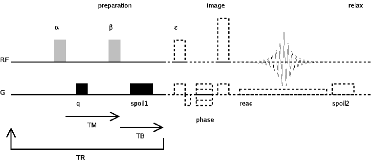
Figure 1: Pulse Sequence. All RF pulses shown as hard for simplicity are actually Sinc3. $\alpha$ and $\beta$ are the same phase.

2 Experimental Methods

In order to study the behavior of the steady state $M_{z}^{SS}(s)$ profile we have implemented a looped DDF preparation subsequence followed by a standard multiple-phase encode imaging sub-sequence. (Figure 1.) The $\alpha$ pulse excites the system, the gradient $G_{q}$ twists the transverse magnetization into a helix. $\beta$ rotates one component of the helix back into the longitudinal direction. For simplicity we have omitted the $180^{\circ}$ pulses used to create a spin echo during TM and/or TB sometimes present in DDF sequences. Also, we are only interested in $M_{z}(s)$ in this experiment, not the actual DDF-generated transverse signal. Looping the “preparation” sub-sequence thus creates the periodic $M_{z}(s)$ profile, spoils remaining transverse magnetization, and establishes $M_{z}^{SS}(s)$. The $\varepsilon$ pulse converts $M_{z}^{SS}(s)$ into transverse magnetization, allowing it to be imaged via the subsequent spin echo “image” sub-sequence. $M_{z}^{SS}(s)$ must be re-established by the “preparation” sub-sequence for each phase encode. After a suitably long full relaxation delay “relax,” the sequence is repeated to acquire the next k-space line. This is clearly a slow acquisition method because many $TR$ periods are required to reach steady state in the preparation before each k-space line is acquired. The sequence is intended as a tool to directly image the $M_{z}^{SS}(s)$ profile, verifying the $M_{z}^{SS}(s)$ that would occur in a steady state DDF sequence, not as a new imaging modality.

Figure 2: Theoretical values of $M_{z}(s)$. $M_{z}^{SS}(s)$is shown dashed $---$ as an envelope, $M_{z}^{SS,\,\beta}(s)$ is shown as a heavy line, $M_{z}^{SS,\,TB}(s)$ as a normal line. $\alpha=\beta=90^{\circ},\ TR=2s,\ TM=0ms,\ TB=100ms,\ \ T_{1}=1.4s$

3 Theory

The effect of the ”preparation” pulse sequence was first determined for a single iteration. The progress along the sequence is denoted by the the superscript.

Starting with fully relaxed equilibrium magnetization before the $\alpha$ pulse:

$$M_{z}^{Eq}(s)=M_{0}$$ (1)

after the $\alpha$ pulse, the mix delay $TM$ and the $\beta$ pulse we have:

$$M_{z}^{\beta}(s) =[A^{\beta}cos(q\,s)+B^{\beta}]\,M_{z}^{Eq}+C^{\beta}M_{0}$$ (2)

$$A^{\beta}=-sin(\alpha)\,e^{-\frac{TM}{T_{2}}}sin(\beta)$$

$$B^{\beta}=cos(\alpha)\,e^{-\frac{TM}{T_{1}}}cos(\beta)$$

$$C^{\beta}=(1-e^{-\frac{TM}{T_{1}}})\,cos(\beta)$$

The parameter $q=\frac{2\pi}{\lambda}$, where $\lambda$ is the helix pitch resulting from the applied gradient. Diffusion has been assumed to be negligible at the scale of $\lambda$. Note that $T_{2}$ is used in $A$ rather than $T_{2}^{*}$ when $G_{q}$ is larger than background inhomogeneity and susceptibility gradients.

After the build delay $TB$ we have:

$$M_{z}^{TB}(s)=[A^{TB}cos(q\,s)+B^{TB}]\,M_{z}^{Eq}(s)+C^{TB}M_{0}$$ (3)

$$A^{TB}=-sin(\alpha)\,e^{-\frac{TM}{T_{2}}}sin(\beta)\,e^{-\frac{TB}{T_{1}}}$$

$$B^{TB}=cos(\alpha)\,e^{-\frac{TB}{T_{1}}}cos(\beta)\,e^{-\frac{TB}{T_{1}}}$$

$$C^{TB}=[(1-e^{-\frac{TB}{T_{1}}})\,cos(\beta)-1]\,e^{-\frac{TB}{T_{1}}}+1$$

At the start of the next repetition, after a $TR$ period inclusive of $TM$ and $TB$ we have

$$M_{z}^{TR}(s)=[A^{TR}cos(q\,s)+B^{TR}]M_{z}^{Eq}(s)+C^{TR}\,M_{0}$$ (4)

$$A^{TR}=-sin(\alpha)\,e^{-\frac{TM}{T_{2}}}sin(\beta)\,e^{-\frac{TR-TM}{T_{1}}}$$

$$B^{TR}=cos(\alpha)\,cos(\beta)\,e^{-\frac{TR}{T_{1}}}$$

$$C^{TR}=[(1-e^{-\frac{TM}{T_{1}}})\,cos(\beta)-1]\,e^{-\frac{TR-TM}{T_{1}}}+1$$

If we apply the sequence $N$ times and re-arrange the terms we get the series:

$$M_{z}^{NxTR}(s)=M_{0}+M_{0\,}[A^{TR}cos(q\,s)+B^{TR}+C^{TR}-1]\sum\limits_{n=1}^{N}[A^{TR}cos(q\,s)+B^{TR}]^{n-1}$$ (5)

for the starting magnetization state after $N$ repetitions of the sequence.

Summing an infinite number of terms results in the expression for the steady state $M_{z}^{SS}(s)$ after a large number of TR periods:

$$M_{z}^{SS}(s)=M_{0}-M_{0\,}[\frac{A^{TR}cos(q\,s)+B^{TR}+C^{TR}-1}{A^{TR}cos(q\,s)+B^{TR}-1}]$$ (6)

One can then calculate the magnetization state after the $\beta$ pulse in the steady state:

$$M_{z}^{SS,\,\beta}(s)=[A^{\beta}cos(q\,s)+B^{\beta}]\,M_{z}^{SS}(s)+C^{\beta}M_{0}$$ (7)

and after $TB$:

$$M_{z}^{SS,\,TB}(s)=[A^{TB}cos(q\,s)+B^{TB}]\,M_{z}^{SS}(s)+C^{TB}M_{0}$$ (8)

We show graphs of Eq. [6], [7], and [8] in Figure 2 for $TR=2s$.

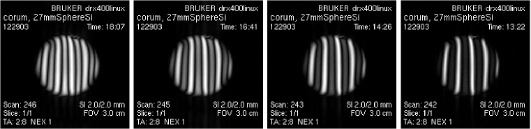
Figure 3: $M_{z}^{SS}(s)$ images, $TR=5s,\ 2s,\ 1s,\ 500ms$ from left to right. $TM=TB=\leavevmode\nobreak\ 7ms,\ relax=10s$.

4 Results

We now show in Figure 3 representative $M_{z}^{SS}(s)$ magnitude images obtained with the sequence described in section 2 for four different values of $TR=5s,\ 2s,\ 1s,\ 500ms$. Figure 4 shows several cross sections through row #128 of Figure 3. The object is an 18mm glass sphere filled with silicone oil. Data points are superimposed with the corresponding magnitude of the theoretical curve. The $T_{1}$ of the silicone oil (at 400MHz) was measured by spectroscopic inversion recovery to be 1.4s. A Bruker DRX400 Micro 2.5 system was used with a custom 27mm diameter 31P/1H birdcage coil. 10 $TR$ periods were used to establish steady state. A 10s “relax” delay was used between phase encodes to establish full relaxation. $G_{q}$ was 3ms and 2.5mT/mm, with $G_{spoil1}$ of 5ms and 100mT/mm. No attempt was made to account for $B_{1}$ inhomogeneity. A single scaling parameter was used for all theoretical curves. We achieved good agreement with the theoretical predictions. In the sequence as used $TM=TB=\leavevmode\nobreak\ 7ms$. A variety of other $G_{q}$ directions and strengths show similar agreement with theory. Better agreement in the fit between experiment and theory can be obtained with $\alpha=\beta=75^{\circ}$than with the nominal $90^{\circ}$. A $B_{1}$ map needs to be determined to see if this corresponds more closely to the actual experimental conditions.

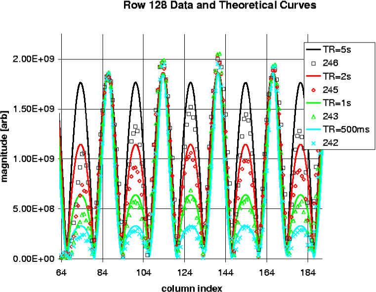
Figure 4: Row 128 data (points) and Fit (lines), $\alpha=\beta=90^{\circ},\ TR=2s,\ TM=TB=7ms,\ \ T_{1}=1.4s\ relax=10s$.

5 Conclusions

The expressions developed and verified above should be useful to those wishing to understand or utilize harmonics in the $M_{z}^{SS}(s)$ profile in DDF based sequences in the situation where the diffusion distance during $TR$ compared with $\lambda$ in negligible. This is especially true for those carrying out structural measurements which depend on a well defined correlation distance. The theory should also hold for spatially varying magnetization density $M_{0}=M_{0}(\vec{r})$, and longitudinal relaxation $T_{1}=T_{1}(\vec{r})$.

6 Acknowledgements

This work and preparation leading to it was carried out under the support of the Flinn Foundation, a State of Arizona Prop. 301 Imaging Fellowship, and NIH 5R24CA083148-05.

References

-
[1]
G. Deville, M. Bernier, J. Delrieux, NMR multiple echoes observed in solid
3He, Phys. Rev. B 19 (11) (1979) 5666–5688.
URL http://dx.doi.org/10.1103/PhysRevB.19.5666 - [2] R. Bowtell, R. M. Bowley, P. Glover, Multiple Spin Echoes in Liquids in a High Magnetic Field, J. Magn. Reson. 88 (3) (1990) 641–651.
-
[3]
I. Ardelean, S. Stapf, D. Demco, R. Kimmich, The Nonlinear Stimulated
Echo, J. Magn. Reson. 124 (2) (1997) 506–508.
URL http://dx.doi.org/10.1006/jmre.1996.1081 -
[4]
Q. He, W. Richter, S. Vathyam, W. Warren, Intermolecular multiple-quantum
coherences and cross correlations in solution nuclear magnetic resonance, The
Journal of Chemical Physics 98 (9) (1993) 6779–6800.
URL http://dx.doi.org/10.1063/1.464770 -
[5]
S. Ahn, N. Lisitza, W. Warren, Intermolecular Zero-Quantum Coherences of
Multi-component Spin Systems in Solution NMR, J. Magn. Reson.
133 (2).
URL http://dx.doi.org/10.1006/jmre.1998.1461 - [6] C. A. Corum, A. F. Gmitro, Effects of T2 relaxation and diffusion on longitudinal magnetization state and signal build for HOMOGENIZED cross peaks, in: ISMRM 12th Scientific Meeting, International Society of Magnetic Resonance in Medicine, 2004, poster 2323, cos(beta) should be (cos(beta)+1)/2 in abstract.
-
[7]
R. Bowtell, P. Robyr, Structural Investigations with the Dipolar
Demagnetizing Field in Solution NMR, Phys. Rev. Lett. 76 (26) (1996)
4971–4974.
URL http://dx.doi.org/10.1103/PhysRevLett.76.4971 -
[8]
W. Warren, S. Ahn, M. Mescher, M. Garwood, K. Ugurbil, W. Richter, R. Rizi,
J. Hopkins, J. Leigh, MR imaging contrast enhancement based on
intermolecular zero quantum coherences., Science 281 (5374) (1998) 247–51.
URL http://dx.doi.org/10.1126/science.281.5374.247 -
[9]
F. Alessandri, S. Capuani, B. Maraviglia, Multiple Spin Echoes in
heterogeneous systems: Physical origins of the observed dips, J. Magn.
Reson. 156 (1) (2002) 72–78.
URL http://dx.doi.org/10.1006/jmre.2002.2543