Chirped optical X-shaped pulses in material media${}^{\>({\dagger})}$

Michel Zamboni-Rached,

Department of Microwaves and Optics, School of Electrical Engineering (FEEC),

State University of Campinas, Campinas, SP, Brasil.

Hugo E. Hernández-Figueroa

Department of Microwaves and Optics, School of Electrical Engineering (FEEC),

State University of Campinas, Campinas, SP, Brasil.

Erasmo Recami

Facoltà di Ingegneria, Università statale di Bergamo, Dalmine (BG), Italy;

and  INFN—Sezione di Milano, Milan, Italy.

Abstract  –  In this paper we analyze the properties of chirped optical X-shaped pulses propagating in material media without boundaries. We show that such (”superluminal”) pulses may recover their transverse and longitudinal shape after some propagation distance, while the ordinary chirped gaussian-pulses can recover their longitudinal shape only (since gaussian pulses suffer a progressive spreading during their propagation). We therefore propose the use of chirped optical X-type pulses to overcome the problems of both dispersion and diffraction during the pulse propagation.

OCIS codes:  260.2030 ;  320.5550 ;  320.5540  ; 350.0350.

Keywords: Localized solutions to Maxwell equations; Optics; Superluminal waves; Bessel beams; Limited-diffraction pulses; Limited-dispersion pulses; X-shaped waves; Finite-energy waves; Electromagnetic wavelets; Electromagnetism.

1. – Introduction

Today, the theoretical and experimental existence of localized (nondiffracting) solutions to the wave equation in free space is a well established fact. The corresponding waves propagate for long distances resisting the diffraction effects, i.e., they maintain their shape during propagation; and the (Superluminal) X-shaped waves are examples of these solutions.

The theory of the localized waves (LWs) was initially developed for free space (vacuum)[1-4] and in some situations for waveguides (hollow or coaxial cables)[5]. Subsequently, the theory was extended in order to have undistorted wave propagation in material media without boundaries[6-13]. In this case the LWs are capable of overcoming both the difraction and dispersion problems for long distances. The extension of the LW theory to material media was obtained by making the axicon angle of the Bessel beams (BBs) vary with the frequency[6-13], in such a way that a (frequency) superposition of such BBs does compensate for the material dispersion.

In spite of such an idea to work well in theory[8] and in its possible experimental implementation[6,7], it is not a simply realizable one, and requires having recourse to holographic elements.

In this paper we propose a simpler way to obtain pulses capable of recovering their spatial shape, both transversally and longitudinally, after some propagation. It consists in using chirped optical X-type pulses, while keeping the axicon angle fixed. Let us recall that, by contrast, chirped gaussian pulses in unbounded material media may recover only their longitudinal width, since they undergo a progressive transverse spreading while propagating.

2. – Chirped optical X-shaped pulses in material media

Let us start with an axis-symmetric Bessel beam in a material medium with refractive index $n(\omega)$:

$$\psi(\rho,z,t)\;=\;J_{0}(k_{\rho}\rho)e^{i\beta z}e^{-i\omega t}\;,$$ (1)

where it must be obeyed the condition $k_{\rho}^{2}=n^{2}(\omega)\omega^{2}/c^{2}-\beta^{2}$, which connects amongs themselves the transverse and longitudinal wave numbers $k_{\rho}$ and $\beta$, and the angular frequency $\omega$. In addition, we impose that $k_{\rho}^{2}\geq 0$ and $\omega/\beta\geq 0$, to avoid a nonphysical behavior of the Bessel function $J_{0}(.)$ and to confine ourselves to forward propagation only.

Once the conditions above are satisfied, we have the liberty of writing the longitudinal wave number as $\beta=(n(\omega)\omega\cos\theta)/c$ and, therefore, $k_{\rho}=(n(\omega)\omega\sin\theta)/c$; where (as in the free space case) $\theta$ is the axicon angle of the Bessel beam.

Now we can obtain a X-shaped pulse by performing a frequency superposition of these BBs, with $\beta$ and $k_{\rho}$ given by the previous relations:

$$\Psi(\rho,z,t)\;=\;\int_{-\infty}^{\infty}\,S(\omega)\,J_{0}\left(\frac{n(\omega)\omega}{c}\sin\theta\,\rho\right)\,e^{i\beta(\omega)z}e^{-i\omega t}\,d\omega\;,$$ (2)

where $S(\omega)$ is the frequency spectrum, and the axicon angle is kept constant.

One can see that the phase velocity of each BB in our superposition (2) is different, and given by $V_{\rm phase}=c/(n(\omega)\cos\theta)$. So, the pulse given by Eq.(2) will suffer a dispersion during its propagation.

The method developed by Sõnajalg et al.[6,7] and explored by others[8-13], to overcome this problem, consisted in regarding the axicon angle $\theta$ as a function of the frequency, in order to obtain a linear relationship between $\beta$ and $\omega$.

Here, however, we want to work with a fixed axicon angle, and we have to find out another way for avoiding dispersion and diffraction along a certain propagation distance. To do that, we might choose a chirped Gaussian spectrum $S(\omega)$ in Eq.(2):

$$S(\omega)\;=\;\frac{T_{0}}{\sqrt{2\pi(1+iC)}}\,\,e^{\displaystyle{-q^{2}(\omega-\omega_{0})^{2}}}\;\;\;\;{\rm with}\;\;\;\;\;q^{2}\;=\;\frac{T_{0}^{2}}{2(1+iC)}\;,$$ (3)

where $\omega_{0}$ is the central frequency of the spectrum, $T_{0}$ is a constant related with the initial temporal width, and $C$ is the chirp parameter. Unfortunately, there is no analytical solution to Eq.(2) with $S(\omega)$ given by Eq.(3), so that some approximations are to be made.

Then, let us assume that the spectrum $S(\omega)$, in the surrounding of the carrier frequency $\omega_{0}$ , is enough narrow that $\Delta\omega/\omega_{0}<<1$, so to ensure that $\beta(\omega)$ can be approximated by the first three terms of its Taylor expansion in the vicinity of $\omega_{0}$: That is, $\beta(\omega)\approx\beta(\omega_{0})+\beta^{\prime}(\omega)|_{\omega_{0}}\,(\omega-\omega_{0})+(1/2)\beta^{\prime\prime}(\omega)|_{\omega_{0}}\,(\omega-\omega_{0})^{2}$; where, after using $\beta=n(\omega)\omega\cos\theta/c$, it results that

$$\frac{\partial\beta}{\partial\omega}\;=\;\frac{\cos\theta}{c}\left[n(\omega)+\omega\,\frac{\partial n}{\partial\omega}\right]\;\;;\;\;\frac{\partial^{2}\beta}{\partial\omega^{2}}\;=\;\frac{\cos\theta}{c}\left[2\frac{\partial n}{\partial\omega}+\omega\frac{\partial^{2}n}{\partial\omega^{2}}\right]\;.$$ (4)

As we know, $\beta^{\prime}(\omega)$ is related to the pulse group-velocity by the relation $Vg=1/\beta^{\prime}(\omega)$. Here we can see the difference between the group-velocity of the X-type pulse (with a fixed axicon angle) and that of a standard gaussian pulse. Such a difference is due to the factor $\cos\theta$ in Eq.(4). Because of it, the group-velocity of our X-type pulse is always greater than the gaussian one. In other words, $(V_{g})_{X}=(1/\cos\theta)(V_{g})_{gauss}$.

We also know that the second derivative of $\beta(\omega)$ is related to the group-velocity dispersion (GVD) $\beta_{2}$ by $\beta_{2}=\beta^{\prime\prime}(\omega)$.

The GVD is responsible for the temporal (longitudinal) spreading of the pulse. Here one can see that the GVD of the X-type pulse is always smaller than that of the standard Gaussian pulses, due the factor $\cos\theta$ in Eq.(4). Namely: $(\beta_{2})_{X}=\cos\theta(\beta_{2})_{\rm gauss}$.

On using the above results, we can write

$$\begin{array}[]{clcr}\Psi(\rho,z,t)\!\!&=\displaystyle{\frac{T_{0}\,\,e^{i\beta(\omega_{0})z}e^{-i\omega_{0}t}}{\sqrt{2\pi(1+iC)}}\,\int_{-\infty}^{\infty}\,J_{0}\left(\frac{n(\omega)\omega}{c}sin\theta\,\rho\right)\times}\\ \\ &\;\;\;\times\,\displaystyle{{\rm exp}\left\{i\frac{(\omega-\omega_{0})}{V_{g}}\left[z-V_{g}t\right]\right\}{\rm exp}\left\{(\omega-\omega_{0})^{2}\left[\frac{i\beta_{2}}{2}z-q^{2}\right]\right\}\,d\omega}\;.\end{array}$$ (5)

The integral in Eq.(5) cannot be solved analytically, but it is enough for us to obtain the pulse behavior. Let us analyze the pulse for $\rho=0$. In this case we obtain:

$$\Psi(\rho=0,z,t)\;=\;\displaystyle{e^{i\beta(\omega_{0})z}e^{-i\omega_{0}t}\,\frac{T_{0}}{\sqrt{T_{0}^{2}-i\beta_{2}(1+iC)z}}\,{\rm exp}\left[\frac{-(z-V_{g}t)^{2}(1+iC)}{2V_{g}^{2}[T_{0}^{2}-i\beta_{2}(1+iC)z]}\right]}\;.$$ (6)

From Eq.(6) we can immediately see that the initial temporal width of the pulse intensity is $T_{0}$ and that, after some propagation distance $z$, the time-width $T_{1}$ becomes

$$\frac{T_{1}}{T_{0}}\;=\;\left[\left(1+\frac{C\beta_{2}z}{T_{0}^{2}}\right)^{2}+\left(\frac{\beta_{2}z}{T_{0}^{2}}\right)^{2}\right]^{1/2}\;.$$ (7)

Relation (7) describes the pulse spreading-behavior. One can easily show that such a behavior depends on the sign (positive or negative) of the product $\beta_{2}C$, as is well known for the standard gaussian pulses[14].

In the case $\beta_{2}C>0$, the pulse will monotonically become broader and broader with the distance $z$. On the other hand, if $\beta_{2}C<0$ the pulse will suffer, in a first stage, a narrowing, and then it will spread during the rest of its propagation. So, there will be a certain propagation distance in correspondence to which the pulse will recover its initial temporal width ($T_{1}=T_{0}$). From relation (7), we can find this distance $Z_{T1=T_{0}}$ (considering $\beta_{2}C<0$) to be

$$Z_{T_{1}=T_{0}}\;=\;\frac{-2CT_{0}^{2}}{\beta_{2}(C^{2}+1)}\;.$$ (8)

One may notice that the maximum distance at which our chirped pulse, with given $T_{0}$ and $\beta_{2}$, may recover its initial temporal width can be easily evaluated from Eq.(8), and is results to be $L_{\rm disp}=T_{0}^{2}/\beta_{2}$. We’ll call such a maximum value $L_{\rm disp}$ the ”dispersion length”. It is the maximum distance the X-type pulse may travel while recovering its initial longitudinal shape. Obviously, if we want the pulse to reassume its longitudinal shape at some desired distance $z<L_{\rm disp}$, we have just to suitably choose the value of the chirp parameter.

The longitudinal shape-evolution described by Eq.(6) is shown in Fig.1, on adopting the chirp parameter $C=-1$ (and $\beta_{2}>0$).

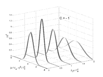
Figure 1:

We can notice that, initially, the pulse suffers a longitudinal narrowing with an increase of intensity till the position $z=T_{0}^{2}/2\beta_{2}$. After this point, the pulse starts to broaden decreasing its intensity and recovering its entire longitudinal shape (width and intensity) at the point $z=T_{0}^{2}/\beta_{2}$, as it was predicted above.

Let us emphasize that the property of recovering its own initial temporal (or longitudinal) width may be verified to exist also in the case of chirped standard gaussian pulses.[14]  However, the latter will suffer a progressive transverse spreading, which will not be reversible. The distance at which a gaussian pulse doubles its initial transverse width $w_{0}$ is $z_{\rm diff}=\sqrt{3}\pi w_{0}^{2}/\lambda_{0}$, where $\lambda_{0}$ is the carrier wavelength. Thus, we can see that optical gaussian pulses with great transverse localization will get spoiled in a few centimeters or even less.

Now we shall show that it is possible to recover also the transverse shape of the chirped X-type pulse intensity; actually, it is possible to recover its entire spatial shape after a distance $Z_{T_{1}=T_{0}}$.

To see this, let us go back to our integral solution (5), and perform the change of coordinates  $(z,t)\rightarrow(\Delta z,t_{c}=z_{c}/V_{g})$,  with

$$\left\{\begin{array}[]{l}z\;=\;z_{c}+\Delta z\\ \\ \displaystyle{t=t_{c}\equiv\frac{z_{c}}{V_{g}}}\end{array}\right.$$ (9)

where $z_{c}$ is the center of the pulse ($\Delta z$ is the distance from such a point), and $t_{c}$ is the time at which the pulse center is located at $z_{c}$. What we are going to do is to compare our integral solution (5), when $z_{c}=0$ (initial pulse), with that when $z_{c}=Z_{T_{1}=T_{0}}=-2CT_{0}^{2}/(\beta_{2}(C_{2}+1))$.

In this way, the solution (5) can be written, when $z_{c}=0$, as

$$\begin{array}[]{clcr}\Psi(\rho,z_{c}=0,\Delta z)\!\!&=\displaystyle{\frac{T_{0}\,\,e^{i\beta_{0}\Delta z}}{\sqrt{2\pi(1+iC)}}\,\int_{-\infty}^{\infty}\,J_{0}(k_{\rho}(\omega)\rho)\,{\rm exp}\left(\frac{-T_{0}^{2}}{2(1+C^{2})}(\omega-\omega_{0})^{2}\right)\times}\\ \\ &\;\;\;\displaystyle{\times\,{\rm exp}\left\{i\left[\frac{(\omega-\omega_{0})\Delta z}{V_{g}}+\frac{(\omega-\omega_{0})^{2}\beta_{2}\Delta z}{2}+\frac{(\omega-\omega_{0})^{2}T_{0}^{2}C}{2(1+C^{2})}\right]\right\}}\end{array}$$ (10)

where we have taken the value $q$ given by Eq.(3).

To verify that the pulse intensity takes on again its entire original form at $z_{c}=Z_{T_{1}=T_{0}}=-2\,CT_{0}^{2}/[\beta_{2}(C^{2}+1)]$, we can analyze our integral solution at that point, obtaining:

$$\begin{array}[]{clcr}\Psi(\rho,z_{c}=Z_{T_{1}=T_{0}},\Delta z)\!\!&=\displaystyle{\frac{T_{0}\,e^{i\beta_{0}(z_{c}-\Delta z^{\prime}-\frac{cz_{c}}{cos\theta\,n(\omega_{0})V_{g}})}}{\sqrt{2\pi(1+iC)}}\,\int_{-\infty}^{\infty}\,J_{0}(k_{\rho}(\omega)\rho)\,{\rm exp}\left(\frac{-T_{0}^{2}}{2(1+C^{2})}(\omega-\omega_{0})^{2}\right)\times}\\ \\ &\;\;\;\displaystyle{\times\,{\rm exp}\left\{-i\left[\frac{(\omega-\omega_{0})\Delta z^{\prime}}{V_{g}}+\frac{(\omega-\omega_{0})^{2}\beta_{2}\Delta z^{\prime}}{2}+\frac{(\omega-\omega_{0})^{2}T_{0}^{2}C}{2(1+C^{2})}\right]\right\}}\\ \end{array}$$ (11)

where we have put $\Delta z=-\Delta z^{\prime}$.  In this way, one immediately sees that

$$|\Psi(\rho,z_{c}=0,\Delta z)|^{2}=|\Psi(\rho,z_{c}=Z_{T_{1}=T_{0}},-\Delta z)|^{2}\;.$$ (12)

Therefore, from Eq.(12) it is clear that the chirped optical X-type pulse intensity reassumes its original three-dimensional form, with just a longitudinal inversion at the pulse center: The present method being, in this way, a simple and effective procedure for compensating the effects of diffraction and dispersion in an unbounded material medium; and a method simpler than the one of varying the axicon angle with the frequency.

Let us stress that we can choose the distance $z=Z_{T_{1}=T_{0}}\leq L_{\rm disp}$ at which the pulse will take on again its spatial shape by choosing a suitable value of the chirp parameter.

3. – Analytic description of the transverse pulse behavior during propagation

In the previous Section, we have shown that a chirped X-type pulse can recover its total three-dimensional shape after some propagation distance in material media, resisting, in this way, the effects of diffraction and dispersion.

We have also obtained an analytic description of the longitudinal pulse behavior (for $\rho=0$) during propagation, by means of Eq.(6). However, one does not get the same information about the transverse pulse behavior: We just know that it is recovered at $z=Z_{T_{1}=T_{0}}$).

Therefore, it would be interesting if we can get also the transverse pulse behavior in the plane of the pulse center $z=V_{g}t$. In that way, we’d get quantitative information about the evolution of the pulse-shape during its entire propagation.

To get this result, let us go back to Eq.(5) and rewrite the transverse wavenumber ($k_{\rho}=(n(\omega)\omega\sin\theta)/c$) in the more appropriate form

$$k_{\rho}\;=\;\displaystyle{\sqrt{\frac{n^{2}(\omega)\omega^{2}}{c^{2}}-\frac{n^{2}(\omega)\omega^{2}}{c^{2}}\cos\theta}}\;.$$ (13)

To analyze the transverse pulse behavior, it is enough to expand $n(\omega)\omega$ at the first order in the vicinity of the carrier frequency $\omega_{0}$

$$n(\omega)\omega\approx A\,u+B\;,$$ (14)

where $u\equiv(\omega-\omega_{0})$ and

$$A\;=\;\left(\omega_{0}\frac{\partial n}{\omega}|_{\omega_{0}}+n(\omega_{0})\right)\;=\;\frac{c}{V_{g}\,\cos\theta}\;,\;\;\;B\;=\;n(\omega_{0})\omega_{0}\;,$$ (15)

so that $k_{\rho}$ can be written as

$$k_{\rho}\approx\frac{\sin\theta}{c}\sqrt{A^{2}u^{2}+2ABu+B^{2}}$$ (16)

and the Bessel function of the integrand in Eq.(5) is given by

$$J_{0}(k_{\rho}(\omega)\rho)\;=\;J_{0}\left(\frac{\rho\sin\theta}{c}\sqrt{A^{2}u^{2}+2ABu+B^{2}}\right)\;.$$ (17)

Now, we use the identity

$$J_{0}(mR)\;=\;J_{0}(mx)J_{0}(my)+2\sum_{p=1}^{\infty}J_{p}(mx)J_{p}(my)\cos(p\phi)\;,$$ (18)

where $R=\sqrt{x^{2}+y^{2}-2xy\cos\phi}$.  In this way Eq.(17) can be written

$$\begin{array}[]{clcr}\displaystyle{J_{0}\left(\frac{\rho\sin\theta}{c}\sqrt{A^{2}u^{2}+2ABu+B^{2}}\right)}\!\!&=\displaystyle{J_{0}\left(\frac{\rho\sin\theta}{c}Au\right)J_{0}\left(\frac{\rho\sin\theta}{c}B\right)+}\\ \\ &\;\;\;\displaystyle{+2\sum_{p=1}^{\infty}J_{p}\left(\frac{\rho\sin\theta}{c}Au\right)J_{p}\left(\frac{\rho\sin\theta}{c}B\right)(-1)^{p}}\end{array}$$ (19)

On using this way of writing the Bessel function, and putting $z=z_{c}=V_{g}t$, we can integrate our solution (5) and, after some calculations and recourse to ref.[15], get

$$\begin{array}[]{l}\Psi(\rho,z=z_{c},t=z_{c}/V_{g})\;=\;\displaystyle{{\frac{T_{0}\,\,e^{i\beta(\omega_{0})z}e^{-i\omega_{0}t}}{\sqrt{2\pi(1+iC)}}}\ \displaystyle{{\frac{{\rm exp}\left(\displaystyle{{\frac{-\tan^{2}\theta\,\rho^{2}}{8\,V_{g}^{2}(-i\beta_{2}z_{c}/2\,+q^{2})}}}\right)}{\sqrt{-i\beta_{2}z_{c}/2\,+q^{2}}}}}}\\ \\ \\ \times\,\displaystyle{\left[\Gamma(1/2)J_{0}\left(\frac{n(\omega_{0})\,\omega_{0}\,\sin\theta\,\rho}{c}\right)I_{0}\left(\frac{\tan^{2}\theta\,\rho^{2}}{8\,V_{g}^{2}(-i\beta_{2}z_{c}/2\,+q^{2})}\right)\right.}\\ \\ \\ +\left.\displaystyle{2\sum_{p=1}^{\infty}\frac{2^{p}\Gamma(p+1/2)\Gamma(p+1)}{\Gamma(2p+1)}\,\,J_{2p}\left(\frac{n(\omega_{0})\,\omega_{0}\,\sin\theta\,\rho}{c}\right)I_{2p}\left(\frac{\tan^{2}\theta\,\rho^{2}}{8\,V_{g}^{2}(-i\beta_{2}z_{c}/2\,+q^{2})}\right)}\right]\\ \end{array}$$ (20)

where we used (15), and $I_{p}(.)$ is the modified Bessel function of the first kind of order $p$, quantity $\Gamma(.)$ being the gamma function and $q$ being given by Eq.(3).

Equation (LABEL:trans1) describes the transverse pulse behavior (in the plane $z=z_{c}=V_{g}t$) during its whole propagation. At a first sight, this solution could appear very complex, but the series in its right hand side gives a negligible contribution. This fact renders our solution (LABEL:trans1) of important practical interest.

Indeed, from this solution one can see that the transverse pulse width is governed either by the gaussian function

$${\rm exp}\displaystyle{\left(\frac{-\tan^{2}\theta\,\rho^{2}}{8\,V_{g}^{2}(-i\beta_{2}z_{c}/2\,+q^{2})}\right)}$$ (21)

or by the Bessel function

$$J_{0}\left(\frac{n(\omega_{0})\,\omega_{0}\,\sin\theta\,\rho}{c}\right)\;,$$ (22)

whose transverse width are given, respectively, by

$$\Delta\rho_{G}(z_{c})\;=\;\frac{2\,c\,\sqrt{(T_{0}^{2}+\beta_{2}Cz_{c})^{2}+\beta_{2}^{2}z_{c}^{2}}}{T_{0}\sin\theta\left(n(\omega_{0})+\omega_{0}\frac{\partial n}{\partial\omega}|_{\omega_{0}}\right)}$$ (23)

and by

$$\Delta\rho_{B}\;=\;\frac{2.4\,c}{n(\omega_{0})\omega_{0}\sin\theta}\;,$$ (24)

where we took advantage of the fact that $V_{g}=(c/\cos\theta)\partial(\omega n(\omega))/\partial\omega)|_{\omega_{0}}$, and approximated the first root of the Bessel function $J_{0}(.)$ by adopting the value $2.4$.

One can see from Eq.(23) that, when $\beta_{2}C<0$ (which correspond to the cases considered in this paper), the gaussian function (21) will suffer a progressive spreading till $z_{c}=-CT_{0}^{2}/\beta_{2}(1+C^{2})$; after this point, it will start to spread out with the distance $z_{c}$ in an irreversible way, recovering its initial value $\Delta\rho_{G}(z_{c}=0)$ at the point $z_{c}=Z_{T_{1}=T_{0}}=-2CT_{0}^{2}/\beta_{2}(1+C^{2})$, as we had forecast in Section 2.

On the other hand, from Eq.(24) we can see that the transverse width $\Delta\rho_{B}$ of the Bessel function (22) will be constant during propagation, since the it does not depend on $z_{c}$.

During its propagation, the pulse’s transverse width will be governed by that one, of the two functions (21) and (22), which possesses the smaller width.

For example, at the point $z_{c}=Z_{T_{1}=T_{0}}=-2CT_{0}^{2}/\beta_{2}(1+C^{2})$, we have that

$$\frac{\Delta\rho_{G}(z_{c}=Z_{T_{1}=T_{0}})}{\Delta\rho_{B}}\;=\;\frac{2n(\omega_{0})}{2.4\left(n(\omega_{0})+\omega_{0}\frac{\partial n}{\partial\omega}|_{\omega_{0}}\right)}\,\,T_{0}\omega_{0}$$ (25)

and we can see that the transverse pulse-width evolution will depend on the value of $T_{0}\omega_{0}$,  the initial temporal width $T_{0}$ being related with the pulse frequency bandwidth $\Delta\omega=(1+C^{2})^{1/2}/T_{0}$.

Here we can distinguish two different situations:

When

$$T_{0}\omega_{0}>\frac{2.4\left(n(\omega_{0})+\omega_{0}\frac{\partial n}{\partial\omega}|_{\omega_{0}}\right)}{2n\omega_{0}}$$

we have that $\Delta\rho_{B}<\Delta\rho_{G}(z_{c}=Z_{T_{1}=T_{0}})$, so that the transverse pulse width $\Delta\rho$  will be governed by the Bessel function (22), that is, $\Delta\rho=\Delta\rho_{B}=2.4\,c/(n(\omega_{0})\omega_{0}\sin\theta)$ (whose value will remain constant during the rest of the propagation).. The pulse intensity will suffer an intensity decrease due a longitudinal spreading that starts after $z_{c}=Z_{T_{1}=T_{0}}/2$.

When, by contrast,

$$T_{0}\omega_{0}<\frac{2.4\left(n(\omega_{0})+\omega_{0}\frac{\partial n}{\partial\omega}|_{\omega_{0}}\right)}{2n\omega_{0}}$$

we are dealing with ultrashort pulses, while supposing that $\beta_{2}$ is still enough to describe the material dispersion. In these situations, $\Delta\rho_{G}(z_{c}=Z_{T_{1}=T_{0}})<\Delta\rho_{B}$, so that the transverse pulse width $\Delta\rho$  will be governed by the gaussian function (21), that is, $\Delta\rho=\Delta\rho_{G}(z_{c})$, given by Eq.(23): And the pulse will suffer a progressive transverse spread during its propagation till the distance

$$z_{c}\;=\;\frac{\displaystyle{T_{0}^{2}|C|+\frac{T_{0}}{2n(\omega_{0})\omega_{0}}\sqrt{2.4^{2}(1+C^{2})\left(n(\omega_{0})+\omega_{0}\frac{\partial n}{\partial\omega}|_{\omega_{0}}\right)^{2}-\,4\,T_{0}^{2}\,n^{2}(\omega_{0})\,\omega_{0}^{2}}}}{|\beta_{2}|(1+C^{2})}\;,$$

where $\Delta\rho_{G}(z_{c})=\Delta\rho_{B}$.  From such a point onwards, the Bessel function (22) starts to rule the pulse transverse width, $\Delta\rho=\Delta\rho_{B}=2.4\,c/(n(\omega_{0})\omega_{0}\sin\theta)$, which will remain constant i the rest of the propagation.. Naturally, there will be a pulse intensity decrease due to the longitudinal spreading that takes place after $z_{c}=Z_{T_{1}=T_{0}}/2$.

It is interesting to notice that in both cases, the pulse, besides recovering its full three dimensional shape at $z_{c}=Z_{T_{1}=T_{0}}$, will reach, after some distance that depends on the considered case, a constant transverse width $\Delta\rho=2.4\,c/(n(\omega_{0})\omega_{0}\sin\theta)$, that is, the same width as that of a Bessel beam of frequency and axicon angle equal to the carrier frequency and axicon angle of the chirped X-type pulse.

Now, we can use Eq.(LABEL:trans1) to show the transverse behavior of a X-Type pulse propagating, e.g., in fused Silica ($SiO_{2}$) with the following characteristics: $T_{0}=0.4\;$ps, $\lambda_{0}=0.2\mu\;$m, and axicon angle $\theta=0.002\;$rad. For evaluating the quantity $\beta_{1}$, we need the refractive index function $n(\omega)$. Far from the medium resonances, it can be approximated by the well-known Sellmeier equation[14]

$$n^{2}(\omega)\;=\;\displaystyle{1\,+\,\sum_{j=1}^{N}\,\frac{B_{j}\,\omega_{j}^{2}}{\omega_{j}^{2}-\omega^{2}}}\;,$$ (26)

where $\omega_{j}$ are the resonance frequencies, $B_{j}$ the strength of the $j$th resonance, and $N$ the total number of the material resonances that appear in the frequency range of interest. For our purposes it is appropriate to choose $N=3$, which yields, for bulk fused Silica, the values[14] $B_{1}=0.6961663$;  $B_{2}=0.4079426$;  $B_{3}=0.8974794$;  $\lambda_{1}=0.0684043\;\mu\;$m;  $\lambda_{2}=0.1162414\;\mu\;$m;  and $\lambda_{3}=9.896161\;\mu\;$m.

Figure (2) shows the evolution of the transverse shape of such a pulse with chirp parameter $C=-1$   (so that $Z_{T_{1}=T0}=L_{\rm Disp}=T_{0}^{2}/\beta_{2}$). One can notice that the pulse maintains its transverse width $\Delta\rho=2.4\,c/(n(\omega_{0})\omega_{0}\sin\theta)=24.635\mu\;$m during its entire propagation due the fact that $T_{0}\omega_{0}>>1$; however, the same does not occur with the pulse intensity. Initially the pulse suffers an increase of intensity till the position $z_{c}=T_{0}^{2}/2\beta_{2}$; after this point, the intensity starts to decrease, and the pulse recovers its entire transverse shape at the point $z_{c}=T_{0}^{2}/\beta_{2}$, as it was expected by us. Here we have skipped the series on the right hand side of Eq.(LABEL:trans1), because, as we already said, it yields a negligible contribution.

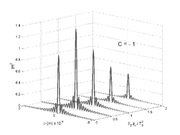
Figure 2:

4. – Advantages and limitations of using chirped X-type waves

The main advantage of the present method is its simplicity. A chirped optical X-type pulse with a constant axicon angle can be generated in a very simple way, by using an annular slit localized at the focus of a convergent lens, and illuminating that slit with a chirped optical gaussian pulse (where the chirp can be controlled directly in the laser modulation).

However, we should recall that we have taken into account the dispersion effects till their second order. When the pulse wavelength nearly coincides with the zero dispersion wavelength (i.e., $\beta_{2}\approx 0$), or when the pulse (depending on the material) is ultrashort, then it is necessary to include the third order dispersion term $\beta_{3}$, which in those cases will provide the dominant GVD effect. Consequently, the use of chirped optical X-type pulses might not furnish in those case the same results as shown above. A good option in such cases would be varying the axicon angle with the frequency.

Let us also recall that a Bessel beam, generated by finite apertures (as it must be, in any real situations), maintains its nondiffracting properties till a certain distance only (called its field depth), given by

$$L_{\rm diff}\;=\;\frac{R}{\tan\theta}\;,$$ (27)

where $R$ is the aperture radius and $\theta$ is the axicon angle. We call this distance $L_{\rm diff}$ to emphasize that it is the distance along which a X-type wave can resist the diffraction effects.

So, since our chirped X-type pulse is generated by a frequency superposition of BBs with the same axicon angle, our pulse will be able to take on again its shape at the position $z=Z_{T_{1}=T_{0}}\leq L_{\rm disp}$, if those BBs themselves are able to reach such a point resisting to the diffraction effects; in other words, if

$$Z_{T_{1}=T_{0}}\leq L_{\rm diff}\;\;\;\rightarrow\;\;\;\frac{-2CT_{0}^{2}}{\beta_{2}(C^{2}+1)}\leq\frac{R}{\tan\theta}$$ (28)

This fact leads us to conclude that the dispersion length $L_{\rm disp}$ and the diffraction length $L_{\rm diff}$ play important roles in the applications of chirped X-type pulses. Such roles are exploited (and summarized) in the following two cases:

First case:

When $L_{\rm disp}\leq L_{\rm diff}$:

In this case the dispersion plays the critical role in the pulse propagation, and we can ensure pulse fidelity till a maximum distance given by $z=L_{\rm disp}=T^{2}_{0}/\beta_{2}$. More specifically, we can choose a distance $z=Z_{T_{1}=T_{0}}\leq L_{\rm disp}$ at which the pulse will reassume its whole spatial shape by choosing the correct value of the chirp parameter.

Second case:

When $L_{\rm diff}\leq L_{\rm disp}$ :

In this case the diffraction plays the critical role in the pulse propagation. When this occurs, we can emit in the dispersive medium a chirped X-type pulse that takes on again its entire spatial shape after propagating till the maximum distance, given by $z=L_{\rm diff}$. To do this, we have to choose the correct value of the chirp parameter.

Let us suppose that we want the pulse intensity to reach the maximum distance $L_{\rm diff}$ with the same spatial shape as in the beginning. We should have, then:

$$\frac{-2CT_{0}^{2}}{\beta_{2}(C^{2}+1)}\;=\;\frac{R}{\tan\theta}\ .$$ (29)

Once $T_{0}$, $\beta_{2}$,  $R$ and  $\theta$ are known, we can use Eq.(29) to find the correct value of the chirp parameter.

5. – Comparison with the ordinary chirped gaussian pulses

It would be interesting if some comparison was made among the chirped X-type pulses and the ordinary chirped gaussian pulses.

In this comparison we will deal, with respect to the X-pulses, with the situation given by the first case in Section $4$; we will use the condition $L_{\rm diff}\geq 2\,L_{\rm disp}$.  Then, we can approximate a chirped X-type pulse, generated by finite apertures (finite energy), by having recourse to the equations previously obtained, at least till the distance $2L_{\rm disp}$.  On the contrary, one ought to use numerical simulations for obtaining the pulse behavior till that distance.

Now, on using the paraxial approximation, a chirped gaussian pulse of initial transverse width $w_{0}$, initial temporal width $T_{0}$, chirp parameter $C$ and carrier frequency $\omega_{0}$, and propagating in a material medium with refractive index $n(\omega)$, can be written as

$$\Psi_{\rm gaussian}(\rho,z,t)\;=\;\frac{\displaystyle{{\rm exp}\left(\displaystyle{\frac{-\rho^{2}}{w_{0}^{2}+2\,i\,z/k_{0}}}\right)\,{\rm exp}\left(\displaystyle{\frac{(z-V_{g}\,t)^{2}(1+i\,C)}{2\,V_{g}^{2}\,T_{0}^{2}(1-i\,(1+i\,C)\beta_{2}\,z/T_{0}^{2})}}\right)}}{\displaystyle{\left(1+\frac{2\,i\,z}{w_{0}^{2}\,k_{0}}\right)\,\sqrt{1-i\,(1+i\,C)\,\frac{\beta_{2}\,z}{T_{0}^{2}}}}}\;,$$ (30)

where $k_{0}=2\pi/\lambda_{0}=\omega_{0}/c$,  $V_{g}=1/\beta^{\prime}(\omega)|_{\omega_{0}}$,  $\beta_{2}=\beta^{\prime\prime}(\omega)|_{\omega_{0}}$  with  $\beta(\omega)=n(\omega)\omega/c$.

To perform the comparison, we will consider the following situation: Both pulses possess the same spot-size, the same carrier frequency and temporal width, the same chirp parameter, and propagate inside fused silica. The values of the group velocity, and the group velocity dispersion, of each pulse will be calculated by using the previous relations, the refractive index $n(\omega)$ being approximated by the Sellmeier equation (26).

Thus, we may consider a gaussian pulse with: $\lambda_{0}=0.2\mu\;$m,  $T_{0}=0.4\;$ps,  $C=-1$ and an initial transverse width (spot-size) $w_{0}=0.117\;$mm; Figure 3 shows the longitudinal and transverse behavior of this pulse during propagation.

We can see from Fig.3a that the chirped gaussian pulse may recover its longitudinal width, but with an intensity decrease, at the position given by $z=Z_{T_{1}=T_{0}}=L_{\rm disp}=T^{2}_{0}/\beta_{2}$ (because $C=-1$), which, in this case, is equal to $0.373\;$m. Its transverse width, on the other hand, suffers a progressive spreading and, in the considered case, doubles its value at the position $z=L_{\rm disp}=T^{2}_{0}/\beta_{2}=0.373\;$m, as one can see from Fig.3b.

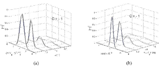
Figure 3:

Considering now in the same medium (fused silica) a chirped X-type pulse, with the same $\lambda_{0}$, $T_{0}$, $C$ and with an axicon angle $\theta=0.00084\;$rad, which correspond to an initial central spot with $\Delta\rho_{0}=0.117\;$mm (the same as for gaussian pulses), we get, during propagation, the longitudinal and transverse shapes represented by Fig.4.

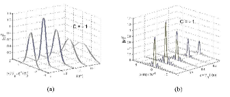
Figure 4:

As one can see from Figs.4a and 4b, the pulse recovers totally its longitudinal and transverse shape at the position $z=L_{\rm Disp}=T^{2}_{0}/\beta_{2}=0.373\;$m.

Again, we can notice that, during its entire propagation, the chirped X-type pulse maintains its transverse width $\Delta\rho=2.4\,c/(n(\omega_{0})\omega_{0}\sin\theta)=0.117\;$mm  (because $T_{0}\omega_{0}>>1$), decreasing however its intensity after $z=T_{0}^{2}/2\beta_{2}$ because of the progressive longitudinal broadening that occurs after that point. In the case of a finite-aperture generation, this behavior will be approximately maintained till $z=L_{\rm diff}=R/\tan\theta$.

Considering an aperture of radius $R=1\;$mm, the chirped X-type pulse considered above would have $L_{\rm diff}=1.186\;$m.

6. – Conclusions

In this paper we have proposed the use of chirped optical X-shaped pulses in dispersive media to overcome the problems of both diffraction and dispersion. We have shown that the dispersion and the diffraction length, $L_{\rm disp}$ and $L_{\rm diff}$, respectively, play essential roles on the recovering of the pulse-intensity shape.

Acknowledgements

The authors are very grateful to Amr Shaarawi for continuous discussions and collaboration. Useful discussions are moreover acknowledged with with J.M.Madureira, S.Zamboni-Rached, V.Abate, M.Brambilla, C.Cocca, R.Collina, C.Conti, G.C.Costa, G.Degli Antoni, G.Kurizki, G.Marchesini, D.Mugnai, M.Pernici, V.Petrillo, A.Ranfagni, G.Salesi, J.W.Swart, M.T.Vasconselos and M.Villa.

7. – Figure Captions

Fig.1 – Longitudinal-shape evolution of a chirped X-shaped pulse with $C=-1$. One can see that such a pulse recovers its full longitudinal shape at the position $z=L_{\rm disp}=T^{2}_{0}/\beta_{2}$.

Fig.2 – Transverse-shape evolution of a chirped X-type pulse with $C=-1$,  $T_{0}=0.4\;$ps,  $\lambda_{0}=0.2\mu\;$m, and axicon angle $\theta=0.002\;$rad, which correspond to an initial transverse width of $\Delta\rho=24.63\mu\;$m.  One can see that the pulse recovers its entire transverse shape at the distance $z=L_{\rm Disp}=T^{2}_{0}/\beta_{2}$: Which, in this case, is equal to $0.373\;$m.

Fig.3 –  (a): Longitudinal-shape evolution of a chirped gaussian pulse propagating in fused silica, with $\lambda_{0}=0.2\mu\;$m,  $T_{0}=0.4\;$ps,  $C=-1$ and initial transverse width (spot-size) $\Delta\rho_{0}=0.117\;$mm.   (b): Transverse-shape evolution for the same pulse.

Figs.4.  (a): Longitudinal-shape evolution of a chirped X-type pulse, propagating in fused silica with $\lambda_{0}=0.2\mu\;$m,  $T_{0}=0.4\;$ps,  $C=-1$ and axicon angle $\theta=0.00084\;$rad, which correspond to an initial transverse width of $\Delta\rho_{0}=0.117\;$mm.   (b): Transverse-shape evolution for the same pulse.

References:

[1] I.M.Besieris, A.M.Shaarawi and R.W.Ziolkowski, “A bi-directional traveling plane wave representation of exact solutions of the scalar wave equation”, J. Math. Phys., 30, 1254-1269 (1989).

[2] J.-y.Lu and J.F.Greenleaf, “Nondiffracting X-waves: Exact solutions to free-space scalar wave equation and their finite aperture realizations”, IEEE Trans. Ultrason. Ferroelectr. Freq. Control, 39, 19-31, (1992).

[3] For a review, see: E.Recami, M.Zamboni-Rached, K.Z.Nóbrega, C.A.Dartora, and H.E.Hernández-Figueroa, “On the localized superluminal solutions to the Maxwell equations”, IEEE Journal of Selected Topics in Quantum Electronics, 9, 59-73 (2003); and references therein.

[4] M.Zamboni-Rached, E.Recami, and H.E.Hernández-Figueroa, “New localized Superluminal solutions to the wave equations with finite total energies and arbitrary frequencies”, European Physical Journal D, 21, 217-228 (2002).

[5] See, e.g., M.Zamboni-Rached, E.Recami, and F.Fontana, “Localized Superluminal solutions to Maxwell equations propagating along a normal-sized waveguide”, Physical Review E, 64, article no.066603 (2001).

[6] H.Sõnajalg, P.Saari, “Suppression of temporal spread of ultrashort pulses in dispersive media by Bessel beam generators” Optics Letters, 21, 1162-1164 (1996).

[7] H.Sõnajalg, M.Ratsep, P.Saari, “Demonstration of the Bessel-X pulse propagating with strong lateral and longitudinal localization in a dispersive medium ” Optics Letters, 22, 310-312 (1997).

[8] M. Zamboni-Rached, K.Z. Nóbrega, H.E.Hernández-Figueroa, and E. Recami, “Localized Superluminal solutions to the wave equation in (vacuum or) dispersive media, for arbitrary frequencies and with adjustable bandwidth”, Optics Communications, 226, 15-23 (2003).

[9] C.Conti, and S.Trillo, “Paraxial envelope X waves”, Optics Letters, 28, 1090-1093 (2003).

[10] M.A.Porras, G. Valiulis and P. Di Trapani, “Unified description of Bessel X waves with cone dispersion and tilted pulses”, Physical Review E, 68, article no.016613 (2003).

[11] M.A.Porras, and I.Gonzalo, “Control of temporal characteristics of Bessel-X pulses in dispersive media”, Optics Communications, 217, 257-264 (2003).

[12] M.A.Porras, R.Borghi, and M.Santarsiero, “Suppression of dispersion broadening of light pulses with Bessel-Gauss beams”, Optics Communications, 206, 235-241 (2003).

[13] S. Longhi, “Spatial-temporal Gauss-Laguerre waves in dispersive media”, Physical Review E, 68, article no.066612 (2003).

[14] G.P.Agrawal, Nonlinear Fiber Optics (Academic Press; San Diego, CA, 1995).

[15] I.S.Gradshteyn, and I.M.Ryzhik, Integrals, Series and Products, 4th edition (Acad. Press; New York, 1965).