Dynamic effects in nonlinear magneto-optics of atoms and molecules

Abstract

A brief review is given of topics relating to dynamical processes arising in nonlinear interactions between light and resonant systems (atoms or molecules) in the presence of a magnetic field.

I Introduction

The study of resonant nonlinear magneto-optical effects (NMOE) is an active area of research with a rich history going back to the early work on optical pumping. These effects result from the resonant interaction of light with an atomic or molecular system in the presence of additional external electromagnetic fields (most commonly a uniform magnetic field, but we will also consider electric fields). A recent review by Budker et al.Budker et al. (2002a) deals primarily with the effects in atoms; the molecular case is detailed in a monograph by Auzinsh and Ferber.Auzinsh and Ferber (1995) In this paper, we focus on the dynamical aspects of such interactions, attempting to offer the reader a unified view on various diverse phenomena and techniques while avoiding excessive repetition of material already discussed in the previous reviews. Interest in the application of dynamic NMOE to experimental techniques has been increasing in recent years. The use of dynamic effects allows one to do things difficult with steady-state NMOE, for example, high-sensitivity Earth-field-range magnetometry. Dynamic effects can also allow information (such as the value of energy-level splittings) that would normally be obtained from high-resolution spectroscopy to be extracted from direct measurements of frequency, a more robust technique.

Nonlinear magneto-optical effects (specifically those related to coherence phenomenaBudker et al. (2002a)) are observed when a optically polarized medium undergoes quantum beats (Sec. II) under the influence of an external field, and so influences the polarization and/or intensity of a transmitted probe light beam. While this is inherently a dynamical process on the microscopic level, a macroscopic ensemble of particlesNot (a) reaches a steady state in about the polarization relaxation time if the external parameters are held constant. Thus, in order to observe quantum beat dynamics, these parameters must be varied at a rate significant compared to the polarization relaxation rate. One approach, discussed in Sec. III, is to produce polarization with a pulse of pump light, and then observe the effect of the subsequent quantum beat dynamics on the optical properties of the medium. Alternatively, the method of beat resonances (Sec. IV) can be used, in which an experimental parameter [the amplitude (Sec. IV.1), frequency (Sec. IV.2), or polarization (Sec. IV.3) of the light, the external field strength (Sec. IV.4), or the rate of polarization relaxation (Sec. IV.5)] is modulated, and the component of the signal at a harmonic of the modulation frequency is observed. Resonances are seen when the modulation frequency is a subharmonic of one of the quantum-beat frequencies present in the system.

II Quantum beats

Quantum beatsHaroche (1976); Dodd and Series (1978); Hack and Huber (1991); Aleksandrov et al. (1993); Auzinsh and Ferber (1995) is the general term for the time-evolution of a coherent superposition of nondegenerate energy eigenstates at a frequency determined by the energy splittings. In this paper, we are primarily concerned with the evolution of a polarized ensemble of particles with a given angular momentum that have their Zeeman components split by an external field. For linear Zeeman splitting—the lowest-order effect due to a uniform magnetic field—the evolution is Larmor precession, i.e., rotation of the polarization about the magnetic field direction. For nonlinear splittings, such as quadratic Stark shifts, the polarization evolution is more complex. The state of the ensemble is described by the density matrix, which evolves according to the Liouville equation. While this all that is necessary for a theoretical description of the system, physical insight can often be gained by decomposing the density matrix into polarization moments having the symmetries of the spherical harmonics. In quantum beats due to nonlinear energy splittings the relative magnitudes of the various polarization moments change with time, a process sometimes known as alignment-to-orientation conversion (see Refs. Budker et al., 2002a; Auzinsh and Ferber, 1995 and references therein). A pictorial illustration of the polarization state can be obtained by plotting its angular momentum probability distribution. The polarization moment decomposition and angular momentum probability distribution not only aid physical intuition, but they are themselves complete descriptions of the ensemble state, and can be used in some cases to simplify calculations. For a more detailed discussion, see Appendix A.

As an example, we consider the nonlinear Zeeman shifts that occur when atoms with hyperfine structure are subjected to a sufficiently large magnetic field. For states with total electron angular momentum $J=1/2$, such as in the alkali atoms, the shifted frequency $\omega_{m}$ of each Zeeman sublevel with spin projection $m$ along the magnetic field direction is given by the Breit-Rabi formulaAleksandrov et al. (1993)

$$\frac{\omega_{m}}{2\pi}=-\frac{\Delta}{2\left(2I+1\right)}-g_{I}\mu mB\pm\frac{\Delta}{2}\left(1+\frac{4m\xi}{2I+1}+\xi^{2}\right)^{1/2},$$ (1)

where $\xi=(g_{J}+g_{I})\mu B/\Delta$, $g_{J}$ and $g_{I}$ are the electronic and nuclear Landé factors, respectively, $B$ is the magnetic field strength, $\mu$ is the Bohr magneton, $\Delta$ is the hyperfine-structure interval, $I$ is the nuclear spin, and the $\pm$ sign refers to the upper and the lower hyperfine level, respectively. We set $\hbar=1$ throughout this paper.

Consider an atomic sample of cesium ($I=7/2$), initially in a stretched state ($m_{z}=F=4$) with respect to the $z$-axis. In the presence of an $\mathbf{\hat{x}}$-directed magnetic field, the energy eigenstates are the ${\left|Fm_{x}\right\rangle}$ eigenstates of the $F_{x}$ operator. The stretched state along $\mathbf{\hat{z}}$ is a superposition of these nondegenerate eigenstates, and so quantum beats are seen in the evolution of the system.

The time evolution of each eigenstate is given by $c_{m}\exp\left(-i\omega_{m}t\right){\left|Fm\right\rangle}$ where $c_{m}$ is the initial amplitude. For moderate field strengths such that the parameter $\xi$ is small, the shifts deviate only slightly from linearity. Thus, expanding Eq. (1) in powers of $\xi$, we see that over time scales comparable to the Larmor period, the evolution (to first order) is just Larmor precession with period $\tau_{1}\simeq 8(g_{J}\mu B)^{-1}$ (neglecting here $g_{I}$ compared to $g_{J}$). The evolution due to the second-order quadratic shifts is also periodic, but with a much longer period $\tau_{2}\simeq 32\Delta(g_{J}\mu B)^{-2}$. (For $B=0.5$ G, $\tau_{1}\simeq 6\ \mu$s and $\tau_{2}\simeq 0.3$ s.) One way to illustrate these quantum beats is to produce graphs of the spatial distribution of angular momentum at a given time. To do this, we plot three-dimensional closed surfaces for which the distance from the origin in a given direction is proportional to the probability of finding the maximum projection of angular momentum along that direction.Auzinsh (1997); Rochester and Budker (2001) This plot illustrates the symmetries of the polarization state, indicating which polarization moments are present. (For a discussion of the angular momentum probability distribution and the polarization moments, see Appendix A.) A collection of surfaces showing the time-evolution of the polarization over half of a period $\tau_{2}$ of the second-order evolution is shown in Fig. 1.

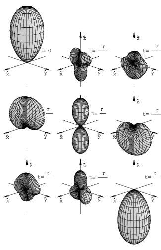
Figure 1: Quantum beats in Cs illustrated with surfaces representing the probability of finding the system in the state with maximal projection $m=F$ in a given direction.Auzinsh (1997); Rochester and Budker (2001) This sequence is “stroboscopic” in the sense that the surfaces correspond to times chosen to have the same phase of the fast Larmor precession around the direction of the magnetic field ($\mathbf{\hat{x}}$). From the symmetry of the plots one clearly sees that orientation present in the initial state collapses and revives in the process of the temporal evolution. Temporal variation of higher polarization moments give rise to higher-order-symmetry contributions to the probability surface (see also Fig. 3).

The first plot represents the initial stretched state—the surface is literally stretched in the $\mathbf{\hat{z}}$ direction. This state undergoes rapid precession around $\mathbf{\hat{x}}$ with period $\tau_{1}$. At the same time, the slower second-order evolution results in changes in the shape of the probability surface. By “stroboscopically” drawing successive surfaces each at the same phase of the fast Larmor precession (i.e., at integer multiples of $\tau_{1}$), the polarization can be seen to evolve into states with higher-order symmetry before becoming stretched along $-\mathbf{\hat{z}}$ at $t=\tau_{2}/2$. In particular, at $t=\tau_{2}/4$ the state is symmetric with respect to the $x$-$y$ plane, a characteristic of the even orders in the decomposition of the polarization state into irreducible tensor moments $\rho^{\kappa}$ (Appendix A). In general, for a multipole moment of rank $\kappa$ with polarization transverse to the quantization axis (such that only the components $\rho^{\kappa}_{q}$ with $q=\pm\kappa$ are nonzero) this moment has rotational symmetry of order $\kappa$ about that axisAuzinsh and Ferber (1991, 1995) (Fig. 2).

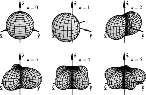
Figure 2: Angular momentum spatial distribution for states composed only of population ($\rho^{0}_{0}$) and the maximum possible values of the components $\rho^{\kappa}_{\pm\kappa}$ for a particular $\kappa$. $\kappa=0$: monopole moment (isotropic state with population only); $\kappa=1$: dipole moment (oriented state); $\kappa=2$: quadrupole moment (aligned state); $\kappa=3$: octupole moment; $\kappa=4$: hexadecapole moment; $\kappa=5$: triakontadipole moment.

In order to explore the decomposition into polarization moments further, it is useful to plot the normsRochester and Budker (2001) of the polarization moments as a function of time (Fig. 3).

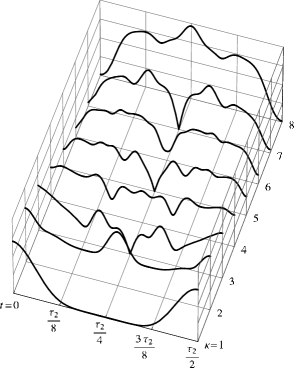
Figure 3: Temporal evolution of the norms of various polarization moments of ranks $\kappa$ of the $F=4$ ground state of Cs corresponding to the case of Figs. 1 and 4. The initial stretched state is dominated by the lowest-order moments; at $t=\tau_{2}/4$ the state is composed only of even-order moments.

The figure shows that initially the lowest-order moments predominate. At $t=\tau_{2}/4$ the odd-order moments are zero and the state is comprised of even-order moments only.

We can now connect these pictures of the atomic polarization state to an experimentally observable signal, e.g., the absorption of weak, circularly polarized light propagating along $\mathbf{\hat{z}}$. To find the absorption coefficient, assuming that the upper-state hyperfine structure is not resolved, we transform to the ${\left|J,m_{J}\right\rangle}{\left|I,m-m_{J}\right\rangle}$ basis with quantization axis along $\mathbf{\hat{z}}$ and sum over the transition rates for the Zeeman sublevels.

Figure 4: Collapse and revival beats arising in optically pumped Cs atoms due to nonlinearity of Zeeman shifts. (a) Time-dependent absorption of the probe light (see text) observed on a short time scale reveals an oscillation at the Larmor frequency. (b) Observation on a longer time scale reveals the characteristic collapse and revival (beating) behavior. Note period of essentially complete collapse of the oscillation pattern. (c) At even longer time scales, the beat pattern is modified due to third-order nonlinearity.

At short time scales [Fig. 4(a)] we see absorption modulated at the Larmor frequency, due to the precession of the atomic polarization about the $x$-axis. The absorption is minimal when the state is oriented along $\mathbf{\hat{z}}$, and maximal when it is oriented along $-\mathbf{\hat{z}}$. Looking at the envelope of this modulation at longer time scales, we see “collapse and revival” with period $\tau_{2}/2$ of the absorption oscillation amplitude [Fig. 4(b)]. The maxima of the envelope are associated with the stretched states shown in Fig. 1 and the minima with the states that are symmetric with respect to the $x$-$y$ plane. This can also be seen by comparison to Fig. 3; the envelope of the signal plotted in Fig. 4(b) is proportional to the norm of the $\kappa=1$ moment (orientation), and does not have any of the time-dependent behavior exhibited by the higher-order moments in Fig. 3. While it is true in general that weak probe light is not coupled to atomic polarization moments of rank greater than two,Dyakonov (1964) the fact that the absorption is insensitive to the $\kappa=2$ moment (alignment) is a consequence of our assumption that the upper-state hyperfine structure is unresolved. In Fig. 4(c) one can see the effect of the third-order terms in the expansion of (1), reducing the contrast of the envelope function.

Collapse and revival phenomena similar to the effect described here have been observed in nuclear precession.Majumder et al. (1990) In that work, spin precession of an $I=3/2$ system, ²⁰¹Hg, was studied and the slight deviations from linearity in the Zeeman shifts responsible for the collapse and revival beats were due to quadrupole-interaction shifts arising from the interaction of the atoms with the walls of a rectangular vapor cell. Collapse and revival phenomena in molecules with large angular momenta were considered in a tutorial paper. Auzinsh (1999)

III Transient dynamics

In order to observe macroscopic dynamics in the magneto-optical effects, some experimental parameter must be varied in time. Perhaps the most conceptually straightforward technique is to induce atomic or molecular polarization with a pulse of pump light and then observe the transient response. Quantum beats were originally observed in this way by detecting fluorescence.Aleksandrov (1964); Dodd et al. (1964) We are primarily concerned here with techniques involving probe light detection (a brief discussion of fluorescence experiments is given in Sec. VI.1). An early application of this method in conjunction with probe-light polarization spectroscopy was an experimentLange and Mlynek (1978) with ytterbium vapor. A 5 ns pulse of linearly polarized dye-laser light produced a coherently excited population in the ${\rm 6\,^{3}P_{1}}$ state, whose Zeeman sublevels were split by a magnetic field. The transmission of a subsequent linearly polarized probe-light pulse was observed through a crossed polarizer. Optical anisotropy in stimulated emission was observed as polarization rotation of the probe beam. The time dependence of the signal, due to the quantum-beat evolution (Larmor precession) of the excited-state polarization, was investigated indirectly by holding the probe-pulse delay time $\tau$ fixed, and sweeping the magnetic field. Oscillations corresponding to $\cos 2\Omega_{L}\tau$, where $\Omega_{L}$ is the Larmor frequency, were seen in the signal. The factor of two appears because linearly polarized light induces alignment (the $\kappa=2$ tensor moment), which has two-fold symmetry about any axis perpendicular to the alignment axis (Sec. II). Thus the quantum-beat frequency for this moment is $2\Omega_{L}$; in general, a rank $\kappa$ moment polarized as shown in Fig. 2 will have quantum-beat frequency $\kappa\Omega_{L}$ in a $\mathbf{\hat{z}}$-directed magnetic field.

Recently, nonlinear magneto-optical rotation with pulsed pump light was used to study the sensitivity limits of atomic magnetometry at very short time scales.Geremia et al. (2003, 2004) Observation of the time-dependence of optical rotation of a weak probe beam allows the measurement of the magnetic field to be corrected for the initial spin-projection uncertainty. For measurement times $T$ short enough that non-light-induced polarization relaxation processes can be neglected (in this case, $T\ll(\gamma\sqrt{N})^{-1}$, where $\gamma$ is the relaxation rate and $N$ is the number of polarized atoms), a “quantum nondemolition measurement”Scully and Zubairy (1997) can be performed by using far-detuned probe light. Over this time, a sub-shotnoise measurement with uncertainty scaling as $N^{-3/4}$ is then possible.Auzinsh et al. (2004) If squeezed lightScully and Zubairy (1997) is used, Heisenberg-limited scaling of $N^{-1}$ can be obtained, limited to an even shorter measurement time $T\ll(\gamma N)^{-1}$.

In the experiments discussed so far in this section, the measurement times were much shorter than the polarization relaxation time. When longer measurements are made, the amplitude of the quantum beats will be seen to decay during the measurement, due to mechanisms such as collisional relaxation and, for excited states, spontaneous emission.Not (b) An often important mechanism that has the effect of polarization relaxation is fly-through or transit relaxation. This results from polarized particles travelling out of the probe light beam while unpolarized particles enter the beam, resulting in a decrease in average polarization in the probe region. The effective rate of this relaxation $\gamma_{t}$ can be estimated from the average thermal velocity over the size of the relevant region. However, this relaxation is, in general, not described by an exponential decay with time constant $\gamma_{t}$, but in many cases can be substantially more complicated. For example, consider a situation in which, immediately after the pump pulse, particles are polarized in a spatial region that is larger than the probe region. This can occur even if the pump and probe beams have identical and overlapping profiles under conditions of nonlinear absorption: a strong Gaussian-profiled pump beam can perform efficient optical pumping even far away from the beam center. The weak probe, on the other hand, acts at the intensity range of linear absorption; it takes some time for particles in thermal motion to reach the beam center where they undergo the probe interaction. As a result, at the initial moments following the pump pulse, one does not observe significant effective relaxation. Only after a certain amount of time does fly-through relaxation set in. This effect was predicted and measured for relaxation of ground state K₂ molecules.Auzinsh et al. (1983) This nonexponential relaxation kinetics can be significant for quantitative analysis of quantum-beat signals.

In addition to the observation of transients, another way to study quantum beat dynamics is to use resonance techniques involving modulation of the external experimental conditions. Such techniques are discussed in the next section.

IV Beat resonances

IV.1 Amplitude resonances

In a pulsed experiment such as described in Sec. III, the quantum beats will tend to wash out as the pulse rate is increased relative to the polarization relaxation rate. Particles polarized during successive pulses will, in general, beat out of phase with each other, cancelling out the overall medium polarization. If the quantum-beat frequency is slower than the relaxation rate, each polarized particle will not be able to undergo an entire quantum-beat cycle before relaxing. Thus the quantum beats will not cancel completely, and there will be some residual steady-state polarization. This is the effect studied in the limiting case of steady-state NMOE experiments with cw pump light. If the quantum-beat frequency is faster than the relaxation rate, each particle will contribute to the average polarization over its entire quantum beat cycle, and the macroscopic polarization of the medium will be destroyed entirely. This is the reason that magnetometers based on steady-state NMOE lose sensitivity for Larmor frequencies greater than the relaxation rate. However, time-dependent macroscopic polarization can be regained—even for high quantum beat frequencies—if the pump light is pulsed or amplitude modulated at a subharmonic of the quantum-beat frequency.Not (c) Polarization is produced in phase with that of particles pumped on previous cycles. The light pulses contribute coherently to the medium polarization, and the ensemble beats in unison. This effect is known as synchronous optical pumping or “optically driven spin precession”.Bell and Bloom (1961a, b) This is a particular case of a general class of phenomena known as beat resonances,Aleksandrov (1963, 1964); Aleksandrov et al. (1993); Auzinsh and Ferber (1995) exhibited when a parameter of the pump light or external field is modulated, as discussed below. In NMOE experiments, such resonances are generally observed using lock-in detection of the transmission or polarization signal of the probe light, at a harmonic of the modulation frequency. However, in some cases, such as when total transmission (or fluorescence) is observed, the resonances can also be detected in the time-averaged signalAuzinsh (1990).

In 1961, Bell and BloomBell and Bloom (1961a) were the first to observe beat resonances, due to quantum beats in the ground states of Rb and Cs and in metastable He. The first ground-state quantum-beat resonance experiments in molecules were performed with Te₂Ferber et al. (1982) and were followed by experiments with K₂.Auzinsh et al. (1987, 1990) Synchronous optical pumping has been used over the years in many applications. To give just one example, this method was employed in sensitive searches Jacobs et al. (1995); Romalis et al. (2001a, b) for a possible permanent electric-dipole moment (whose existence is only possible due to a violation of both parity and time-reversal invariance) of ¹⁹⁹Hg.

IV.2 Frequency resonances

Frequency (rather than amplitude) modulation of the pump light can be used to produce an effect similar to that discussed in Sec. IV.1. Here, the optical pumping rate is modulated as a result of its frequency dependence. One example of this is nonlinear magneto-optical (Faraday) rotation with frequency-modulated light (FM NMOR). Budker et al. (2002b); Yashchuk et al. (2003); Malakyan et al. (2004) In this technique, linearly polarized light near-resonant with an atomic transition is directed parallel to the magnetic field. The frequency of the light is modulated, causing the rates of optical pumping and probing to acquire a periodic time dependence. As described in Sec. IV.1, a resonance occurs when the quantum-beat frequency $\kappa\Omega_{L}$ for a rank-$\kappa$ polarization moment equals the modulation frequency $\Omega_{m}$ (the lowest-order polarization moment here has $\kappa=2$). The atomic sample is pumped into a macroscopic rotating polarized state that causes a periodic modulation of the plane of light polarization at the output of the medium. The amplitude of time-dependent optical rotation at various harmonics of $\Omega_{m}$ can be measured with a phase-sensitive lock-in detector (Fig. 5).

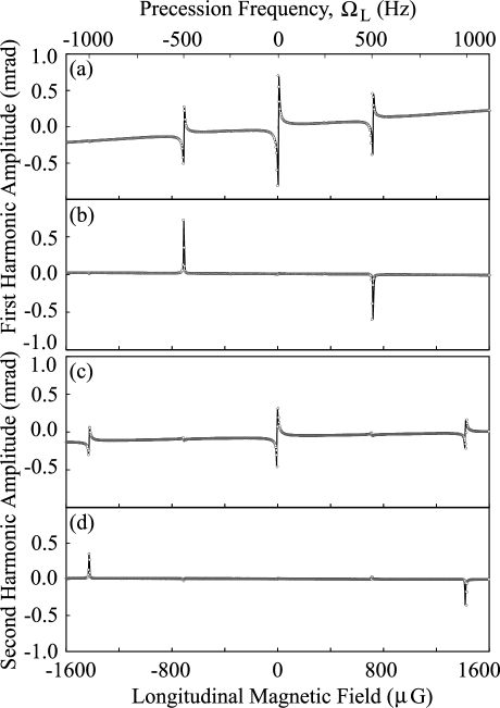
Figure 5: Signals detected at the first harmonic (a,b) and second harmonic (c,d) of $\Omega_{m}$ as a function of longitudinal magnetic field. This experiment employed buffer-gas-free, paraffin-coated vapor cells containing isotopically enriched ⁸⁷Rb. The laser was tuned near the $D1$ line, laser power was 15 $\mu$W, beam diameter $\sim$2 mm, $\Omega_{m}=2\pi\times 1$ kHz, and the modulation amplitude $\Delta\omega_{m}=2\pi\times 220$ MHz. Traces (a,c) and (b,d) correspond to the in-phase and the quadrature outputs of the signals from the lock-in detector, respectively. The zero-field resonances observed in traces (a,c) are similar in nature to the resonances observed in static NMOE studies (see text). The quadrature components arise because of a phase difference between the “probe” modulation and the modulation of the optical properties of the atomic medium. (Aligned atoms produce maximum optical rotation when the alignment axis is at an angle of $\pi/4$ to the light polarization direction.) Figure from Ref. Budker et al., 2002b.

Additional resonances can be observed when the quantum-beat frequency is equal to higher harmonics of the modulation frequency (equivalently, $\Omega_{m}$ is equal to subharmonics of the beat frequency $2\Omega_{L}/n$, where $n$ is the harmonic order).

As discussed in Sec. IV.1, in a steady-state nonlinear magneto-optical rotation experiment, the equilibrium polarization of the ensemble depends on the balance of Larmor precession with various mechanisms causing the polarization to relax (e.g., spin-exchange collisions or wall collisions). When the Larmor frequency is much less than the relaxation rate, the magnitude of the optical rotation increases linearly with the Larmor frequency. When the Larmor frequency increases, polarization is washed out and optical rotation falls off. Such zero-field resonances are also observed in the magnetic field dependence of the in-phase FM NMOR signals (Fig. 5). For the zero-field resonances, $\Omega_{m}$ is much faster than both $\Omega_{L}$ and the optical pumping rate for the cell, so the frequency modulation does not significantly affect the pumping process. On the other hand, as the laser frequency is scanned through resonance, there arises a time-dependent optical rotation, so the signal contains various harmonics of $\Omega_{m}$.

The FM NMOR technique is useful for increasing the dynamic range of NMOR-based magnetometers (Sec. V.2). The beat resonances have width comparable to that of the zero-field resonance (since the dominant relaxation mechanisms are the same), but in principle can be centered at any desired magnetic field.

IV.3 Polarization resonances

In addition to beat resonances obtained by modulation of the light amplitude and frequency, resonances due to modulation of light polarization have also been studied (for a review of earlier work, see Ref. Aleksandrov, 1972). These polarization resonances (also called phase resonances) are much like the other light modulation effects discussed above. Polarization modulation can be thought of as out-of-phase amplitude modulation of the light polarization components, providing a conceptual link to amplitude resonances (Sec. IV.1).

For Zeeman beats, the light polarization, when rotated at the Larmor frequency, is always parallel to the alignment of the ensemble. In this case, optical pumping contributes continuously and coherently to a rotating aligned polarization state of the ensemble. This effect was studied in an experimentBudker et al. (1999) with Rb. A $\lambda/2$ plate on a motor-driven rotating optical mount was used to continuously rotate the light polarization direction at a fixed frequency; transmission was observed with lock-in detection at this frequency while the longitudinal magnetic field strength was swept (Fig. 6).

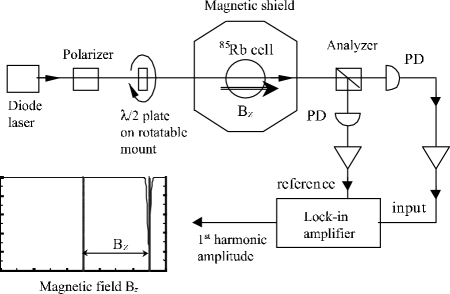
Figure 6: Experimental arrangement for the polarization resonance study.

The “dark resonance”, a drop in transmission, is normally centered at zero field when light polarization is fixed [Fig. 7(b)]. This resonance was shifted by the polarization rotation frequency [Fig. 7(c)].

Figure 7: Faraday rotation angle (a) and transmission (b) dependences on magnetic field recorded with stationary linear polarization of light. Trace (c) shows light transmission as a function of magnetic field when the linear polarization is rotated at $\Omega_{m}=2\pi\times 14$ Hz. Coil current of one $\mu$A corresponds to a magnetic field of approximately one $\mu$G.

Polarization resonances occurring in molecules have been analyzed theoretically.Auzinsh (1990) In that work, the time-averaged fluorescence intensity was considered as the method of detection.

IV.4 Parametric resonances

As mentioned in Sec. IV.1, one way to obtain beat resonances is to modulate the external field (e.g., the magnetic field), and consequently the Larmor precession frequency. This method has been used for sensitive atomic magnetometry,Dupont-Roc (1970) and is presently employed as a useful general nonlinear-spectroscopic techniqueFailache et al. (2003) known as parametric resonance.

In a typical setup (Fig. 8), linearly polarized resonant laser light traverses the medium, to which a magnetic field parallel to the light-propagation direction is applied.

Figure 8: A schematic of an experimental arrangement for parametric resonance spectroscopy with magnetic-field modulation.

The magnetic field has two components—a nearly dc component (that can be slowly scanned) and an ac component with frequency much faster than the ground-state polarization-relaxation rate. Transmitted light intensity is monitored with a photodetector, the signal from which is analyzed with a lock-in amplifier referenced to the ac modulation of the magnetic field.

As in FM NMOR (Sec. IV.2, Fig. 5), there are two types of resonances that are seen when the dc magnetic field is scanned: the zero-field resonance (independent of the ac-modulation frequency) that only appears in the in-phase component of the signal, and the frequency-dependent resonances in both the in-phase and quadrature components. The former arise because for resonant light the transmission is a quadratic function of the magnetic field, while the latter are due to an effective modulation of the rate of polarization production. As the ac field adds to or subtracts from the static field, it leads to acceleration or deceleration of the Larmor precession, respectively. Since, as discussed in Sec. IV.1, Larmor precession acts to average out the macroscopic polarization induced by cw pump light, more overall polarization is generated when the Larmor precession rate is the slowest. As a result, the rate of polarization production is modulated at the ac frequency, and so, as for amplitude or frequency resonances, a beat resonance occurs when the modulation frequency is a subharmonic of the quantum beat frequency.

IV.5 Parametric relaxation resonances

Beat resonances can also arise when the parameter that is modulated is the relaxation rate of the atomic polarization. Once again, resonances occur when the frequency of the modulation coincides with the spin-precession frequency or its subharmonic. This effect was predicted theoretically Okunevich (1974a); Novikov (1974) and observed experimentally Okunevich (1974b) in metastable helium, where relaxation rate was modulated by modulating the discharge current in a helium cell. Note that since relaxation is independent of the direction of the atomic spins (isotropic relaxation), this method, in contrast to the ones discussed above, cannot produce large overall polarizations of the sample when the Larmor precession rate significantly exceeds the relaxation rate (see Sec. IV.1).

We also briefly mention here another related dynamic magneto-optical effect: a sudden change in the relaxation or optical pumping rate for a driven spin system can cause transient spin-nutations Aleksandrov et al. (1987) while the system relaxes towards its new equilibrium state.

IV.6 Relation to coherent population trapping

An equivalent description of the beat resonance phenomena can be given in terms of coherent population trapping (CPT), an effect that is also closely related to $\Lambda$-resonances and mode crossing (see Ref. Arimondo, 1996 for a review). Indeed, harmonic modulation of the light intensity leads to the appearance of two sidebands at frequencies shifted from the unperturbed light frequency $\omega_{0}$ by the value of the modulation frequency: $\omega_{1,2}=\omega_{0}\pm\Omega_{m}$. With modulation depth less than 100%, the spectral component with frequency $\omega_{0}$ also survives [Fig. 9(a)].

Figure 9: (a) Light frequency spectrum for light-intensity modulation with 50% depth. (b) A CPT resonance at double modulation frequency in the case of a $F=1\rightarrow F^{\prime}=0$ transition. The lower-state Zeeman sublevels are split in a magnetic field applied along the quantization axis. (c) The CPT resonances in the case of frequency modulation with a large modulation index.

A CPT resonance occurs when the frequency difference between a pair of spectral components of the modulated light coincides with the frequency splitting of the lower-state Zeeman sublevels, so that light is resonant with a pair of transitions.Arimondo (1996) For a $F=1\rightarrow F^{\prime}=0$ transition [Fig. 9(b)], a CPT resonance leads to transfer of population from the “bright” state to the “dark” states that are uncoupled to the light, and light transmission increases. For harmonic modulation of the light intensity, there are two spectral difference frequencies ($\Omega_{m},2\Omega_{m}$), each resulting in an observed resonanceBell and Bloom (1961a) when the difference becomes equal to $2\Omega_{L}$, the splitting between the $M=1$ and $M=-1$ energy levels.

CPT resonances can also occur when the light is frequency modulated. In this case, the light spectrum consists of an infinite number of sidebands with amplitudes of the $n$th sideband given by a Bessel function $J_{n}(m)$ corresponding to the modulation index $m=\Delta\omega_{m}/\Omega_{m}$, where $\Delta\omega_{m}$ is the modulation depth. For example, an experimentAndreeva et al. (2003) with cesium atoms studied the application of the CPT effect with frequency-modulated light to atomic magnetometry. The value of the modulation index was $m\simeq 1.5$, so only a few sidebands were prominent. Both vacuum and buffer-gas cells were used, and the minimum observed width of the CPT resonance was 1.4 kHz in the latter case. The width of the resonance sets the lower bound on the magnetic fields (and, correspondingly, the resonance frequency) for which the resonances can be resolved.

The situation changes somewhat if the modulation index becomes large. For example, in the nonlinear magneto-optical rotation with frequency-modulated light experiments described in Sec. IV.2 the modulation depth is $\Delta\omega_{m}\simeq 30$ MHz and the modulation rate is $\Omega_{m}\simeq 100$–1000 Hz.Budker et al. (2002b); Yashchuk et al. (2003); Malakyan et al. (2004) Thus $m\simeq 10^{5}$ and the pairs of $\Delta M=2$ sublevels are coupled by a very large number of frequency-sideband pairs with comparable amplitude [Fig. 9(c)]. For this reason, the description in terms of the CPT-resonances is less intuitive here than the synchronous-pumping picture presented in Sec. IV.2.

V Applications

V.1 High-order polarization moments

The use of Zeeman beat resonances allows one to directly create and detect higher-order polarization moments. Because a polarization moment with rank $\kappa$ has symmetry of order $\kappa$ about some axis (Sec. II), a resonance in both pumping and probing due to interaction with this moment occur when the light-particle interaction is modulated at the frequency $\Omega_{m}=\kappa\Omega_{L}$. A dipole transition can connect polarization moments with ranks differing by at most two. Consequently, multiple photon interactions are required to generate high-rank polarization moments. For example, two interactions are required to produce a rank $\kappa=4$ hexadecapole moment from an initially unpolarized ($\kappa=0$) state. There must be an equal number of photon interactions in order to detect a signal due to the high-order multipole moment, which will be modulated at $\kappa\Omega_{L}$. Thus the amplitude of the signal due to the hexadecapole resonance scales as the fourth power of the light intensity, as experimentally observedYashchuk et al. (2003) in FM NMOR (Sec. IV.2).

Figure 10 shows the magnetic-field dependence of FM NMOR signals from a paraffin-coated cell containing ⁸⁷Rb in which the atoms are pumped and probed with a single light beam tuned to the $D1$ transition.

Figure 10: An example of the magnetic-field dependence of the FM NMOR signals showing quadrupole resonances at $B=\pm 143.0$ $\mu$G, and the hexadecapole resonances at $\pm 71.5$ $\mu$G. Laser modulation frequency is 200 Hz, modulation amplitude is 40 MHz peak-to-peak; the central frequency is tuned to the low-frequency slope of the $F=2\rightarrow F^{\prime}=1$ absorption line. Plots (a,b) show the in-phase component of the signal at two different light powers; plot (c) shows the quadrature component. Note the increase in the relative size of the hexadecapole signals at the higher power. The insets show zooms on hexadecapole resonances. Figure from Ref. Yashchuk et al., 2003.

At relatively low light power [Fig. 10(a)], there are three prominent resonances: one at $B=0$, and two corresponding to $2\Omega_{L}=\Omega_{m}$ (see Sec. IV.2, Fig. 5). Much smaller signals, whose relative amplitudes rapidly grow with light power, are seen at $4\Omega_{L}=\Omega_{m}$, the expected positions of the hexadecapole resonances.

Various experimental signatures of high-rank polarization moments were previously detected with other techniques, Suter et al. (1993); Suter and Marty (1994); Xu et al. (1997a, b); Matsko et al. (2003) but by taking advantage of the unique periodicity of the dynamic optical signals using beat resonances, such high-rank moments can be directly created, controlled, and studied. Because of the enhanced optical nonlinearities and different relaxation properties, higher-order polarization moments are of particular interest for application in many areas of quantum and nonlinear optics. In addition, when performing high-field magnetometry in alkali atoms (Sec. V.2), the use of the highest-order polarization moment supported by a given state may be advantageous, because its evolution is free of complications due to nonlinear dependence of the Zeeman shifts on the magnetic field.Yashchuk et al. (2003)

V.2 Magnetometry

The steady-state NMOE are a valuable tool for magnetometry; it has been shownBudker et al. (2000) that the sensitivity of a magnetometer based on nonlinear Faraday rotation can reach $\sim$$10^{-11}\,{\rm G\,Hz^{-1/2}}$. Dynamic techniques can provide useful extensions to the steady-state methods—in particular, they can be used to increase the magnetometer’s dynamic range by translating the narrow zero-field resonances to higher magnetic fields. As discussed in Sec. IV.2, steady-state NMOE lose sensitivity to magnetic fields when the Larmor frequency is greater than the polarization relaxation rate. If beat resonances are used for magnetic field detection, however, the dependence of the resonance condition on the modulation frequency can be used to tune the response of the system to a desired magnetic field range.

While the earliest examples of beat resonance magnetometry used amplitudeBell and Bloom (1961a) or parametricCohen-Tannoudji et al. (1969); Dupont-Roc (1970) resonances, in recent years the use of light-frequency modulation has become more common.Cheron et al. (1995, 1996); Gilles et al. (2001); Budker et al. (2002b) This is a result of the development and broad use of single-mode diode-laser systems. For such lasers, frequency modulation via the diode current and/or the cavity length controlled with a piezoelectric transducer voltage can be simpler and more robust than either light amplitude modulation or modulation of the applied magnetic field. However, such frequency modulation is usually accompanied with inevitable intensity modulation of up to $\sim$15%.Gilles et al. (2001) The deleterious effects of parasitic modulation and of laser-intensity noise can be avoided by detecting optical rotationBudker et al. (2002b) rather than transmission.

The use of beat resonances to selectively address high-rank polarization moments (Sec. V.1) can also be an advantage in magnetometry. Detection of such polarization moments may result in increased statistical sensitivity by allowing the use of higher light power without significant increase in the polarization relaxation rate due to power broadening.Yashchuk et al. (2003)

One possible application of beat resonance magnetometers is to low-field and remote-detection nuclear magnetic resonance and magnetic-resonance imaging. Both parametric resonanceCohen-Tannoudji et al. (1969) and FM NMOR magnetometersYashchuk et al. (2004) have been used to measure the nuclear magnetization of a gaseous sample placed near a “probe” Rb-vapor cell. In the latter work, the fields—due to xenon that was polarized by spin-exchange collisions with laser-polarized Rb–were in the nanogauss range.

VI Related topics

VI.1 Fluorescence detection

Another standard technique for the observation of quantum beats is the detection, not of polarization or transmission of a probe beam, but of spontaneous emission from an excited state. Quantum beats in fluorescence induced by weak probe light after pulsed excitation were experimentally observed for the first time in an experimentAuzinsh et al. (1985, 1986) measuring the magnetic moment of the ($v^{\prime\prime}=1,J^{\prime\prime}=73$) rovibronic level of the ground electronic state $X^{1}\Sigma_{g}^{+}$ of K₂ molecules. Many molecules have ${}^{1}\Sigma$ ground states. The magnetic moment of these states is nominally zero—nonzero corrections appear only because of mixing with other states due to perturbation by molecular rotation.Lefebvre-Brion and Field (2004) This makes calculations of magnetic moments in ${}^{1}\Sigma$ states rather complicated and experimental measurements of these moments become important.

As noted in Sec. V.1, a single-photon dipole interaction couples polarization moments with a difference in rank $\Delta\kappa\leq 2$. Since the absorption and re-emission of probe light is a two-photon process, moments up to rank four can be observed in fluorescence induced by single-photon excitation. Indeed, excited-state alignment will be directly connected by a dipole transition to all existing ground-state moments from population ($\kappa=0$) to the hexadecapole moment ($\kappa=4$). This technique was used in the study of the K₂ ground state for the first observationAuzinsh and Ferber (1984); Auzinsh et al. (1987, 1990) of a beat resonance due to the hexadecapole moment (Fig. 11).

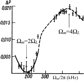
Figure 11: Ground-state beat-resonance signal measured as a change of the degree of polarization of laser induced fluorescence as a function of modulation frequency $\Omega_{m}$ of excitation light. The experiment was done with K₂ molecules. Two resonances, at twice (alignment) and four times (hexadecapole moment) the Larmor frequency $\Omega_{L}$, were observed. Figure from Ref. Auzinsh and Ferber, 1984.

Relaxation dynamicsAuzinsh et al. (1983) and Zeeman beatsAuzinsh et al. (1986) of multipole moments up to hexadecapole in K₂ molecules were also observed using pulsed pump light and fluorescence detection.

So far, we have discussed quantum beats arising due to the temporal evolution of the ground state. Obviously, one can also detect quantum beats in excited-state dynamics by observing fluorescence after pulsed excitation. This technique was used for the first observations of quantum beats in atoms, in experiments with the $6^{3}P_{2}$ stateAleksandrov (1964) of Hg and the $5^{3}P_{1}$ stateDodd et al. (1964) of Cd. In diatomic molecules, quantum beats from an excited state were first observedWallenstein et al. (1974) with iodine dimers in the $B^{3}\Pi_{0_{u}^{+}}$ state.

Quantum-beat studies measuring fluorescence from metastable states have been done as part of efforts to improve the present-day limitRegan et al. (2002) on the parity- and time-reversal-invariance-violating permanent electric-dipole moment (EDM) of the electron.DeMille et al. (2001) Close-lying states of opposite parity that can be mixed by a static electric field are advantageous for EDM measurements. The $J=1$ level of the first electronic excited state of lead oxide (PbO), $a(1)\ \left[{}^{3}\Sigma^{+}\right]$ is split into two opposite-parity states (the $\Omega$-doubletHerzberg (1989)) separated by only about 11 MHz. A recent experimentKawall et al. (2004) studied quantum beats in fluorescence from molecules excited by a dye-laser pulse to the $J=1$ states of $a(1)(v^{\prime}=5)$. For an EDM measurement it is necessary to measure small shifts with great accuracy; a sensitivity of about $50\$Hz/$\sqrt{\rm{Hz}}$ was demonstrated,Kawall et al. (2004) consistent with shot noise in the experiment. Precision measurements of the Landé factors of the two components of the $\Omega$-doublet were also made, laying the groundwork for a future EDM measurement. Quantum-beat measurements have also been done in atoms to evaluate metastable states for use in an EDM measurement: precision tensor polarizability measurements were done with Stark-induced quantum beats in Sm.Rochester et al. (1999) Also, a pair of long-lived opposite-parity states in Dy that are separated by only 3 MHz were studied.Budker et al. (1994) These states, components of which can be brought to crossing by applying a weak static magnetic field, were used in a quantum-beat technique to search for effects due to parity violation.Nguyen et al. (1997)

VI.2 Polarization-noise spectroscopy

An unpolarized medium clearly can not produce a net quantum beat signal. However, even in an unpolarized sample the randomizing processes that relax polarization at a rate $\gamma$ cause the medium polarization to fluctuate around its average value of zero. Since polarization created at a given time persists for an average time $1/\gamma$, the polarization noise spectrum contains only components at frequencies less than $\sim$$\gamma$ in the absence of an external field. When a magnetic field is applied, the polarization produced at a given time undergoes quantum beats, and so the detected signal in probe light propagating along the magnetic field direction is modulated at the quantum-beat frequency. Thus the peak in the noise spectrum originally centered at zero frequency with width $\gamma$ is shifted to the quantum-beat frequency. This effect has been observed for Zeeman beats in an experiment on the 589 nm resonance line of Na contained in a vapor cell with buffer gas.Aleksandrov and Zapasskii (1981)

While the effect described above is classical in the sense that it is not related to the inherent uncertainty in the polarization of each individual particle, quantum effects can also be relevant. In particular, the uncertainty relation between Cartesian components of the angular momentum implies that a similar polarization noise effect can be present not only for unpolarized samples, but also even when there is full polarization. For example, the noise would still be present in the same experimental geometry if the particles were fully polarized along the magnetic field and had no longitudinal relaxation. The width of the noise resonance would then be given by the transverse relaxation rate.

An interesting blend of noise spectroscopy and the FM NMOR method (Section IV.2) was recently studied using nonlinear Faraday rotation on the Rb $D$ lines.Martinelli et al. (2004) A balanced polarimeter could be configured to either detect optical rotation or ellipticity of the light transmitted through atomic vapor. Instead of the deliberate application of laser-frequency modulation at a given rate, the frequency noise inherent to diode lasers was relied on. The noise power at the output of the balanced polarimeter at a fixed frequency was observed as a function of the magnetic field. Resonant features were seen at $B=0$ and at the values of $B$ for which twice the Larmor frequency coincided with the observation frequency, i.e., the counterparts of the usual FM NMOR resonances.

VII Conclusions and outlook

We have discussed the various dynamic nonlinear magneto-optical effects, including transient effects occurring when the experimental conditions are changed suddenly, and beat resonance effects that result from modulation of an experimental parameter. We have attempted to bring together diverse experimental techniques—which can involve various modulation schemes, the “quantum” low-$J$ limit or the “classical” high-$J$ limit, and related phenomena such as coherent population trapping—and describe them from a common viewpoint.

The dynamic effects have many applications in atomic and molecular physics, allowing experimental methods that would be difficult to implement using the steady-state effects. For example, polarization moments can be separately influenced and measured, allowing determination and exploitation of their various properties, such as differing relaxation rates. High-sensitivity magnetometry based on optical rotation can be performed with arbitrarily large magnetic fields. Also, the dynamic effects provide a robust technique for precise measurements of energy-level splittings, which makes them an invaluable tool for fundamental symmetry tests relating to atomic and molecular structure and interactions.

Appendix A Polarization moments and the angular momentum probability distribution

Here we describe in more detail the complementary descriptions of the polarization state discussed in Sec. II. Most of the formulas given here can be found in the literature (for example, in Ref. Varshalovich et al., 1988), but they can be difficult to piece together, and, in particular, a discussion of the connection between the quantum and classical limits is not readily available. Thus it seems useful to gather together this information. In this section, equation numbers of formulas found in Ref. Varshalovich et al., 1988 are referred to in brackets.

In order to describe the polarization state of a particle, it can be helpful to write the state as a sum of tensor operators having the symmetries of the spherical harmonics $Y_{\kappa q}(\theta,\phi)$. This multipole expansion is useful not only for understanding the polarization symmetry (Fig. 2), but also for reducing the complexity of the density matrix evolution equations, especially for states with large angular momentum. In molecular spectroscopy, one typically deals with states of much larger angular momenta ($J\simeq 100$) than for atoms. In this case, the standard Liouville equations of motionAllen and Eberly (1987) form a large coupled system that can be difficult to solve. However, the equations of motion for the multipole expansion coefficients can be much simpler.Auzinsh and Ferber (1991) This idea was introduced by Ducloy (1976) and later applied to the analysis of a large variety of nonlinear magneto-optical effects in diatomic molecules (see Ref. Auzinsh and Ferber, 1995 and references therein).Not (d)

We employ the polarization operators $\mathcal{T}^{\kappa}_{q}$, defined to be irreducible tensors of rank $\kappa$ that satisfy the normalization condition [Eq. 2.4(2)]

$$\operatorname{Tr}{\mathcal{T}^{\kappa}_{q}}^{\dagger}\mathcal{T}^{\kappa^{\prime}}_{q^{\prime}}=\delta_{\kappa\kappa^{\prime}}\delta_{qq^{\prime}}$$ (2)

and the phase relation [Eq. 2.4(3)]

$${\mathcal{T}^{\kappa}_{q}}^{\dagger}=\left(-1\right)^{q}\mathcal{T}^{\kappa}_{-q}.$$ (3)

Matrix elements of $\mathcal{T}^{\kappa}_{q}$ resulting from this definition are given by [Eq. 2.4.2(8)]

$${\left\langle Jm^{\prime}\right|}\mathcal{T}^{\kappa}_{q}{\left|Jm\right\rangle}=\sqrt{\frac{2\kappa+1}{2J+1}}{\left\langle Jm\kappa q|Jm^{\prime}\right\rangle},$$ (4)

where ${\left\langle\ldots|\ldots\right\rangle}$ are the Clebsch-Gordan coefficients. The density matrix is defined as $\rho=\overline{\Psi\Psi^{\dagger}}$, where $\Psi$ is the wavefunction of one particle and the overbar denotes the average over the ensemble. It [or any arbitrary $(2J+1)\times(2J+1)$ Hermitian matrix] can be expanded in terms of the polarization operators as [Eq. 6.1(47)]

$$\rho=\sum_{\kappa=0}^{2J}\sum_{q=-\kappa}^{\kappa}{\rho^{\kappa}_{q}}{\mathcal{T}^{\kappa}_{q}}^{\dagger},$$ (5)

where the expansion coefficients $\rho^{\kappa}_{q}$ are the expectation values of $\mathcal{T}^{\kappa}_{q}$ [Eq. 6.1(48)]:

$$\rho^{\kappa}_{q}=\operatorname{Tr}\rho\mathcal{T}^{\kappa}_{q}.$$ (6)

In terms of the density matrix elements $\rho_{mm^{\prime}}$ this gives [Eq. 6.1.5.(49)]

$$\rho^{\kappa}_{q}=\sqrt{\frac{2\kappa+1}{2J+1}}\sum_{m,m^{\prime}=-J}^{J}{\left\langle Jm\kappa q|Jm^{\prime}\right\rangle}\rho_{mm^{\prime}},$$ (7)

with the inverse transformation [Eq. 6.1(50)]

$$\rho_{mm^{\prime}}=\sum_{\kappa=0}^{2J}\sum_{q=-\kappa}^{\kappa}\sqrt{\frac{2\kappa+1}{2J+1}}{\left\langle Jm\kappa q|Jm^{\prime}\right\rangle}\rho^{\kappa}_{q}.$$ (8)

These relations are also commonly written in an equivalent form using the identity

$${\left\langle Jm\kappa q|Jm^{\prime}\right\rangle}=\left(-1\right)^{J-m}\sqrt{\frac{2J+1}{2\kappa+1}}{\left\langle Jm^{\prime}J{-m}|\kappa q\right\rangle}.$$ (9)

To produce a visual representation of the polarization state, we plot the probability of the maximum projection of angular momentum along the unit vector $\mathbf{\hat{n}}_{(\theta,\phi)}$, i.e., the matrix element $\rho_{JJ}(\theta,\phi)={\left\langle JJ_{(\theta,\phi)}\right|}\rho{\left|JJ_{(\theta,\phi)}\right\rangle}$, where [Eq. 6.1(20)]

$$\begin{split}{\left|Jm_{(\theta,\phi)}\right\rangle}&{}=\mathcal{D}(\phi,\theta,0){\left|Jm\right\rangle}\\ &{}=\sum_{m^{\prime}}D^{J}_{m^{\prime}m}(\phi,\theta,0){\left|Jm\right\rangle}\end{split}$$ (10)

are the eigenfunctions of the $\mathbf{J}\cdot\mathbf{\hat{n}}_{(\theta,\phi)}$ operator; the Wigner $D$-functions $D^{J}_{m^{\prime}m}(\alpha,\beta,\gamma)$ are the matrix elements of the rotation operator $\mathcal{D}(\alpha,\beta,\gamma)$. Since the diagonal matrix elements of the polarization operators are found from Eqs. (4) and (10) and the properties of the $D$-functions to be [Eq. 6.1(27)]

$${\left\langle Jm_{(\theta,\phi)}\right|}\mathcal{T}^{\kappa}_{q}{\left|Jm_{(\theta,\phi)}\right\rangle}=\sqrt{\frac{4\pi}{2J+1}}{\left\langle Jm\kappa\mspace{1.0mu}0|Jm\right\rangle}Y_{\kappa q}(\theta,\phi),$$ (11)

it can be seen from the expansion (5) that the angular momentum probability distribution

$$\rho_{JJ}(\theta,\phi)=\sqrt{\frac{4\pi}{2J+1}}\sum_{\kappa=0}^{2J}\sum_{q=-\kappa}^{\kappa}{\left\langle JJ\kappa\mspace{1.0mu}0|JJ\right\rangle}\rho^{\kappa}_{q}Y^{*}_{\kappa q}(\theta,\phi)$$ (12)

is a linear combination of spherical harmonics $Y^{*}_{\kappa q}(\theta,\phi)$ with coefficients determined by the amplitude of the corresponding polarization moment in the polarization state of the ensemble. Given a probability distribution $\rho_{JJ}(\theta,\phi)$, the polarization moments $\rho^{\kappa}_{q}$ and thus the density matrix elements $\rho_{mm^{\prime}}$ can be recovered using the orthonormality of the spherical harmonics, so all three are complete and equivalent descriptions of the ensemble-averaged polarization. All three descriptions can be useful in calculations, especially in the large-$J$ limit, for which $\rho_{JJ}(\theta,\phi)$ corresponds (apart from a normalization factorAuzinsh and Ferber (1995)) to the classical probability distribution of the angular momentum direction.

For large angular momentum, the expression for $\rho_{JJ}(\theta,\phi)$ in terms of the density matrix elements $\rho_{mm^{\prime}}$ simplifies considerably.Nasyrov and Shalagin (1981); Nasyrov (1999) From Eq. (10) we have

$$\begin{split}\rho_{JJ}\left(\theta,\phi\right)&{}={\left\langle JJ_{(\theta,\phi)}\right|}\rho{\left|JJ_{(\theta,\phi)}\right\rangle}\\ &{}=\sum_{m_{1}m_{2}}D^{J*}_{m_{1}J}D^{J}_{m_{2}J}\rho_{m_{1}m_{2}}\\ &{}=\sum_{m\mu}D^{J*}_{m+\mu/2,J}D^{J}_{m-\mu/2,J}\rho_{m+\mu/2,m-\mu/2},\end{split}$$ (13)

where we have used the substitution $m_{1,2}=m\pm\mu/2$. The $D$-functions can be evaluated for the special case of interest here [Eq. 4.17(8)], giving

$$\rho_{JJ}\left(\theta,\phi\right)=\left(2J\right)!\sum_{m\mu}\frac{e^{i\mu\phi}\left[\cos\left(\theta/2\right)\right]^{2\left(J+m\right)}\left[\sin\left(\theta/2\right)\right]^{2\left(J-m\right)}\rho_{m+\mu/2,m-\mu/2}}{\sqrt{\left(J-m-\mu/2\right)!\left(J+m-\mu/2\right)!\left(J-m+\mu/2\right)!\left(J+m+\mu/2\right)!}}\,.$$ (14)

The factor depending on $\theta$ can be written

$$\left[\cos\left(\theta/2\right)\right]^{2\left(J+m\right)}\left[\sin\left(\theta/2\right)\right]^{2\left(J-m\right)}=\left[\frac{1}{4}\left(1-\cos\theta\right)^{1-m/J}\left(1+\cos\theta\right)^{1+m/J}\right]^{J},$$ (15)

and, for large $J$, has a sharp peak centered at $\cos\theta=m/J$. Thus as $J\rightarrow\infty$, for a given $\theta$ only the term $m=J\cos\theta$ contributes to the sum, and we can write

$$\rho_{JJ}\left(\theta,\phi\right)\simeq\frac{\left(2J\right)!}{4^{J}}\sum_{\mu}\frac{\left(1-m/J\right)^{J-m}\left(1+m/J\right)^{J+m}e^{i\mu\phi}\rho_{m+\mu/2,m-\mu/2}}{\sqrt{\left(J-m-\mu/2\right)!\left(J+m-\mu/2\right)!\left(J-m+\mu/2\right)!\left(J+m+\mu/2\right)!}}.$$ (16)

For physical situations of interest, we can assume that only a limited number of polarization moments are present ($\kappa\ll 2J$), which implies that only density matrix elements $\rho_{m+\mu/2,m-\mu/2}$ with $\mu/2\ll J$ are nonzero. For these terms in the sum the factor with explicit dependence on $J$ can be simplified using Stirling’s approximation, $n!\simeq n^{n}e^{-n}$:

$$\frac{\left(2J\right)!}{4^{J}}\frac{\left(1-m/J\right)^{J-m}\left(1+m/J\right)^{J+m}}{\sqrt{\left(J-m-\mu/2\right)!\left(J+m-\mu/2\right)!\left(J-m+\mu/2\right)!\left(J+m+\mu/2\right)!}}\simeq\frac{\left(2J\right)!}{4^{J}}\frac{\left(1-m/J\right)^{J-m}\left(1+m/J\right)^{J+m}}{\left(J-m\right)!\left(J+m\right)!}\simeq 1.$$ (17)

Thus, in this limit, we have

$$\rho_{JJ}\left(\theta,\phi\right)\simeq\sum_{\mu}e^{i\mu\phi}\rho_{m+\mu/2,m-\mu/2}.$$ (18)

For example, if one uses linearly polarized light to excite a molecular transition between states with the same $J$ in the ground and excited state ($Q$-type transition) in the absence of a magnetic field, only diagonal density-matrix elements will be nonzero. We can calculate these matrix elements according to a simple formula,Auzinsh (1997)

$$\rho_{mm}=\frac{3m^{2}}{J(J+1)(2J+1)}.$$ (19)

Only one summand is left in Eq. (18). Using $m=J\cos\theta$ we immediately get

$$\rho\left(\theta,\phi\right)\simeq\frac{3\cos^{2}\theta}{2J+1}.$$ (20)

References

- Budker et al. (2002a) D. Budker, W. Gawlik, D. F. Kimball, S. M. Rochester, V. V. Yashchuk, and A. Weis, “Resonant nonlinear magneto-optical effects in atoms,” Rev. Mod. Phys. 74(4), 1153–1201 (2002a).
- Auzinsh and Ferber (1995) M. Auzinsh and R. Ferber, Optical Polarization of Molecules (Cambridge University, Cambridge, 1995).
- Not (a) We will use the word “particle” to refer to either atoms or molecules.
- Haroche (1976) S. Haroche, in High-resolution laser spectroscopy, edited by K. Shimoda (Springer, Berlin, 1976), pp. 256–313.
- Dodd and Series (1978) J. N. Dodd and G. W. Series, in Progress in atomic spectroscopy, edited by W. Hanle and H. Kleinpoppen (Plenum, New York, 1978), vol. 1, pp. 639–677.
- Hack and Huber (1991) E. Hack and J. Huber, “Quantum beat spectroscopy of molecules,” International Reviews in Physical Chemistry 10, 287–317 (1991).
- Aleksandrov et al. (1993) E. B. Aleksandrov, M. P. Chaika, and G. I. Khvostenko, Interference of Atomic States (Springer-Verlag, New York, 1993).
- Auzinsh (1997) M. Auzinsh, “Angular momenta dynamics in magnetic and electric field: Classical and quantum approach,” Can. J. Phys. 75(12), 853–872 (1997).
- Rochester and Budker (2001) S. M. Rochester and D. Budker, “Atomic polarization visualized,” Am. J. Phys. 69(4), 450–454 (2001).
- Auzinsh and Ferber (1991) M. P. Auzinsh and R. S. Ferber, “Optical pumping of diatomic molecules in the electronic ground state: classical and quantum approaches,” Phys. Rev. A 43(5), 2374–2386 (1991).
- Dyakonov (1964) M. Dyakonov, “Theory of resonance scattering of light by a gas in the presence of a magnetic field,” Zhurnal Eksperimental’noi i Teoreticheskoi Fiziki, 47, 2213-2221 20, 1484–1489 (1964).
- Majumder et al. (1990) P. K. Majumder, B. J. Venema, S. K. Lamoreaux, B. R. Heckel, and E. N. Fortson, “Test of the linearity of quantum mechanics in optically pumped 201Hg,” Phys. Rev. Lett. 65(24), 2931–2934 (1990).
- Auzinsh (1999) M. Auzinsh, “The evolution and revival structure of angular momentum quantum wave packets,” Can. J. Phys. 77(7), 491–503 (1999).
- Aleksandrov (1964) E. Aleksandrov, “Luminiscence beats induced by pulsed excitation of coherent states,” Opt. Spectrosc. (USSR) 17, 522–523 (1964).
- Dodd et al. (1964) J. N. Dodd, R. Kaul, and D. Warington, “The modulation of resonance fluorescence excited by pulsed light,” Proc. Phys. Soc. London, Sect. A 84, 176–178 (1964).
- Lange and Mlynek (1978) W. Lange and J. Mlynek, “Quantum beats in transmission by time-resolved polarization spectroscopy,” Phys. Rev. Lett. 40(21), 1373–1375 (1978).
- Geremia et al. (2003) J. M. Geremia, J. K. Stockton, A. C. Doherty, and H. Mabuchi, “Quantum Kalman filtering and the Heisenberg limit in atomic magnetometry,” Phys. Rev. Lett. 9125(25), 801 (2003).
- Geremia et al. (2004) J. M. Geremia, J. K. Stockton, and H. Mabuchi, “Sub-shotnoise atomic magnetometry” (2004), quant-ph/0401107.
- Scully and Zubairy (1997) M. O. Scully and M. S. Zubairy, Quantum Optics (Cambridge University, Cambridge, England, 1997).
- Auzinsh et al. (2004) M. P. Auzinsh, D. Budker, D. F. Kimball, J. E. Stalnaker, A. O. Sushkov, and V. V. Yashchuk, “Can a quantum nondemolition measurement improve the sensitivity of an atomic magnetometer?” (2004), physics/0403097.
- Not (b) The quantum-beat frequency must be higher than the relaxation rate for quantum-beat dynamics to be clearly observed. In molecules, for example, the excited-state relaxation rate is often dominated by radiative decay and is typically s-1, greater than the typical ground-state relaxation rate ( s-1). Thus, larger magnetic fields are required to observe excited-state Zeeman beats than for the observation of ground-state quantum beats.
- Auzinsh et al. (1983) M. P. Auzinsh, R. S. Ferber, and I. Pirags, “K2 ground-state relaxation studies from transient process kinetics,” J. Phys. B 16(15), 2759–2771 (1983).
- Not (c) The idea of stroboscopic matching in order to increase coupling between systems (light and precessing spins in this context) is also omnipresent in the field of nuclear magnetic resonance (NMR). For example, Hahn and co-workers introduced various methods of coupling spin systems with different gyromagnetic ratios together by matching the Larmor frequency of one system to the Rabi frequency of the other (the Kaplan-Hahn matching), or by matching the Rabi frequencies of the two systems (the Hartmann-Hahn matching).Slichter (1996) A general reviewHahn (1997) of the connection between concepts in quantum optics and NMR was given by Hahn.
- Bell and Bloom (1961a) W. Bell and A. Bloom, “Optically driven spin precession,” Phys. Rev. Lett. 6(6), 280 (1961a).
- Bell and Bloom (1961b) W. Bell and A. Bloom, “Observation of forbidden resonances in optically driven spin systems,” Phys. Rev. Lett. 6(11), 623 (1961b).
- Aleksandrov (1963) E. B. Aleksandrov, “Quantum beats of luminescence under modulated light excitation,” Opt. Spectrosc. 14, 233–234 (1963).
- Auzinsh (1990) M. Auzinsh, “Nonlinear phase resonance of quantum beats in the dimer ground state,” Opt. Spectrosc. (USSR) 68(6), 750–752 (1990).
- Ferber et al. (1982) R. S. Ferber, A. I. Okunevich, O. A. Shmit, and M. Y. Tamanis, “Lande factor measurements for the 130Te2 electronic ground state,” Chem. Phys. Lett. 90, 476–480 (1982).
- Auzinsh et al. (1987) M. Auzinsh, K. Nasyrov, M. Tamanis, R. Ferber, and A. Shalagin, “Resonance of quantum beats in a system of magnetic sublevels of the electronic ground state of molecules,” Sov. Phys. JETP 65(5), 891–897 (1987).
- Auzinsh et al. (1990) M. P. Auzinsh, K. A. Nasyrov, M. Y. Tamanis, R. S. Ferber, and A. M. Shalagin, “Determination of the ground-state Lande factor for diatomic molecules by a beat-resonance method,” Chem. Phys. Lett. 167(1-2), 129–136 (1990).
- Jacobs et al. (1995) J. P. Jacobs, W. M. Klipstein, S. K. Lamoreaux, B. R. Heckel, and E. N. Fortson, “Limit on the electric-dipole moment of 199Hg using synchronous optical pumping,” Phys. Rev. A 52(5), 3521–3540 (1995).
- Romalis et al. (2001a) M. V. Romalis, W. C. Griffith, J. P. Jacobs, and E. N. Fortson, “New limit on the permanent electric dipole moment of 199Hg,” Phys. Rev. Lett. 86(12), 2505–2508 (2001a).
- Romalis et al. (2001b) M. V. Romalis, W. C. Griffith, J. P. Jacobs, and E. N. Fortson, in Art and Symmetry in Experimental Physics: Festschrift for Eugene D. Commins, edited by D. Budker, S. J. Freedman, and P. Bucksbaum (AIP, Melville, New York, 2001b), vol. 596 of AIP Conference Proceedings, pp. 47–61.
- Budker et al. (2002b) D. Budker, D. F. Kimball, V. V. Yashchuk, and M. Zolotorev, “Nonlinear magneto-optical rotation with frequency-modulated light,” Phys. Rev. A 6505(5 Part B), 5403 (2002b).
- Yashchuk et al. (2003) V. V. Yashchuk, D. Budker, W. Gawlik, D. F. Kimball, Y. P. Malakyan, and S. M. Rochester, “Selective addressing of high-rank atomic polarization moments,” Phys. Rev. Lett. 9025(25), 3001 (2003).
- Malakyan et al. (2004) Y. P. Malakyan, S. M. Rochester, D. Budker, D. F. Kimball, and V. V. Yashchuk, “Nonlinear magneto-optical rotation of frequency-modulated light resonant with a low- transition,” Phys. Rev. A 69, 013817 (2004).
- Aleksandrov (1972) E. B. Aleksandrov, “Optical manifestation of interference of non-degenerate atomic states,” Sov. Phys. - Usp. 15, 436–451 (1972).
- Budker et al. (1999) D. Budker, D. F. Kimball, and V. V. Yashchuk, Nonlinear magneto-optic atomic magnetometry for the earth field range, Tech. Rep. LBNL PUB-5449, Lawrence Berkeley National Laboratory (1999).
- Dupont-Roc (1970) J. Dupont-Roc, “Determination of the three components of a weak magnetic field by optical methods,” Rev. Phys. Appl. 5(6), 853–864 (1970).
- Failache et al. (2003) H. Failache, P. Valente, G. Ban, V. Lorent, and A. Lezama, “Inhibition of electromagnetically induced absorption due to excited-state decoherence in Rb vapor,” Phys. Rev. A 67(4), 043810 (2003).
- Okunevich (1974a) A. I. Okunevich, “Parametric relaxation resonance of optically oriented atoms in a transverse magnetic field,” Zhurnal Eksperimentalnoi Teor. Fiz. 66(5), 1578–1580 (1974a).
- Novikov (1974) L. Novikov, “Optically excited parametric resonance,” Comptes Rendus Hebdomadaires des Seances de L’Academie des Sciences, Serie B (Sciences Physiques) 278(25), 1063–1065 (1974).
- Okunevich (1974b) A. I. Okunevich, “Parametric relaxation resonance of optically oriented metastable 4He atoms in an effective magnetic field,” Zhurnal Eksperimentalnoi Teor. Fiz. 67(3), 881–889 (1974b).
- Aleksandrov et al. (1987) E. B. Aleksandrov, M. V. Balabas, and V. A. Bonch-Bruevich, “Nutation caused by a change in relaxation rate,” Pis’ma Zh. Éksp. Teor. Fiz. 45(6), 309–310 (1987).
- Arimondo (1996) E. Arimondo, in Progess in Optics, edited by E. Wolf (New York, 1996), vol. XXXV of Elsevier Science B.V., pp. 259–354.
- Andreeva et al. (2003) C. Andreeva, G. Bevilacqua, V. Biancalana, S. Cartaleva, Y. Dancheva, T. Karaulanov, C. Marinelli, E. Mariotti, and L. Moi, “Two-color coherent population trapping in a single Cs hyperfine transition, with application in magnetometry,” Appl. Phys. B, Lasers Opt. 76(6), 667–675 (2003).
- Suter et al. (1993) D. Suter, T. Marty, and H. Klepel, “Rotation properties of multipole moments in atomic sublevel spectroscopy,” Opt. Lett. 18(7), 531–533 (1993).
- Suter and Marty (1994) D. Suter and T. Marty, “Experimental observation of the rotation properties of atomic multipoles,” J. Opt. Soc. Am. B 11(1), 242–252 (1994).
- Xu et al. (1997a) J. D. Xu, G. Wäckerle, and M. Mehring, “Multiple-quantum spin coherence in the ground state of alkali atomic vapors,” Phys. Rev. A 55(1), 206–213 (1997a).
- Xu et al. (1997b) J. D. Xu, G. Wäckerle, and M. Mehring, “Optical detection of spin multipole order in the ground state of alkali atoms,” Z. Phys. D 42(1), 5–13 (1997b).
- Matsko et al. (2003) A. B. Matsko, I. Novikova, G. R. Welch, and M. S. Zubairy, “Enhancement of Kerr nonlinearity by multiphoton coherence,” Opt. Lett. 28(2), 96–98 (2003).
- Budker et al. (2000) D. Budker, D. F. Kimball, S. M. Rochester, V. V. Yashchuk, and M. Zolotorev, “Sensitive magnetometry based on nonlinear magneto-optical rotation,” Phys. Rev. A 62(4), 043403 (2000).
- Cohen-Tannoudji et al. (1969) C. Cohen-Tannoudji, J. DuPont-Roc, S. Haroche, and F. Laloë, “Detection of the static magnetic field produced by the oriented nuclei of optically pumped 3He gas,” Phys. Rev. Lett. 22(15), 758–760 (1969).
- Cheron et al. (1995) B. Cheron, H. Gilles, J. Hamel, O. Moreau, and E. Noel, “A new optical pumping scheme using a frequency modulated semi-conductor laser for 4He magnetometers,” Opt. Commun. 115(1-2), 71–74 (1995).
- Cheron et al. (1996) B. Cheron, H. Gilles, J. Hamel, O. Moreau, and E. Noel, “4He optical pumping with frequency modulated light,” J. Phys. II 6(2), 175–185 (1996).
- Gilles et al. (2001) H. Gilles, J. Hamel, and B. Cheron, “Laser pumped 4He magnetometer,” Rev. Sci. Instrum. 72(5), 2253–2260 (2001).
- Yashchuk et al. (2004) V. V. Yashchuk, J. Granwehr, D. F. Kimball, S. M. Rochester, A. Trabesinger, J. T. Urban, D. Budker, and A. Pines, “Hyperpolarized xenon nuclear spins detected by optical atomic magnetometry” (2004), physics/0404090.
- Auzinsh et al. (1985) M. P. Auzinsh, M. Y. Tamanis, and R. S. Ferber, “Observation of quantum beats in the kinetics of the thermalization of diatomic molecules in the electronic ground state,” Jetp Lett. 42(4), 160–163 (1985).
- Auzinsh et al. (1986) M. Auzinsh, M. Tamanis, and R. Ferber, “Zeeman quantum beats after optical depopulation of the ground electronic state of diatomic molecules,” Sov. Phys. JETP 63(4), 688–693 (1986).
- Lefebvre-Brion and Field (2004) H. Lefebvre-Brion and R. W. Field, The Spectra and Dynamics of Diatomic Molecules (Elsevier, 2004).
- Auzinsh and Ferber (1984) M. Auzinsh and R. Ferber, “Observation of quantum-beat resonance between magnetic sublevels with ,” Jetp Lett. 39(8), 452–455 (1984).
- Wallenstein et al. (1974) R. Wallenstein, J. A. Paisner, and A. L. Schawlow, “Observation of Zeeman quantum beats in molecular iodine,” Phys. Rev. Lett. 32, 1333–1336 (1974).
- Regan et al. (2002) B. C. Regan, D. Commins, C. J. Schmidt, and D. DeMille, “New limit on the electron electric dipole moment,” Phys. Rev. Lett. 88(7), 071805 (2002).
- DeMille et al. (2001) D. DeMille, F. Bay, S. Bickman, B. Kawall, L. Hunter, J. Krause, D., S. Maxwell, and K. Ulmer, in AIP. American Institute of Physics Conference Proceedings, no.596, 2001, pp.72-83. USA., edited by D. Budker, P. Bucksbaum, and S. J. Freedman (2001).
- Herzberg (1989) G. Herzberg, Spectra of Diatomic Molecules (Krieger, Malabar, Florida, 1989).
- Kawall et al. (2004) D. Kawall, F. Bay, S. Bickman, Y. Jiang, and D. DeMille, “Precision Zeeman-Stark spectroscopy of the metastable state of PbO,” Phys. Rev. Lett. 92(13), 133007 (2004).
- Rochester et al. (1999) S. Rochester, C. J. Bowers, D. Budker, D. DeMille, and M. Zolotorev, “Measurement of lifetimes and tensor polarizabilities of odd-parity states of atomic samarium,” Phys. Rev. A 59(5), 3480–3494 (1999).
- Budker et al. (1994) D. Budker, D. Demille, E. D. Commins, and M. S. Zolotorev, “Experimental investigation of excited states in atomic dysprosium,” Phys. Rev. A 50(1), 132–143 (1994).
- Nguyen et al. (1997) A. T. Nguyen, D. Budker, D. DeMille, and M. Zolotorev, “Search for parity nonconservation in atomic dysprosium,” Phys. Rev. A 56(5), 3453–3463 (1997).
- Aleksandrov and Zapasskii (1981) E. B. Aleksandrov and V. S. Zapasskii, “Magnetic resonance in the Faraday rotation noise spectrum,” Zhurnal Eksperimentalnoi Teor. Fiz. 81(1), 132–138 (1981).
- Martinelli et al. (2004) M. Martinelli, P. Valente, H. Failache, D. Felinto, L. S. Cruz, P. Nussenzweig, and A. Lezama, “Noise spectroscopy of non-linear magneto optical resonances in Rb vapor,” Phys. Rev. A (2004).
- Varshalovich et al. (1988) D. A. Varshalovich, A. N. Moskalev, and V. K. Khersonskii, Quantum theory of angular momentum: irreducible tensors, spherical harmonics, vector coupling coefficients, 3nj symbols (World Scientific, Singapore, 1988).
- Allen and Eberly (1987) L. Allen and J. H. Eberly, Optical resonance and two-level atoms (Dover, New York, 1987).
- Ducloy (1976) M. Ducloy, “Non-linear effects in optical pumping with lasers. I. General theory of the classical limit for levels of large angular momenta,” J. Phys. B 9(3), 357–381 (1976).
- Not (d) When the excitation light has a spectral profile broader than the homogeneous absorption line-width, calculations can also be simplified by using rate equations for the Zeeman coherences.Cohen-Tannoudji (1962a, b) It has been demonstrated that in many cases these rate equations give very good agreement between the model and experimental results. Recently, a detailed analysisBlush and Auzin’sh (2003) of the application limits for the rate equations for Zeeman coherences for nonlinear magneto optical effects was carried out.
- Nasyrov and Shalagin (1981) K. A. Nasyrov and A. M. Shalagin, “Interaction between intense radiation and atoms or molecules experiencing classical rotary motion,” Zhurnal Eksperimentalnoi Teor. Fiz. 81(5), 6649–6663 (1981).
- Nasyrov (1999) K. A. Nasyrov, “Wigner representation of rotational motion,” J. Phys. A: Math. Gen. 32, 6663 6678 (1999).
- Slichter (1996) C. P. Slichter, Principles of Magnetic Resonance, Springer Series in Solid-State Sciences (Springer, 1996).
- Hahn (1997) E. L. Hahn, “Concepts of NMR in quantum optics,” Concepts in Magnetic Resonance 9(2), 69–81 (1997).
- Cohen-Tannoudji (1962a) C. Cohen-Tannoudji, “Theorie quantique du cycle de pompage optique. Verification experimentale des noveaux effets prevus (1-re partie),” Ann. de Phys. (Paris) 7, 423–461 (1962a).
- Cohen-Tannoudji (1962b) C. Cohen-Tannoudji, “Theorie quantique du cycle de pompage optique. Verification experimentale des noveaux effets prevus (2-e partie),” Ann. de Phys. (Paris) 7, 469–504 (1962b).
- Blush and Auzin’sh (2003) K. Blush and M. P. Auzin’sh, “Validity of rate equations for zeeman coherences for analysis of nonlinear interaction of atoms with laser radiation” (2003), physics/0312124.