Least Dependent Component Analysis Based on Mutual Information

Abstract

We propose to use precise estimators of mutual information (MI) to find least dependent components in a linearly mixed signal. On the one hand this seems to lead to better blind source separation than with any other presently available algorithm. On the other hand it has the advantage, compared to other implementations of ‘independent’ component analysis (ICA) some of which are based on crude approximations for MI, that the numerical values of the MI can be used for:
(i) estimating residual dependencies between the output components;
(ii) estimating the reliability of the output, by comparing the pairwise MIs with those of re-mixed components;
(iii) clustering the output according to the residual interdependencies.
For the MI estimator we use a recently proposed $k$-nearest neighbor based algorithm. For time sequences we combine this with delay embedding, in order to take into account non-trivial time correlations. After several tests with artificial data, we apply the resulting MILCA (Mutual Information based Least dependent Component Analysis) algorithm to a real-world dataset, the ECG of a pregnant woman.

I Introduction

‘Independent’ component analysis (ICA) is a statistical method for transforming an observed multi-component data set ${\bf x}(t)=(x_{1}(t),x_{2}(t),...,x_{n}(t))$ into components that are statistically as independent from each other as possible hyvar2001 . In theoretical analyses one usually assumes a certain model for the data for which a decomposition into completely independent components is possible, but in real life applications the latter will in general not be true. Depending on the assumed structure of the data, one typically makes a parametrized guess about how they can be decomposed (linearly or not, using only equal times or using also delayed superpositions, etc.) and then fixes the parameters by minimizing some similarity measure between the output components.

Using mutual information (MI) would be the most natural way to solve this problem. But estimating MI from statistical samples is not easy. Most existing algorithms are either very slow or very crude. Also, the more sophisticated estimates usually do not depend smoothly on transformations of the data, which slows down minimum searches. In the ICA literature mostly very crude approximations of MI are used, or MI is completely disregarded in favor of different approaches hyvar2001 ; Amaribook . In particular, we are aware of only very few attempts to pay attention to the actual values of the similarities / (in)dependences obtained by ICA. Of course it has been recognized several times that even the best decomposition with a given class of algorithms (e.g. linear and instantaneous) may not lead to strictly independent components, but then typically it is proposed to use a decomposition algorithm within this class which is different from that for truly independent sources Bach ; topica . An exception is the ‘multidimensional ICA’ of Cardoso98 where the author points out that one can use standard decomposition algorithms even in case of non-zero dependencies, but also there most of the attention is payed to whether components are independent, but not on how dependent they are. The latter can be useful for clustering the output, but also for reliability and stability testing: A blind source separation into independent components will be the more robust, the deeper are the minima of the dependences. In Meinecke02 ; noiseinj ; icasso such reliability tests have been proposed based on resampling and noise injection. We believe that looking at the dependence landscape is more direct and conceptually simpler.

In the present paper we propose to use a recently introduced MI estimator based on $k$-nearest neighbor statistics alex . It resembles the Vasicek estimator Vasicek for differential entropies which has been applied recently to ICA Pham ; Learned and which is also based on $k$-nearest neighbor statistics. But while the Vasicek estimator exists only for 1-dimensional distributions and can not therefore be used to estimate dependencies via MI, our estimator is based on the Kozachenko-Leonenko koza-leon estimator for differential entropies and works in any dimension. In addition, it seems to give the most precise blind source separation algorithm for 2-d distributions known at present.

Throughout the paper we will only discuss the simplest case of linear superpositions. While MI can be applied in principle also to nonlinear mixtures, this would be much more difficult.

The paper is organized as follows. In Sec. II we recall basic properties of MI and present the MI estimator of alex . The basic version of MILCA is described in Sec. III where we also give first applications to toy models, and where we will also discuss the reliability of the decompositions. In Sec. IV we deal with the case where only some groups of output components are independent, with non-zero interdependencies within the groups. In this case it is natural to cluster the components. We propose to use again MI for that purpose, in the form of the mutual information based clustering (MIC) algorithm presented recently in alex2 . In Sec. V we discuss how MILCA (and other ICA algorithms) can be combined with time delay embedding, in order to take into account non-trivial time structure (in case the data to be decomposed form a time series). A thorough discussion of our method and of its relations to previous work is given in Sec. VI. Conclusions are drawn in the last section, Sec. VII.

II Mutual Information

II.1 General Properties of MI

Assume that $X$ and $Y$ are continuous random variables with joint density $\mu(x,y)$ and marginal densities $\mu_{x}(x)=\int dy\mu(x,y)$ and $\mu_{y}(y)$. Then MI is defined as cover-thomas

$$I(X,Y)=\int\!\!\int dxdy\;\mu(x,y)\;\log{\mu(x,y)\over\mu_{x}(x)\mu_{y}(y)}\;.$$ (1)

The base of the logarithm determines the units in which information is measured. In the following, we will always use natural logarithms, i.e. mutual information will be measured in nats.

In terms of the differential entropies

$$H(X)=-\int dx\mu_{x}(x)\;\log\mu_{x}(x),$$ (2)

$$H(Y)=-\int dy\mu_{y}(y)\;\log\mu_{y}(y),$$ (3)

and

$$H(X,Y)=-\int\!\!\!\int dxdy\;\mu(x,y)\;\log\mu(x,y)$$ (4)

it can be written as $I(X,Y)=H(X)+H(Y)-H(X,Y)$.

The most important property of MI is that it is always non-negative, and is zero if and only if $X$ and $Y$ are independent. Another important feature of MI is its invariance under homeomorphisms of $X$ and $Y$. If $X^{\prime}=F(X)$ and $Y^{\prime}=G(Y)$ are smooth and uniquely invertible maps, then

$$I(X^{\prime},Y^{\prime})=I(X,Y).$$ (5)

Notice that this is not the case for differential entropies. Just as Gaussian distributions maximize the differential entropy, giving thereby an upper bound on the entropy in terms of the variance of the distribution, Gaussians minimize MI alex . This gives a lower bound on MI in terms of the correlation coefficient

$$r={\langle X.Y\rangle\over[\langle X^{2}\rangle\langle Y^{2}\rangle]^{1/2}},$$ (6)

$$I(X,Y)\geq-{1\over 2}\log(1-r^{2})\;.$$ (7)

This might suggest that MI can be decomposed into a ‘linear’ part [the r.h.s. of Eq.(7)] plus a non-linear part. While such a decomposition is of course always possible, it is in general not useful. For example, it would also suggest that the minimum of MI under linear transformations $(X^{\prime},Y^{\prime})={\bf A}\;(X,Y)$ is always reached when $X^{\prime}$ and $Y^{\prime}$ are linearly uncorrelated (in which case $r=0$ and the r.h.s. of Eq.(7) is zero). But it is easy to give counterexamples for which this is not true (see appendix).

This is important for MILCA, since it is standard practice in ICA to make first a “prewhitening” (principle component transformation plus rescaling, so that the covariance matrix is isotropic), and to restrict the actual minimization of the contrast function to pure rotations hyvar2001 . If one is sure that the sources are really independent, this is justified: For the correct sources both MIs and covariances are zero. But it is not justified, if there are no strictly independent sources and we want to find the least dependent sources.

For any number $M$ of random variables, the MI (or ‘redundancy’, as it is often called) is defined as

$$I(X_{1},X_{2},\ldots X_{M})=\sum_{m=1}^{M}H(X_{m})-H(X_{1},X_{2},\ldots X_{M}).$$ (8)

Notice that this is the appropriate definition for ICA or MILCA, since it is this difference which one wants to minimize. In the literature outside the ICA community usually a different construct is called MI cover-thomas , but we shall in the following only use Eq.(8).

The $M$-dimensional MI shares with $I(X,Y)$ the invariance under homeomorphisms for each $X_{m}$, and the fact that it is bounded by the value obtained for a Gaussian with the same covariance matrix alex . The next important property is the grouping property alex

$$I(X,Y,Z)=I((X,Y),Z)+I(X,Y)\;.$$ (9)

Here, $I((X,Y),Z)$ is the MI between the two variables $Z$ and $(X,Y)$, and we have used the fact that a random variable need not be a scalar. Indeed, anything we said so far holds also if $X,Y,\ldots$ are multicomponent random variables (except Eq.(7) which has to be suitably modified). Therefore, if we have more than 3 random variables, Eq.(9) can be iterated. For any set of random variables and any hierarchical clustering of this set into disjoint groups, the total MI can be hierarchically decomposed into MIs between groups and MIs within each group. This will become important in Sec.V where we discuss clustering based on MI.

Intuitively, one might expect that $I(X,Y,Z)=0$ if $I(X,Y)=I(X,Z)=I(Y,Z)=0$. Pairwise strict independence would then imply global independence. That this is not true is demonstrated in the appendix with a simple counter example. It becomes important for chaotic deterministic systems. If $x_{1},x_{2},\ldots x_{N}$ is a univariate signal produced by a strange attractor with dimension $d$, then any $d$-tuple of consecutive $x_{t}$ values will be weakly dependent, while any $m$-tuple with $m>d$ will be strongly dependent.

The last property to be discussed here is related to homeomorphisms involving a pair of variables $(X,Y)$, i.e. $(X^{\prime},Y^{\prime})=F(X,Y)$. Using the grouping property and the invariance under homeomorphisms of a single variable we obtain alex

$$I(X^{\prime},Y^{\prime},Z,\ldots)=I(X,Y,Z,\ldots)+[I(X^{\prime},Y^{\prime})-I(X,Y)]\;.$$ (10)

This is important if we want to minimize the MI with respect to linear transformations. Since any such transformation in $M$ dimensions can be factorized into pairwise transformations, this means that we only have to compute pairwise MIs for the minimization. To find the actual value of the minimum, we have of course to perform one calculation in all $M$ dimensions. We also have to estimate higher order MIs directly, if we want to use the method of Sec. V.A with embedding dimension $m>2$.

II.2 MI Estimation

Assume that one has a set of $N$ bivariate measurements, $(x_{i},y_{i}),\,i=1,\ldots N$, which are assumed to be iid (independent identically distributed) realizations of the random variable $Z=(X,Y)$. Our task is to estimate MI, with or without explicit estimation of the unknown densities $\mu(x,y),\mu_{x}(x)$, and $\mu_{y}(y)$.

Two classes of estimators were given in alex . In contrast to other estimators based on cumulant expansions, entropy maximalization, parameterizations of the densities, kernel density estimators or binnings (for a review of these methods see alex ), the algorithms proposed in alex are based on entropy estimates from $k$-nearest neighbor distances. This implies that they are data efficient (with $k=1$ we resolve structures down to the smallest possible scales), adaptive (the resolution is higher where data are more numerous), and have minimal bias. Numerically, they seem to become exact for independent distributions, i.e. the estimators are completely unbiased (and therefore vanish except for statistical fluctuations) if $\mu(x,y)=\mu(x)\mu(y)$. This was found for all tested distributions and for all dimensions of $x$ and $y$. It is of course particularly useful for an application where we just want to test for independence.

In the following we shall discuss only one of these two classes, the one based on rectangular neighborhoods called $\hat{I}^{(2)}(X,Y)$ in alex .

II.3 Formal Developments

We will start from the Kozachenko-Leonenko estimate for Shannon entropy alex ; grass85 ; somorjai86 ; koza-leon ; victor :

$$\hat{H}(X)=-\psi(k)+\psi(N)+\log c_{d}+{d\over N}\sum_{i=1}^{N}\log\epsilon(i)$$ (11)

where $\psi(x)$ is the digamma function, $\epsilon(i)$ is twice the distance from $x_{i}$ to its $k$-th neighbor, $d$ is the dimension of $x$ and $c_{d}$ is the volume of the $d$-dimensional unit ball. Mutual information could be obtained by estimating $H(X)$, $H(Y)$ and $H(X,Y)$ separately and using

$$I(X,Y)=H(X)+H(Y)-H(X,Y)\;.$$ (12)

But for any fixed $k$, the distance to the $k$-th neighbor in the joint space will be larger than the distances to the neighbors in the marginal spaces. Since the bias from the non-uniformity of the density depends of course on these distances, the biases in $\hat{H}(X)$, $\hat{H}(Y)$, and in $\hat{H}(X,Y)$ would not cancel.

To avoid this, we notice that Eq.(11) holds for any value of $k$, and that we do not have to choose a fixed $k$ when estimating the marginal entropies (this idea was used first, somewhat less systematically, in schreiber ). So let us denote by $\epsilon_{x}(i)$ and $\epsilon_{y}(i)$ the edge lengths of the smallest rectangle around point $i$ containing $k$ neighbors, and let $n_{x}(i)$ and $n_{y}(i)$ (the number of points with $||x_{i}-x_{j}||\leq\epsilon_{x}(i)/2$ and $||y_{i}-y_{j}||\leq\epsilon_{y}(i)/2$) as the new number of neighbors in the marginal space. The estimate for MI is then:

$$\hat{I}(X,Y)=\psi(k)-1/k-\langle\psi(n_{x})+\psi(n_{y})\rangle+\psi(N).$$ (13)

We denote by $\langle\ldots\rangle$ averages both over all $i\in[1,\ldots N]$ and over all realizations of the random samples.

Here we will show results of $\hat{I}(X,Y)$ for Gaussian distributions (cf. Fig. 1). Let $X$ and $Y$ be Gaussian signals with zero mean and unit variance, and with covariance $r$. In this case $I(X,Y)$ is known exactly,

$$I_{\rm Gauss}(X,Y)=-{1\over 2}\log(1-r^{2})$$ (14)

Apart from the fact that indeed $\hat{I}(X,Y)-I_{\rm Gauss}(X,Y)\to 0$ for $N\to\infty$, the most conspicuous feature is that the systematic error is compatible with zero for $r=0$. This is a property which makes the estimator particular interesting for ICA because there we are looking for uncorrelated signals. For non-Gaussian signals, our estimator still has a smaller systematic error than other estimators in the literature alex .

Using the same arguments for $n$ random variables $X_{1},X_{2},\ldots X_{m}$, the MI estimate for $I(X_{1},X_{2},\ldots X_{m})$, is alex :

$$\hat{I}(X_{1},X_{2},\ldots X_{m}) = \psi(k)-(m-1)/k+(m-1)\psi(N)$$

$$- \langle\psi(n_{x_{1}})+\psi(n_{x_{2}})+\ldots\psi(n_{x_{m}})\rangle$$

Figure 1: Estimates of average values of $I(X,Y)-I_{\rm exact}(X,Y)$ for Gaussian signals with unit variance and covariances $r=0.9,0.6,0.3$, and 0.0 (from top to bottom), plotted against $1/N$. In all cases $k=1$. The number of realizations is $>2\times 10^{6}$ for $N<=1000$, and decreases to $\approx 10^{5}$ for $N=40,000$. Error bars are smaller than the sizes of the symbols.

II.4 Practical considerations

By choosing proper values for $k$, the algorithm allows to minimize either the statistical or the systematic errors. The higher is $k$, the lower is the statistical error of $\hat{I}$. The systematic error shows exactly the opposite behavior. Thus, to keep the balance between these two errors, the best choice for $k$ would lie in the middle range. But for some cases it makes sense to deviate from this, e.g. when we want to find most independent signal sources. There the true values of the MI are small, and thus also the systematic errors for all $k$. In this case it is better to use large $k$ in order to reduce statistical errors. On the other hand, when the data files are very long we do not have to worry about statistical errors and we should choose $k$ small.

Most of the CPU time for estimating MI with our new estimator is used for neighbor searching. In alex we presented three implementations which ranged from very simple but slow to sophisticated and fast. In the following we shall always use the fastest implementation which uses grids to achieve a CPU time $\sim N\log N$ for $N$ points. We will not use rank ordering (as also discussed in alex ), but we will add small Gaussian jiggles (amplitude $\approx 10^{-8}$) to all measured values in order to break any degeneracies due to quantization in the analog-to-digital conversion alex .

III MILCA without using Temporal Structures

III.1 Basic Algorithm

In this Subsection we will show how the linear instantaneous ICA problem is solved using the new MI estimator. We will apply this then to several artificial data sets which are constructed by superimposing known independent sources, and we will compare the results with those from several other ICA algorithms.

In the simplest case ${\bf x}(t)$ is an instantaneous linear superposition of $n$ independent sources ${\bf s}(t)=(s_{1}(t),s_{2}(t),...,s_{n}(t))$,

$${\bf x}(t)={\bf A}\;{\bf s}(t)\;,$$ (15)

where ${\bf A}$ is a non-singular $n\times n$ ‘mixing matrix’. This means that the number of sources is equal to the number of measured components. In this case, we know that a decomposition into independent components is possible, since the inverse transformation

$${\bf\hat{s}}(t)={\bf Wx}(t)\;\;\text{ with }\;\;{\bf W}={\bf A}^{-1}$$ (16)

does exactly this. If Eq.(15) does not hold then no decomposition into strictly independent components is possible by a linear transformation like Eq.(16), but one can still search for least dependent components.

But even if Eq.(15) does hold, the problem of blind source separation (BSS), i.e., of finding the matrix ${\bf W}$ without explicitly knowing ${\bf A}$, is not trivial. Basically, it requires that ${\bf x}$ is such that the components of any superposition ${\bf s}^{\prime}={\bf W}^{\prime}{\bf x}$ with ${\bf W}^{\prime}\neq{\bf W}$ are not independent. Since linear combinations of Gaussian variables are also Gaussian, BSS is possible only if the sources are not Gaussian. Otherwise, any rotation (orthogonal transformation) ${\bf s}^{\prime}={\bf Rs}$ would again lead to independent components, and the original sources ${\bf s}$ could not be uniquely recovered. Since any ICA algorithm will find a more or less meaningful solution, we need a reliability test for the obtained components. This is given in subsection C.

As a first step, the matrix W is usually decomposed into two factors, ${\bf W}={\bf R}{\bf V}$, where the prewhitening V transforms the covariance matrix into ${\bf C}^{\prime}={\bf V}{\bf C}{\bf V}^{T}={\bf 1}$, and R is a pure rotation. Prewhitening is just a principal component analysis (PCA) together with a rescaling. The ICA problem proper reduces then to finding a suitable rotation for the prewhitened data.

The motivation for this is that any reasonable contrast function used for the ICA will give least dependent components which are also uncorrelated. In Sec. II we have seen that this is not always the case, but that it is true whenever the components are really independent. One can take now several different attitudes. The most radical is to abandon prewhitening altogether (for different reasons for not to use prewhitening, see ziehe03 ). But this slows down the algorithm considerably. Also, prewhitening can be detrimental only when there are residual dependencies between the optimal components, and it is not clear what is the significance of such components. In the following we shall always use prewhitening unless we say explicitly the opposite. We shall always assume that the prewhitening step has already been done, and we will restrict the proper ICA (or rather LCA) transformations to pure rotations. As a third alternative one could first use prewhitening, but try at the end whether some non-orthogonal transformations improve the results further. We have not yet studied this strategy.

pdfs	FastICA	Jade	Imax	KCCA	KGV	RADICAL	MILCA	MILCA(augmented)
a	4.4	3.7	1.8	3.7	3.0	2.1	2.7	2.4
b	5.8	4.1	3.4	3.7	2.9	2.7	2.9	2.5
c	2.3	1.9	2.0	2.7	2.4	1.2	1.5	1.0
d	6.4	6.1	6.9	7.1	5.7	5.3	7.0	4.3
e	4.9	3.9	3.2	1.7	1.5	0.9	0.9	1.0
f	3.6	2.7	1.0	1.7	1.5	1.0	0.9	0.9
g	1.8	1.4	0.6	1.5	1.4	0.6	0.6	0.6
h	5.1	4.1	3.1	4.6	3.6	3.7	3.4	3.3
i	10.0	6.8	7.8	8.3	6.4	8.3	7.9	8.0
j	6.0	4.5	50.6	1.4	1.3	0.8	0.7	0.8
k	5.8	4.4	4.2	3.2	2.8	2.7	2.4	2.3
l	11.0	8.3	9.4	4.9	3.8	4.2	4.1	3.3
m	3.9	2.8	3.9	6.2	4.7	1.0	1.0	0.8
n	5.3	3.9	32.1	7.1	3.0	1.8	2.0	1.6
o	4.4	3.3	4.1	6.3	4.5	3.4	3.4	2.9
p	3.7	2.9	8.2	3.6	2.8	1.1	1.6	1.2
q	19.0	15.3	43.3	5.2	3.6	2.3	2.9	1.9
r	5.8	4.3	5.9	4.1	3.7	3.2	3.5	2.7
mean	6.1	4.7	10.6	4.3	3.3	2.6	2.7	2.3

Table 1: Performance indices (multiplied by 100) for two-component blind source separation, test problem (A). The results in the first 6 columns (FastICA, Jade, Imax, KCCA, KGV, and RADICAL) are taken from Ref.Learned , where also references to these algorithms are given and where the probability distribution functions (pdfs) ‘a’ - ‘r’ are defined. The last two columns show the results of MILCA, first in its simplest version (column 7) and then with data augmentation as proposed in Learned (column 8). Each performance index is an average over 100 replicas, each replica consisting of 1000 pairs of numbers drawn randomly from the pdfs. For MILCA we used $k=10$, and we fitted $\hat{I}(\phi)$ by Fourier sums with 3 (MILCA) and 5 terms (augmented MILCA), respectively.

Figure 2: Test problem (B), consisting of 5 input channels. Left panel: Averaged performance index $P_{err}$ from the output of FastICA hyvar2001 (parameters with lowest MI), JADE Cardoso93 , TDSEP (same parameters as in Meinecke02 ), and MILCA (k=30). Right panel: same as left side, but with total MI $\hat{I}$ (k=3) used as performance measure.

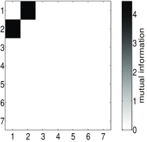
Figure 3: Test problem (C), with 7 input channels. Left panel: Averaged $\hat{I}(\hat{s}_{1}\ldots\hat{s}_{n})$ (k=3) from the output of FastICA hyvar2001 (parameters with lowest MI), JADE Cardoso93 , TDSEP (same parameters as in Meinecke02 ), and MILCA (k=30). The horizontal line indicates the true MI of the input channels. Right panel: Pairwise MI estimates $\hat{I}$ between all channel combinations, for the MILCA output components shown in Fig. 4 (diagonal is set to zero).

The aim of ICA is now to minimize $I(X_{1}\ldots X_{n})$ under a pure rotation R. Any rotation can be represented as a product of rotations which act only in some $2\times 2$ subspace, ${\bf R}=\prod_{i,j}{\bf R}_{ij}(\phi)$, where

$${\bf R}_{ij}(\phi)(x_{1}\ldots x_{i}\ldots x_{j}\ldots x_{n})=(x_{1}\ldots x_{i}^{\prime}\ldots x_{j}^{\prime}\ldots x_{n})$$ (17)

with

$$x_{i}^{\prime}=\cos\phi\;x_{i}+\sin\phi\;x_{j},\quad x_{j}^{\prime}=-\sin\phi\;x_{i}+\cos\phi\;x_{j}\;.$$ (18)

For such a rotation one has (see Eq.(10))

$$I({\bf R}_{ij}(\phi){\bf X})-I({\bf X})=I(X_{i}^{\prime},X_{j}^{\prime})-I(X_{i},X_{j})\;,$$ (19)

i.e., the change of $I(X_{1}\ldots X_{n})$ under any rotation can be computed by adding up changes of two-variable MIs. This is an important numerical simplification.

To find the optimal angle $\phi$ in a given $(i,j)$ plane, we calculated $\hat{I}_{ij}(\phi)=\hat{I}(X_{i}^{\prime},X_{j}^{\prime})$ for typically 150 different angles in the interval $[0,\pi/2]$, fitted these values by typically 3-15 Fourier components, and took then the minimum of the fit. The latter is useful because $\hat{I}(\phi)$ is not smooth in $\phi$, for essentially the same reasons as discussed in Learned . We also tried the augmentation proposed in Learned to smoothen $\hat{I}(X^{\prime},Y^{\prime})$. It worked equally well, by and large, as the Fourier filtering, but it was much slower.

Now the resulting MILCA-algorithm can be summarized:

1. Preprocess (center, filter, detrend, …) and whiten the data;

2. For each pair $(i,j)$ with $i,j=1\ldots n$ find the angle $\phi$ which minimizes a smooth fit to $\hat{I}_{ij}(\phi)=\hat{I}(X_{i}^{\prime},X_{j}^{\prime})$;

3. If $\hat{I}(X_{1}^{\prime}\ldots X_{n}^{\prime})$ has not yet converged, go back to step 2. Else, $\hat{s}_{i}=X_{i}^{\prime}$ are the estimates for the sources.

The order of choosing the sequence of pairs in point 2 is not essential. In our numerical simulations the convergence speed did not differ significantly whether we went through the pairs $(i,j)$ systematically or randomly.

III.2 Numerical Examples and Performance Tests

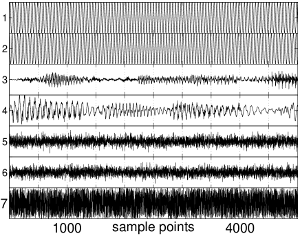
Figure 4: Seven output channels of the MILCA algorithm, test problem (C).

(A) As a first test we study the set of 18 problems proposed by Bach & Jordan Bach2002 and studied also in Learned . Each problem corresponds to a 1-d probability distribution $p(x)$. One thousand pairs of random numbers $x$ and $y$, each drawn iid from $p(x)p(y)$, are mixed as $x^{\prime}=x\cos\phi+y\sin\phi,y^{\prime}=-x\sin\phi+y\cos\phi$ with random angle $\phi$ common to all pairs (i.e., ${\bf A}$ is a pure rotation). Using MILCA, we obtained then the estimate $\hat{\bf A}$. This is repeated 100 times with different angles $\phi$ and with different random sets of pairs $(x,y)$. To assess the quality of the estimator $\hat{\bf A}$ (or, equivalently, of the back transformation $\hat{\bf W}=\hat{\bf A}^{-1}$), we use the Amari performance index $P_{err}$ Amari

$$P_{err}={1\over 2N}\sum_{i,j=1}^{N}({|p_{ij}|\over\max_{k}|p_{ik}|}+{|p_{ij}|\over\max_{k}|p_{kj}|})-1$$ (20)

where $p_{ij}=(\hat{\bf A}^{-1}{\bf A})_{ij}$.

Results are given in Table 1 (column ‘MILCA’) and compared there to the results of previous algorithms given in Learned . They are excellent in average and surpassed only by the RADICAL algorithm proposed in Learned which also uses an entropy estimate based on neighbor distances, but for the differential Shannon entropies $H(x^{\prime})$ and $H(y^{\prime})$. Another feature used in Learned is data augmentation: To obtain a more smooth dependence on the angle $\phi$, each data vector $(x,y)$ is replaced by an R-tuple (with $R=30$) of near-by points. The same augmentation trick can be used also for MILCA, and improves the results for very similar reasons. Indeed, our results obtained with MILCA and with data augmentation, given in the last column of Table 1, are even better than those of RADICAL. In the following tests we did not use data augmentation, because it is rather time consuming.

(B) As a second test we study an example taken from Meinecke02 . In involves five input sources (a sine wave, two different speech signals [the first half of “Houston, we have a problem” and “parental guidance is suggested” from audiosignal ], one white Gaussian noise, one uniformly distributed white noise) (5000 data points each) which are linearly mixed with a $5\times 5$ matrix A to form five output signals. In mixing these components, no time delay is used, i.e. the superpositions are strictly local in time. For this example it is possible to find the inverse transformation ${\bf W}={\bf A}^{-1}$ up to a permutation and up to scaling factors, because all sources are independent from each other and only one has a Gaussian distribution. To assess the quality of this back transformation we again use the Amari performance index.

The results obtained with two hundred different random mixtures of the sources (with uniformly distributed mixing matrices and with different realizations of the random channels for each mixture) are compared in the left panel of Fig. 2 with three standard algorithms: FastICA hyvar2001 , JADE Cardoso93 , and TDSEP Meinecke02 . We found that FastICA sometimes gets stuck in a local minimum, and runs differing only in the initial conditions can produce different results. The error bars shown in Fig. 2 indicate the resulting uncertainty of the performance measure, estimated from 20 realizations that differ only in initial conditions. The errors of JADE and FastICA are mainly due to their difficulty to separate one of the audio channels from the Gaussian noise. TDSEP is not able to decompose the two noise channels, since it is also not designed for this purpose (it uses time structures to separate signals). Very good results for all 200 mixtures are obtained by MILCA, although the audio signals are quit noisy and have nearly Gaussian distributions. The performance of JADE and FastICA compared to MILCA becomes better when the quality of the acoustic signals improves.

In addition to the Amari index, another (more direct) way to judge the accuracy of the source estimates is to look at the estimated MIs. If and only if the sources were estimated correctly, the MI should be zero. In the following we propose to use both the matrix of pairwise estimators $\hat{I}(\hat{s}_{i},\hat{s}_{j})$ and the estimated total MI $\hat{I}(\hat{s}_{1}\ldots\hat{s}_{n})$. The important advantage over the Amari index is that they can also be used when the exact sources are not known. Low values of the MI indicate that both the data is a mixture of independent components, and the separation algorithm worked well in producing some independent components. Notice that it cannot be expected in general that the components found are identical to the sources, e.g., if some of them are Gaussians. In Fig. 2 again MILCA shows the best performances.

Notice the very big difference between FastICA/JADE and TDSEP in the right panel of Fig. 2, which is much bigger than that measured with the Amari index. The first two have problems in separating one of the acoustic signals (signal #4 in Fig. 4) from the Gaussian, because it has a nearly Gaussian amplitude distribution, but for the same reason this is not punished by a large MI between the outputs (improved performance index see later in Fig. 14). TDSEP, using time information, has no problem with this, but cannot separate uniform from Gaussian noise – and is heavily punished for that by MI. In Sec. V we will show how to improve MILCA such that it can better separate components which have nearly Gaussian amplitude distributions but different time correlations. Using that improved MILCA will give much bigger performance difference with algorithms like FastICA/JADE.

(C) Next we want to investigate the case where the decomposition is neither perfectly nor uniquely possible. Such an example can be constructed by simply adding one cosine with the same frequency as the sine and one more Gaussian channel to the last test case. This now violates the assumption of independent sources, because the sine and cosine are strongly dependent. The theoretical value for the MI would be infinite, but a numerical estimator from a finite data sample gives a finite value, in our case $I(S_{1}\ldots S_{n})=0.72$ footnote3 . But for this example, perfect blind source separation is impossible also because the two Gaussians are not uniquely decomposable. We want to know how an ICA algorithm performs in view of such problems. It should still be able to separate those components which can be separated.

The total output MI is shown in the left panel of Fig. 3. We see that for all algorithms the MI is higher than the MI between the input channels, which serves essentially as a consistency test. The difference is smallest for MILCA. The MIs between all pairwise channel combinations obtained with MILCA are shown in the right panel of Fig. 3. They show again that MILCA has done a perfect job: All components are independent except for those which should not be. MILCA output is shown directly in Fig. 4. Although we do not show the input, it is clear that the separation has been as successful as possible.

(D) There are a number of blind source separation problems in the field of analytical spectroscopy, where quantitative spectral analysis of chemical mixtures is formulated as multivariate curve resolution (for recent reviews see smcr ; geladi2003 ; tauler2003 and as an ICA problem chemica ; epr ; chemica2004 ). Assuming Beer’s law, the spectrum of a mixture of pure constituents with spectra $s_{i}(\nu)$ and concentrations $A_{i}$ is $x(\nu)=\sum_{i}A_{i}s_{i}(\nu)$. Given a set of $N$ mixtures and $N$ pure components, we can then write this in vector notation as ${\bf x}(\nu)={\bf A}{\bf s}(\nu)$, analogous to Eq.(15). The task is to obtain estimates ${\bf\hat{s}}(\nu)$ for the pure components. This is the instantaneous linear ICA problem, except that in most applications of interest the spectral sources are not independent but have overlapping bands. This happens when chemical compounds in a mixture share several common or similar structural groups that demonstrate nearly the same spectral patterns.

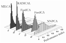
Figure 5: Performance index distributions over 7000 triples of three-component mixtures. For histograms (a),(b) the original spectra were decomposed, for (c)-(e) their second derivatives.

This difficulty makes mixture decomposition quite nontrivial for many BSS techniques used in chemometrics, unless interactive band selection (e.g. SIMPLISMA simplisma , IPCA ipca , BTEM btem ) is employed to avoid using those parts of the signals where severe overlaps reduce the quality of decomposition. Such preprocessing made by hand is, of course, a bit of an art, because these unsafe bands can not be known a priori in a blind problem. Since the focus here is rather on developing general purpose algorithms, we aim at using MILCA without interactive preprocessing in order to estimate its pure overall efficiency in cases when residual dependencies play a role.

To test the performance of MILCA on typical spectral data we collected a pool of 62 experimental molecular infrared absorption spectra in the range 550-3830 $cm^{-1}$ (822 data points each) taken from the NIST database nist . This test set was selected to contain organic compounds with common structural groups (benzene derivatives, phenols, alcohols, thiols) so that their spectra have multiple overlapping bands and, thereby, are mutually dependent. Then a sample of 7000 triples of three-component mixtures was constructed by choosing spectra randomly from the pool and applying random mixing matrices A footnote5 . For each decomposition the Amari performance index was computed. Fig. 5 compares its distributions for several different ICA algorithms including FastICA hyvar2001 , RADICAL Learned and Nonnegative PCA (NNPCA) nnpca . The latter uses the fact that pure spectra are non-negative and the same should hold for the estimates, so the nonnegativity is imposed as a soft constraint on the estimates ${\hat{s}_{\it i}}(\nu)$ in an optimization procedure. But our simulations showed that this constraint is often not fulfilled, and in some cases the output of NNPCA (as well as that of other algorithms) is negative. To a large part this is due to dependencies between the sources. Already prewhitening (i.e. PCA and rescaling) sometimes leads to decorrelated components which cannot be made nonnegative by any subsequent rotation. Trying to enforce nonnegativity neglecting other aspects might then be counterproductive, and this might partly explain the relatively poor performance of NNPCA (Fig. 5a).

NNPCA has to be applied to the original spectra, while it is well known that using derivatives of spectroscopic signals with respect to frequency can improve the results (see, e.g., chemica ; chemica2004 ). Taking such derivatives extracts the spectral information which is more independent between the sources Amaribook . In our numerical experiments, second order derivatives approximated by finite differences

$$\left.{d^{2}{\bf x}(\nu)\over d{\nu}^{2}}\right|_{{\nu}_{i}}\sim{\bf x}({\nu}_{i-1})-2{\bf x}({\nu}_{i})+{\bf x}({\nu}_{i+1}).$$ (21)

gave best performance footnote6 . This is clearly seen in the example of FastICA (compare distributions (b) and (c) on Fig. 5). But MILCA (e) and RADICAL (d) with second derivative data perform better than FastICA (c), and are almost equally good when compared to each other. Furthermore, our numerical results confirmed that nonnegativity is satisfied whenever the decomposition is successful (Amari index below 0.05) (see also the discussion in cich ). But whether this is fulfilled depends primarily on the dependencies between the original signals, and less on the algorithm employed.

A more detailed study of the potential of MILCA in multivariate spectral curve resolution will be given in a forthcoming publication astakh which will focus on the analysis of experimental mixtures and, in particular, on the comparison with recently developed interactive algorithms such as BTEM btem .

III.3 Reliability and Uniqueness of the ICA Output

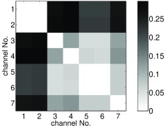
Figure 6: Square roots of variabilities ${\sigma_{ij}}$ of $I(R(X_{i},X_{j}))$ (with $k=6$) from MILCA output for test problem (C) (Fig. 4). Elements on the diagonal have been set to zero.

Obtaining the most independent components from a mixture is only the first part of an ICA analysis. Checking the actual dependencies between the obtained components should be the next task, although it is most often ignored. We have seen that it becomes easy and natural with MILCA, which was indeed one of our main motivations for MILCA. The next task after that is to check the reliability, uniqueness, and robustness of the decomposition. We have already discussed this in the last subsection for test example (C), but not very systematic. A systematic discussion will be given now.

Recently proposed reliability tests Meinecke02 ; noiseinj ; icasso are based on bootstrap methods or noise injection. We here present an alternative procedure which again makes use of the fact that MILCA gives reliable estimates of the actual (in-)dependencies: We test how much the estimated dependencies change under re-mixing the outputs.

In the simplest case, a multivariate signal with $n$ components is an instantaneous linear mixture of $n$ independent sources. This was the model we started with in subsection A. We assume it to apply when (i) all estimated pairwise MIs between all ICA components fall below a defined threshold, $\hat{I}(\hat{s}_{i},\hat{s}_{j})<D_{\rm max}$ for all $i,j=1,...,n$ and $i\neq j$, and (ii) the overall MI $\hat{I}(\hat{s}_{1}\ldots\hat{s}_{n})$ is below another threshold. Notice that the first criterion alone is not sufficient, see the appendix.

In real-world data, however, we are usually confronted with deviations from this simple model. The next simple possibility is that some pairwise MIs are still exactly zero, but others are not. Let us draw a graph where each of the $n$ output channels is represented by a vertex, and each pair $(i,j)$ of vertices is connected by an edge if $\hat{I}(\hat{s}_{i},\hat{s}_{j})>D_{\rm max}$. This gives a partitioning of the set of output components into connected clusters $C_{1},\ldots C_{m}$ with $m\leq n$. If, in addition, the MI between these clusters, $\hat{I}(C_{1},\ldots C_{m}$), is below another suitably chosen threshold, we consider each cluster to be independent (notice that we do not require all channels within a cluster to have a MI above the threshold $D_{\rm max}$). This is essentially our version of multidimensional ICA Cardoso98 . It uses exactly the same basic MILCA algorithm as defined above, and is thus much simpler conceptually than the ‘tree-dependent component analysis’ of Bach . Its main drawback is that it is not sensitive to the actual strengths of the non-zero interdependencies. A better algorithm which does take them into account will be discussed in Sec.IV.

In addition to this first step of an ICA output analysis, we have to test for the uniqueness of the components. For this purpose, we check whether the (one- or multi-dimensional) sources obtained by the ICA algorithm indeed correspond to distinct minima of the contrast function or whether other linear combinations exist which show approximately the same overall dependencies. An example for the latter case is given by two uncorrelated Gaussian signals. They remain independent under rotation foot7 .

A good estimator for the uniqueness of the ICA output is the variability of the pairwise MI under remixing, i.e. under rotations in the two-dimensional plane:

$$\sigma_{ij}=\overline{I(X_{i},X_{j})}-\hat{I}_{ij}(\phi_{\rm min})\quad{\rm for}\;\;i\neq j$$ (22)

where the global minimum of $\hat{I}$ is at $\phi=\phi_{\rm min}$, and

$$\overline{I(X_{i},X_{j})}={2\over\pi}\int_{0}^{\pi/2}d\phi\;\hat{I}_{ij}(\phi)$$ (23)

(notice that $I_{ij}(\phi)$ is periodic in $\phi$ with period $\pi/2$). For unique solutions the MI will change significantly (large $\sigma_{ij}$), but it will stay almost constant for ambiguous outputs (small $\sigma_{ij}$).

Results for the MILCA output of test problem (C) are shown in Fig. 6. (to aid in the interpretation, the actual output signals were shown in Fig. 4). The basic ICA model is violated both in the Gaussian noise subspace and the $sin/cos$ subspace. In the Gaussian subspace the components are independent, but it should be impossible to find a unique decomposition. Indeed, $\sigma_{5,6}\approx 0$ (Fig 6) and $\hat{I}_{5,6}\approx 0$ (Fig. 3). For the dependent components ($sin/cos$ subspace) the situation is different. We expect to have $\sigma=0$ also here, corresponding to the isotropy of the distribution in this subspace. But $\hat{I}$ should be much larger than zero, because the two signals are not independent. Indeed, we see $\sigma_{1,2}\approx 0$ and $\hat{I}_{1,2}\gg 0$. In general, it depends on the specific application whether one should attribute any meaning to $\sigma_{ij}$ when components $i$ and $j$ are not independent. Finally, we conclude from Fig. 3(right) and Fig. 6 that the channels 3, 4 (audio signals), and 7 (uniformly distributed noise) are one dimensional sources, because they are independent from any channel, $\hat{I}_{3,i}\approx\hat{I}_{4,i}\approx\hat{I}_{7,i}\approx 0$, and are reliable, $\sigma_{3,i}\approx\sigma_{4,i}\approx\sigma_{7,i}\gg 0$.

Figure 7: Unsmoothened estimates of $\hat{I}(\phi)$ for two randomly mixed uniform distributions, corrupted with isotropic Gaussian measurement noises with different signal-to-noise ratios $SNR=\infty,13,7,4,1$ (from top to bottom), plotted against $\phi$.

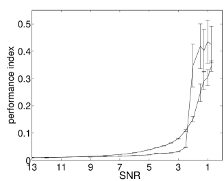
Figure 8: Averaged Amari index against the signal-to-noise ratio. The condition number of the mixing matrices is 6. The upper curve (in the SNR range from 7 to 3) is for standard MILCA, the lower for n-MILCA.

III.4 Noisy Signals

Because our aim is to apply MILCA to real world data, we have to discuss the influence of measurement noise. In the literature there exist several algorithms which are specially tailored to this problem (see e.g. Ref. hyvar2001 , chapter 15). Typically, in order to obtain optimal performance, the noise is assumed to satisfy very special properties like being additive, uncorrelated, isotropic and Gaussian. Below we will present a modified MILCA algorithm which assumes that we have measurement noise with exactly these properties.

Alternatively, one can take just a standard ICA algorithm (in our case MILCA as described above), and analyze how its output depends on the noise level. In the following we will compare both approaches.

We start with two uniformly distributed variables and mixed them with a random $2\times 2$ matrix with a fixed condition number. After that, iid Gaussian noises are added to each of the two mixtures. The amplitudes in both channels are the same,

$$x_{i}(t)=\sum_{j=1}^{2}A_{ij}s_{j}(t)+\eta_{i}(t)$$ (24)

with $\langle\eta_{i}(t)\eta_{j}(t^{\prime})\rangle=r\delta_{ij}\delta_{tt^{\prime}}$. For the case were we do not use any information of the measurement noise signals $x_{i}(t)$ are then simply used as input in MILCA. In Fig. 7 we show $\hat{I}(\phi)$ for the same mixing matrix but different signal-to-noise ratios $SNR={\rm var}(s_{i}(t))/r$. We see that $\hat{I}$ becomes flatter (the variability with respect to the mixing angle decreases) with decreasing SNR footnote . The presence of noise leads also to a shift of the minimum. Both effects introduce errors in estimating the original mixing matrix. The upper curve in Fig. 8 shows the averaged Amari index over 100 realizations with different noise and mixing matrices.

To reduce this error we modify MILCA to n-MILCA (noisy MILCA). At first we do a ’quasiwhitening’ with the estimated covariance matrix ${\bf V}=({\bf C}_{x}-r\bf{1})^{-1/2}$ of the pure signals (see, e.g., hyvar2001 , chapter 15) to decorrelate the original sources. As a consequence of this, the noise will become now correlated, and with it also the entire ’quasiwhitened’ signal. Because of this we should not minimize $\hat{I}(\phi)$, since in this way we would introduce a bias as seen in Fig. 7 towards wrong values of $\phi$. Instead we minimize $\hat{I}(\phi)+{1\over 2}\log(1-C_{ij}(\phi)^{2})$ where we have subtracted the ‘linear’ contribution (see Eq.(7)). In Fig. 8 we show again the averaged Amari index for the same realizations as used before. Making use of detailed information on the noise clearly improved the results, except for very small SNR. The amount by which it improves depends on the condition number of the mixing matrix. For matrices far away from singularity (low condition number) the quasiwhitening has little effect and there is hardly any difference, while for large condition numbers the two mixtures are nearly the same and it is impossible to obtain good results with either algorithms.

Finally, before leaving this subsection, let us say a few words about outliers. Outliers are just a special case of noise. Because our MI estimator is based on the k-nearest neighbor distribution, outliers make less difficulties Ref.Learned than e.g. in kurtosis based algorithms.

III.5 A Real-World Application

Finally, let us apply MILCA to a fetal ECG recording from the abdomen and thorax of a pregnant woman (8 electrodes, 500 Hz, 5 seconds). We chose this data set because it was analyzed several times with different ICA algorithms Lath ; Cardoso98 ; Meinecke02 ; alex and is available on the web ECGdata .

The output components of MILCA are shown in Fig. 9 footnote1 . We used $k=30$ neighbors for estimating MI, and to obtain the minima of $\hat{I}_{ij}(\phi)$ we fitted with 3 Fourier components. The success of the decomposition is already seen by visual inspection. Obviously, channels 1-2 are dominated by the heartbeat of the mother, and channel 5 by that of the child. Channels 3, 4, and 6 still contain heartbeat components (of mother and child, respectively), but look much more noisy. Channels 7 and 8 seem to be dominated by noise, but with rather different spectral compositions.

In order to verify this also formally (which would be essential in any automatic real-time implementation) we first show in Fig. 10 (left panel) the pairwise MIs. We see that most MIs are indeed small, except the one between the first two components. This indicates again that the first two components belong to the same source, namely the heart of the mother. But some of the other MIs seem to be definitely non-zero, even if they are small. This indicates that the decomposition is not perfect, as is also seen by closer inspection of Fig. 9.

Finally, we show in the right panel of Fig. 10 the variabilities under re-mixing. They confirm our previous findings. In contrast to the sine/cosine pair in test example (C), the first two components have non-zero $\sigma$, showing that the distribution in this subspace is not isotropic and that one can minimize the interdependence in it by a suitably chosen demixing. Apart from that, the biggest values of $\sigma$ are for channels 1, 2, and 5, showing that these channels are most reliably and uniquely reconstructed. They are just the channels dominated most strongly by heart beat.

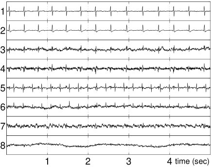
Figure 9: MILCA output: components after minimizing $I(X_{1}\ldots X_{8})$ for the heart beat example of Sec. III.E.

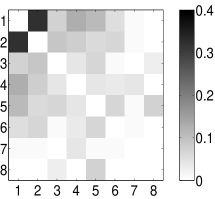
Figure 10: Left panel: $\hat{I}$ between all the pairwise combinations of the signals shown in Fig. 9. Right panel: Square roots of variabilities $\sigma_{ij}$ of $\hat{I}_{ij}(\phi)$. In both panels the values on the diagonal are set to zero.

IV Cluster Analysis

We pointed already out that the usual assumption of independent one-dimensional sources as in Eq.(15) is often unrealistic. Take e.g. the ECG discussed in the previous subsection, and assume that both hearts – the one of the mother and the one of the fetus – are independent chaotic dynamical systems. A chaotic system with continuous time must have at least 3 excited degrees of freedom ott . With any generic placement of the electrodes, we should then expect to pick up $\geq 3$ different components from each heart. These components must be strongly dependent on each other, even after having been whitened broomhead . Thus each heart must contribute to at least 3 output components in any linear ICA scheme. For the mother heart we have indeed found 2 components. The fact that we have not clearly identified more dependent components in the output should be considered as failure of the instantaneous linear algorithm and will be dealt with more systematically in Sec. V.

In any case, in view of this we have to expect that outputs in real-world applications are not independent but come in connected clusters. Moreover, we should expect that even within one cluster there are more or less strongly connected substructures. We have already discussed in Sec. III.c a simple way how to identify these clusters. In the present section we present a more systematic analysis.

Figure 11: Dendrogram for Fig. 9. The height of each cluster $(ij)$ corresponds to $\hat{I}(X_{i},X_{j})$ ($k$=6).

Our strategy is to estimate a proximity matrix from the MIs, and then to use a hierarchical clustering algorithm to obtain a dendrogram. No thresholds are used in constructing the dendrogram, i.e. it is constructed without making any decision about which MILCA output channels are independent or not. Only after its construction we decide, usually on heuristic reasons and based on arguments of practicality and usefulness, which channels are actually grouped together. This is more convenient, usually, than the algorithms of Bach ; phinv ; topica where this decision stands at the starting point of the algorithm or is an essential part of it.

A first technical problem concerns the choice of the proximity matrix. One might be tempted to use MI directly. But we want to include the possibility that some of the channels to be grouped together are already multidimensional by themselves. In this case, using MI would introduce a bias: multivariate channels not only tend to carry more information than univariate ones, they also will have larger MIs. Therefore we propose to use as a similarity measure alex2

$$P_{ij}={\hat{I}(\hat{s}_{i},\hat{s}_{j})\over\dim(\hat{s}_{i})+\dim(\hat{s}_{j})},$$ (25)

where $\dim(x)$ is the dimension of the variable $x$, i.e. the number of its components.

In most cluster algorithms the proximity matrix P is used only for the first step. In the subsequent steps, proximities for clusters are derived from it in some recursive way jain-dubes . In the present paper we propose to use ‘MI-based Clustering’ (MIC) alex2 which is based on the grouping property Eq.(9). Thus, a cluster of output channels is just characterized by the multivariate signal formed by the tuple of its individual channels, and the proximity measure is still given precisely by Eq.(25) at each level of the hierarchy.

In summary, our cluster algorithm is as follows. We start with $n$ (usually univariate) MILCA output channels $\hat{s}_{i}\;,\;\;i=1,\ldots n$, and we compute $P_{ij}$ according to Eq.(25). After that, we enter the following recursion:

1. Find the pair with minimum distance in the matrix, say clusters $i$ and $j$;

2. Combine the clusters $i$ and $j$ to a new cluster $(ij)$ with multivariate data $\hat{s}_{ij}$, and attribute to it a height $\hat{I}(\hat{s}_{i},\hat{s}_{j})$ in the dendrogram. Thereby the total number of clusters is reduced by one, $n\leftarrow n-1$;

3. If the new value of $n$ is 1 then exit; else

4. update the proximity matrix $P_{ij}$ and go to 1.

The dendrogram obtained in this way for the ECG data of Sec. III.E is shown in Fig. 11. In this figure two clusters are clearly distinguishable, the mother cluster containing channels (1, 2, 3, 4, 7) and the fetus cluster formed by channels 5 and 6. This agrees perfectly with the interpretation given in Sec. III.E. One can of course debate whether, e.g., channel 7 belongs to the mother cluster or not, but this can be decided as it seems most convenient, and it will in general have little effect on any conclusions. One way to make use of such a clustering is in cleaning the data and separating the individual sources. For that, one prunes everything except the wanted cluster, and reconstructs the original channels by applying the inverse of the matrix $\bf W$. Results obtained in this way will be shown in the next section, after having discussed how to take into account temporal structures.

V Using Temporal Structures

V.1 Instantaneous Demixing that Minimizes Delayed Mutual Informations

Until now we have not used any time structure in the signals. In the following we shall assume the signals to be stationary with finite autocorrelation times. ICA-algorithms in the literature either use no time information at all (JADECardoso93 , FastICAhyvar2001 , INFOMAXbell , …) or, if they do use it, they use only second order statistics (AMUSE tong , TDSEP Meinecke02 ,…). The first group is not able to decompose two Gaussian signals with different spectra, while the second group is not able to separate two temporally white signals with different amplitude distributions. Obviously one has to make use of time structure and higher order statistics, to obtain optimal results in general mueller ; Amaribook . This is precisely what we will do in this subsection.

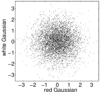
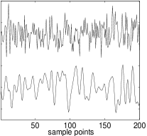
Figure 12: Left panel: scatter plot of the two Gaussian sources with different spectra. Right panel: Output of the modified MILCA algorithm ($\tau=1$ and $m=2$), where white Gaussian is on top and red Gaussian is on bottom.

Figure 13: Change of $\hat{I}$ under rotation, for the Gaussian model shown in Fig. 12. The nearly horizontal curve shows the behavior without, the sinusoidal one the result with using delay embedding. Here the actual mixing angle is $0$.

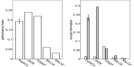
Figure 14: Test problem (B) of Sec.III, consisting of 5 input channels (compare with Fig.2). Algorithm “MILCA^∗” now refers to the minimization of Eq.(28). The gray bars on the right panel show the full MI given in Eq.(28). The embedding parameters are $m=2$, $\tau=1$.

Normally the first step in nonlinear time series analysis of univariate signals is delay embedding Kantz : One constructs a formally $m$-variate signal, for any $m>1$, by simply forming $m$-dimensional ‘delay vectors’ with a suitably chosen delay $\tau$,

$${\bf x}(t)=[x(t-\tau),x(t-2\tau),\ldots x(t-m\tau)]^{T}.$$ (26)

Thus one characterizes the “state” of a signal at time $t$ by giving not its value at $t$ itself, but at $m$ previous times. This makes of course sense only when there is any time structure in the signal. Similarly we can also embed multivariate signals. For $n$ measured channels one obtains thereby an $n\times m$ ‘delay matrix’

$${\bf X}(t)=[{\bf x}_{1}(t),\ldots{\bf x}_{n}(t)].$$ (27)

To decompose an instantaneous linear mixture of $n$ signals with either non-Gaussian statistics or with non-trivial time structure, we propose to simply minimize the MI,

$$\hat{I}({\bf s}_{1}(t),\ldots{\bf s}_{n}(t))\stackrel{{\scriptstyle!}}{{=}}\min.$$ (28)

Notice that we have here considered the delay vectors as joint entities, i.e. we do not include in Eq.(28) the MIs between the different delays of the same $x_{i}$. More explicitly footnote4 ,

$$I({\bf x}_{1}(t),\ldots{\bf x}_{n}(t)) = I(x_{1}(t-\tau),\ldots x_{1}(t-m\tau),$$

$$x_{2}(t-\tau),\ldots x_{2}(t-m\tau),\ldots$$

$$x_{n}(t-\tau),\ldots x_{n}(t-m\tau))$$

$$- \sum_{i=1}^{n}I(x_{i}(t-\tau),\ldots x_{i}(t-m\tau))$$

$$= \sum_{i=1}^{n}H({\bf x}_{i}(t))-H({\bf x}_{1}(t),\ldots{\bf x}_{n}(t))$$

To minimize this, we proceed again as in Sec.III, i.e. we decompose the rotation needed to minimize $\hat{I}({\bf x}_{1}(t),\ldots{\bf x}_{n}(t))$ into rotations within each of the $n(n-1)/2$ coordinate planes. Each of the latter rotations still involves rotations of $m$ delay coordinate pairs, but this can be further decomposed into $m$ rotations where only one delay coordinate pair is rotated. We thereby obtain

$$I(\ldots{\bf x}_{i}^{\prime}(t),\ldots{\bf x}_{j}^{\prime}(t)\ldots)-I(\ldots{\bf x}_{i}(t),\ldots{\bf x}_{j}(t)\ldots)$$

$$=I({\bf x}_{i}^{\prime}(t),{\bf x}_{j}^{\prime}(t))-I({\bf x}_{i}(t),{\bf x}_{j}(t))$$

$$=\;I(x_{i}(t-\tau),\ldots x_{i}(t-m\tau))$$

$$\;\;+I(x_{j}(t-\tau),\ldots x_{j}(t-m\tau))$$

$$\;\;-I(x^{\prime}_{i}(t-\tau),\ldots x^{\prime}_{i}(t-m\tau))$$

$$\;\;-I(x^{\prime}_{j}(t-\tau),\ldots x^{\prime}_{j}(t-m\tau))$$

$$\;\;+m\;[I(x^{\prime}_{i}(t),x^{\prime}_{j}(t))-I(x_{i}(t),x_{j}(t))]\;,$$ (30)

where we have used in the last term the fact that $I(x^{\prime}_{i}(t),x^{\prime}_{j}(t))$ is independent of $t$ due to stationarity. If $m=2$, this is again a sum of pairwise MIs. If $m>2$, we have to estimate $m$-dimensional MIs directly.

To illustrate this on a simple example, let us assume two channels where $x_{1}(t)$ and $x_{2}(t)$ are instantaneous mixtures of two Gaussian signals with the same amplitude distribution but with different spectra: $x_{1}$ is white (iid), while $x_{2}$ is red and was obtained by filtering with a Butterworth filter of order 6 and with cutoff frequency 0.3. For simplicity we assume the mixing to be a pure rotation. Then a scatter plot of the vectors $(x_{1}(t),x_{2}(t))$ is completely featureless, see Fig. 12(left), and will not allow a unique decomposition. But using delay embedding with $m=2$ is sufficient to obtain the original sources (Fig. 12, right panel).

Figure 15: Upper panel: Two channels of the ECG of a pregnant woman. Lower panel: MILCA output from these two channels.

Figure 16: MILCA output from the delay embedded two channel ECG with embedding dimension $m=3$.

Similarly good results were obtained with the less trivial examples of previous sections. In particular, we tested the algorithm on test problem (B) of Sec. III.B (Fig. 14). The performance of MILCA is improved substantially, even with $m=2$. The delayed MI (Eq.(28)) which make use of the time structure serves as a better performance value (Fig. 14 (right)). Now JADE and FastICA are also heavily punished for not separating one audio signal from Gaussian noise (as one can see the MI for TDSEP is nearly unchanged because the time correlation in the output is minimal).

V.2 Demixing with Delays

The most general linear demixing ansatz for a stationary system assumes superpositions of the observed signals with delays. Using up to $m$ delays $\tau,2\tau,\ldots m\tau$, we thus make the ansatz (see e.g. Ref. hyvar2001 , chapter 19)

$$\hat{s}_{i}(t) = \sum_{j=1}^{N}\sum_{k=1}^{m}w_{ij}^{k}\;x_{j}(t-k\tau)$$ (31)

$$= \sum_{j=1}^{N}{\bf w}_{ij}{\bf x}_{j}(t)\;,$$

where ${\bf x}_{j}(t)$ is a delay vector as defined in Eq.(26) and

$${\bf w}_{ij}=[w_{ij}^{1}\ldots w_{ij}^{k}].$$ (32)

Since we have now linear superpositions of $n\times m$ measurements $x_{j}(t-k\tau)$ on the right hand side, we can also determine the same number of $\hat{s}_{i}(t)$ for each value of $t$, i.e. the index $i$ in Eq.(31) runs from 1 to $nm$.

This ansatz is obviously more appropriate than instantaneous mixing, if the signals $x_{i}(t)$ are themselves superpositions of delayed sources. If they involve a finite number of delays,

$$x_{i}(t)=\sum_{j}\sum_{k=1}^{m^{\prime}}a_{ij}^{k}s_{j}(t-k\tau),$$ (33)

Eq.(31) with finite $m$ would not give the exact demixing, since inverting Eq.(33) would require an infinite number of delay terms. Also, Eq.(31) in general does not correspond to the inverse of Eq.(33), because its solutions are in general not components of any delay vectors. But it should definitely be a better ansatz than the instantaneous Eq.(15).

Apart from that, we would anyhow not expect Eq.(33) to be the correct model in most applications. The main reason why we believe that Eq.(31) is useful in many applications is that it can cope much better with the situation discussed at the beginning of Sec. IV. Assume for the moment that there is a single source. Different sensors (as, e.g., different ECG contacts) typically see different projections of this source, and the signals $x_{i}(t)$ can therefore be considered as different coordinates describing its dynamics. As pointed out by Takens Kantz , delayed values of one single signal can also be considered as different coordinates. Our demixing ansatz basically reflects the hope that suitable superpositions of delayed values of $x_{i}$, say, can mimic any other signal $x_{j}$.

To illustrate this, we consider again the above ECG recording. We assume for the moment that only the two channels with the most pronounced fetus heartbeat are available and try to decompose them into mother and fetus heartbeat. These two channels are shown in Fig. 15 (top). They are still dominated by the mother heartbeat. But the R peak of the mother has a very different shape in both channels: In the lower trace it is mainly positive, while it has both positive and negative components in the upper. It is therefore clear that there cannot exist an instantaneous superposition to which the mother’s heartbeat does not contribute. Instantaneous ICA must fail for this case, as is indeed seen in the lower two traces of Fig. 15.

In order to obtain the least dependent components obtainable with Eq.(31), we minimize again the MI. But now, in contrast to the previous subsection, the output variable $s_{i}(t)$ are not delay coordinates of any sources, and therefore we must minimize the full MI between all $s_{i}(t)$,

$$\hat{I}(s_{1}(t),\ldots s_{nm}(t))\stackrel{{\scriptstyle!}}{{=}}\min.$$ (34)

The minimization is done again, as in all previous cases, by performing successive transformations in 2-dimensional subspaces and by using Eq.(10). In terms of the actual algorithm, the only difference to the previous subsection is that we now make rotations in all subspaces.

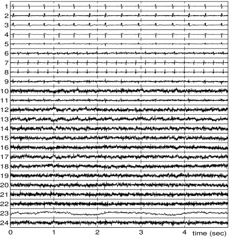
Figure 17: MILCA output from the embedded eight channel ECG (k=100, m=3)

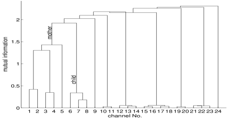
Figure 18: Dendrogram for Fig. 17. Heights of each cluster correspond to $I(X_{i},X_{j})$ of the cluster $ij$ ($k$=3).

In our application to the fetal ECG we use embedding dimension $m=3$ and the smallest possible delay, $\tau=1/500\;{\rm s}^{-1}$. Results for the two channels shown in Fig. 15 are now shown in Fig. 16. The separation is now improved. Although we still have one output channel where mother and fetus are strongly mixed (channel #4), channel #6 is now practically pure fetal heartbeat.

Finally, we applied this method to all 8 channels of the ECG. Using again $m=3$ gives altogether 24 output channels. They are shown in (Fig. 17), and we can clearly see which ones are dominated by the mother heartbeat, which by the fetus, and which by noise. In order to do this more objectively, we again apply the cluster algorithm of Sec. IV, with the result shown in Fig. 18. There one can clearly see two big clusters corresponding to the mother and to the fetus. There are also some small clusters which should be considered as noise.

For any two clusters (tuples) $X=X_{1}\ldots X_{p}$ and $Y=Y_{1}\ldots Y_{q}$ one has $I(X_{1},\ldots Y_{q})\geq I(X)+I(Y)$. This guarantees, if the MI is estimated correctly, that the tree is drawn properly, i.e. each parent node is above the two daughter nods. The two slight glitches (when clusters (1 - 14) and (15 - 18) join, and when (21 -22) is joined with 23) result from small errors in estimating MI. They do not affect our conclusions.

In Fig. 19 we show the matrices of pairwise MIs (left panel) and of pairwise variabilities (right). They are as expected, and they show much more pronounced structures than the matrices without delay embedding (Fig. 10). For the MIs one can see a clear block structure, i.e. the mother and fetus components are now indeed more independent, as suggested also from the traces themselves. From the right panel we see that the main mother channels (1-4) and the fetus channels (7-8) are very stable. The rest is mostly noise, and is not stable as indicated by the very small variabilities.

The final result of MILCA is obtained by pruning everything not belonging to the cluster of interest,

$$\hat{s}_{i}(t)\to{\cal P}_{C}\;\hat{s}_{i}(t)\equiv\left\{\begin{array}[]{rl}\hat{s}_{i}(t)&\qquad i\in{\rm cluster}\;\;C\\ 0&\qquad{\rm else}\end{array}\right.$$ (35)

and performing the back transformation. At this stage there arises the problem that the reconstructed signals

$$\hat{x}_{j,k}(t;C)={\bf W}^{-1}_{(j,k),i}{\cal P}_{C}\;\hat{s}_{i}(t)\;,\quad{\bf W}_{i,(j,k)}=w^{k}_{ij}$$ (36)

are in general not delay vectors, i.e.

$$\hat{x}_{j,k+1}(t;C)\neq\hat{x}_{j,k}(t-\tau;C)\;.$$ (37)

In view of this, one has to make some heuristic decision what to use as a cleaned signal. We use simple averages,

$$\hat{x}_{j}(t;C)={1\over m}\sum_{k=1}^{m}\hat{x}_{j,k}(t+k\tau;C)\;.$$ (38)

We do not show all 8 full traces for the mother and fetus, because this would not be very informative: The results are too clean to be judged on this scale. Instead we show in Fig. 20 blow-ups of one of the original traces and the contributions to it from the mother and from the fetus. The separation is practically perfect.

Before leaving this section, we should point out that one can, in principle, also construct algorithms in between those of the last two subsections. In subsection A we had used delays to minimize the lagged MI, but we had not used the delays in the demixing. In the present subsection, we have used the same delays both for minimizing MI and for demixing. A generalization consists in using $m$ delays in the demixing, but minimizing the MI with additional $m^{\prime}$ delays. Thus we make the same demixing ansatz Eq.(31) as above, but we minimize

$$\hat{I}({\bf s}_{1}(t),\ldots{\bf s}_{nm}(t))\stackrel{{\scriptstyle!}}{{=}}\min.$$ (39)

where we have used the definition of $I({\bf s}_{1}(t),\ldots)$ given in Eq.(V.1), and $\hat{\bf s}_{i}(t)=[\hat{\bf s}_{i}(t-\tau),\hat{\bf s}_{i}(t-2\tau),\ldots\hat{\bf s}_{i}(t-m^{\prime}\tau)]^{T}$. Up to now, we have not yet applied this to any problem.

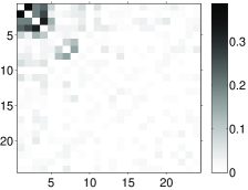
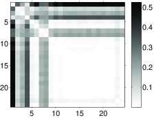
Figure 19: Left panel: Pairwise MIs between the estimated components shown in Fig. 17. Right: Square roots of variabilities ${\sigma_{ij}}$ of $I(X_{i},X_{j})$ (with $k=6$). Elements on the diagonal have been set to zero.

Figure 20: Short segment from the original ECG (a), of the mother and fetus contributions estimated without delay embedding (b,c), and of the two contributions estimated with delay embedding (d,e).

VI Discussion

There is by now a huge literature on independent component analysis. Therefore, most of our treatment is related in some form to previous work. One of our basic premises was that we did not so much care about speed, but we wanted as precise a dependency measure as possible. Our claim that this is provided in principle by MI is of course not new. But we believe that our estimator via $k$-nearest neighbor statistics is new and provides the most precise mutual information estimate. It is closely related to similar estimators for differential entropies which had been used in Pham ; Learned , and the quality of our results in the most simple 2-d blind source separation problem is very similar to the one in Learned . The main virtue of our MI estimator, compared to all previous MI estimators, is the numerical fact that it becomes unbiased when the two distributions are independent.

While using differential entropies instead of MI would give the same quality and somewhat simpler codes for the basic blind separation problem, using MI has other advantages: with it we can estimate the residual dependencies between the output components. Our use of this knowledge for estimating the output uniqueness and robustness, by measuring how the dependencies change under re-mixing, seems to be new. Previous authors used for this problem resamplings and/or noise addition Meinecke02 ; noiseinj ; icasso .

In addition to this, we used the MIs between the outputs to cluster them, and we then used this clustering to obtain the contributions of the individual (multidimensional) sources to the measured signals. The observation that “independent” component analysis will in general, when applied to real world data, not give independent components is not new either Bach ; topica ; Cardoso98 . We stress it by calling our approach a “least dependent” component analysis. Our detailed implementation of this idea seems to be new, not the least because our clustering algorithm is novel and uses a specific property of MI not shared by other contrast functions.

Although the extension of our algorithm to data with time structure discussed in Sec.V.A seems straightforward, this strategy of combining in the contrast function deviations from Gaussianity both at equal times and at non-equal times has been considered in very few papers only mueller ; Amaribook . The present paper is the first which uses directly MI for combining these two aspects. In Sec. V. was shown that this can substantially improve the separation e.g. of audio signals.

Both the ansatz of Sec.V.A and the method of demixing with delays in Sec.V.B are entirely based on MI, and use essentially the same algorithm. Therefore, also the generalization mentioned at the end of Sec.V.B uses essentially the same basic algorithm. This last generalization was never considered before, but demixing with delays is of course a very widely treated concept (see e.g. hyvar2001 ). It is usually called ‘convolutive mixing’. In our presentation we stressed several features which are typically overlooked. One is that the ‘convolutive’ demixing ansatz Eq.(31) is in general, when the sources $s_{i}(t)$ are not strictly independent, not equivalent to a convolutive mixing ansatz, because the sources then will not be components of delay vectors. This is also the reason why we avoided the term ‘convolutive mixing’.

Just as ICA may be considered as a generalization of principle component analysis (PCA) to non-Gaussian contrast functions, mixing with delays is a generalization of multivariate singular source analysis (SSA) kepenne ; ghil to include non-Gaussianity. Univariate SSA, see e.g. broomhead ; vautard , is often considered as an alternative to Fourier decomposition and has found many applications, while multivariate SSA was mainly used in geophysics. Indeed, we consider blind source separation algorithms based on temporal second order statistics (AMUSE, TDSEP) as more closely related to multivariate SSA than to other ICA methods based on nonlinear contrast functions.

While we discussed also a number of other applications and test models, our main test problem was the ECG of a pregnant woman, and the task was mainly to extract a clean fetal ECG. We have chosen this partly because this ECG was already used in previous ICA analyses Lath ; Cardoso98 ; Meinecke02 . We believe that our method clearly outperformed these and gives nearly perfect results, although we should admit that the signals to start with were already exceptionally clean. It would be of interest to see how our method performs on more noisy (and thus more typical) ECGs. Obtaining fetal ECGs should be of considerable clinical interest, although it is not practiced at presence, mainly because of the formidable difficulties to extract them with previous methods. In this respect we should mention the seminal work of kaplan ; richter where fetal ECGs were extracted even from univariate signals using locally nonlinear methods. It would be interesting to see how our method compares with such a nonlinear method when the latter is used for multivariate signals.

Throughout the paper, we used total MI as a contrast function. One might a priori think that the sum of all pairwise MIs would be easier to estimate, and could be as useful as the total MI. Neither is true. One reason for the efficiency of our algorithm is that changes of the total MI under linear remixings can be estimated by computing only pairwise MIs (except for the method of Sec. V.A with embedding dimension $m>2$). Thus one needs to compute the full high-dimensional MI only once. For all changes during the minimization, computing pairwise MIs is sufficient. But this does not mean that total MI is essentially a sum of pairwise MIs. We showed in the appendix that this can be very wrong. And we found in more realistic applications that the sum over all pairwise MIs sometimes increases when we minimize total MI. Therefore we consider the sum over all pairwise MIs as a very bad contrast function.

This is somewhat surprising if one considers ICA as a generalization of PCA. PCA can be viewed as minimalization of the sum over all squared pairwise covariances. But we believe that this close relation between ICA and PCA is somewhat misleading anyhow. It is usually based on this analogy that the data are first pre-whitened, before the ICA analysis proper is made, which is then restricted to pure rotations. We showed by means of a counter example that this can lead to a solution which does not have minimal MI. This was a rather artificial example, and the problem might not be serious in practice (all our results were obtained, for simplicity, with prewhitening). But one should keep it in mind in future applications.

Finally we should point out that Eqs. (9,10) hold for the exact MI, but are only approximately true for our estimators. Therefore, working directly on higher dimensional MIs, without breaking their changes down to 2-dimensional contributions, can give slightly different results. We found no big systematic trends, although we expect in general that estimates using the smallest dimensions are most reliable. The reason is that they are based on smaller distances for fixed $k$, or use larger $k$ when using the same distances. The first reduces systematic errors, the second statistical ones. The decrease in CPU time when using Eq. (10) to decrease the effective dimensionality is a further important point.

VII Conclusion

In the first part of the paper we discussed the classical linear instantaneous ICA model and introduced a new algorithm which shows better results than conventional ICA-algorithms. Our algorithm should be particularly useful for real world data, since it works with actual dependencies between reconstructed sources (as measured by mutual informations), and thus easily allows to study the question how independent and unique are the found components.

In the following we discussed the case where outputs can be grouped together for a meaningful interpretation. We again saw that MI has some properties which makes it the ideal contrast function, also for this purpose.

Finally, when we included time domain structures, we again could use the same estimates of MI, with basically the same algorithms. This – and the excellent results when applied to a fetal electrocardiogram – suggest that our method of basing independent component analysis systematically on highly precise estimates of MI is very promising. It is true that our method is slower than existing algorithms like FastICA or JADE, but we believe that the improved results justify this effort in many situations, in particular in view of the ever-increasing power of digital computers.

The software implementation of the MILCA algorithm is freely available online online .

Appendix

In this appendix we give two counter examples showing somewhat counterintuitive features of the MI. In the first example we have two continuous variables, and the joint density is constant in an L-shaped domain

$$D=\{[0,l_{x}]\times[0,\epsilon]\cup[0,\epsilon]\times[0,l_{y}]\}.$$ (40)

It is zero outside $D$. It is easily seen that $I(X,Y)\to h$ in the limit $\epsilon\to 0$, with $h=p\log p+(1-p)\log(1-p)$ and with $p=l_{x}/(l_{x}+l_{y})$. In this limit, the marginal distributions are superpositions of a delta peak at $x$ or $y$ equal to zero, and a uniform distribution on $[0,1]$. The components have relative weights $l_{x}:l_{y}$. The only information about $y$ learned by fixing $x$ is on which arm the pair $(x,y)$ is located, and for this $h$ bits are sufficient.

On the other hand, any linear transformation applied to the $(x,y)$-plane would give an L-shaped figure with at least one oblique arm. For such a distribution knowing $x$ would specify $y$ with an accuracy $\sim\epsilon$, and thus $I(X,Y)\sim-\log\epsilon\to\infty$ for $\epsilon\to 0$. But the covariance between $X$ and $Y$ is not zero, hence the minimal MI is reached (for small $\epsilon$) when the correlation coefficient $r$ is non-zero. A more detailed analysis shows that $I(X,Y)$ of the distribution rotated by an angle $\phi$ is not symmetric under $\phi\to-\phi$, if $l_{x}\neq l_{y}$.

The second example is one of three random variables $X,Y$, and $Z$ which are pairwise strictly independent, but globally dependent. For simplicity, the example uses discrete and indeed binary variables. We have thus 8 probabilities $p(x,y,z)$ for each variable being either 0 or 1, and we chose them as $p(0,0,0)=p(1,1,0)=p(0,1,1)=p(1,0,1)=1/8+\epsilon$ and $p(0,0,1)=p(0,1,0)=p(1,0,0)=p(1,1,1)=1/8-\epsilon$. For this choice all pairwise probabilities are 1/4, but $I(X,Y,Z)\neq 0$.

Acknowledgements: We thank Drs. Ralph Andrzejak, Thomas Kreuz, and Walter Nadler for numerous discussions. H.S. thanks also Andreas Ziehe for invaluable discussions and comments.

References

- (1) A. Hyvärinen, J. Karhunen, and E. Oja, Independent Component Analysis (Wiley, New York 2001).
- (2) A. Cichocki, and S. Amari, Adaptive Blind Signal and Image Processing: Learning Algorithms and Applications (Wiley, 2002).
- (3) F.R. Bach, M.I. Jordan, J. Machine Learning Res. 4, 1205, (2003).
- (4) A. Hyvärinen, P.O. Hoyer and M. Inki, Neural Computation 13, 1525 (2001).
- (5) J.-F. Cardoso, “Multidimensional independent component analysis”, Proceedings of ICASSP ’98 (1998).
- (6) F. Meinecke, A. Ziehe, M. Kawanabe, and K.-R. Müller, IEEE Trans. Biomed. Eng. 49, 1514 (2002).
- (7) Stefan Harmeling, Frank Meinecke, and Klaus-Robert Müller, Analysing ICA component by injection noise, In Proc. Int. Workshop on Independent Component Analysis (ICA 2003), 2003.
- (8) J. Himberg and A. Hyvärinen. Icasso: software for investigating the reliability of ICA estimates by clustering and visualization. Proceedings of the Workshop on Neural Networks and Signal Processing (NNSP’03), 2003
- (9) A. Kraskov, H. Stögbauer and P. Grassberger, Phys. Rev. E 69, 066138 (2004). .
- (10) O. Vasicek, Journal of the Royal Statist. Soc., Series B, 38, 54 (1976).
- (11) D.T. Pham, IEEE Trans. Signal Process. 48, 363 (2000).
- (12) E.G. Learned-Miller and J.W. Fisher III, J. Machine Learning Res. 4, 1271 (2003).
- (13) L.F. Kozachenko and N.N. Leonenko, Probl. Inf. Transm. 23, 95 (1987).
- (14) A. Kraskov, H. Stögbauer, R. G. Andrzejak and P. Grassberger, preprint arXiv.org/abs/q-bio.QM/0311039; (2004).
- (15) T.M. Cover and J.A. Thomas, Elements of Information Theory (Wiley, New York 1991).
- (16) P. Grassberger, Phys. Lett. 107 A, 101 (1985).
- (17) R.L. Somorjai, “Methods for Estimating the Intrinsic Dimensionality of High-Dimensional Point Sets”, in Dimensions and Entropies in Chaotic Systems, G. Mayer-Kress, Ed. (Springer, Berlin 1986).
- (18) J.D. Victor, Phys. Rev. E 66, 051903-1 (2002).
- (19) A. Kaiser and T. Schreiber, Physica D 166, 43 (2002).
- (20) A. Ziehe, P. Laskov, G. Nolte, and K.-R. Müller, A fast algorithm for joint diagonalization with application to blind source separation, BLISS technical report (2003).
- (21) F.R. Bach, M.I. Jordan, J. Machine Learning Res. 3, 1 (2002).
- (22) S. Amari, A. Cichocki and H.H. Yang, A new learning algorithm for blind source separation, in D.S. Touretzky et al. eds., Advances in Neural Information Processing 8 (Proc. NIPS’95), pp. 757-763 (MIT Press, Cambridge, MA, 1996).
- (23) http://www.jokes.thefunnybone.com/waves/
- (24) J.-F. Cardoso and A. Souloumiac, IEE Proc. F, Radar Signal Process. 140, 362 (1993).
- (25) Notice that this value is much lower than the pairwise estimate shown in Fig. 3, which seems to contradict the claim that this MI is dominated by the dependence between the first two sources. This is explained by the fact that is estimated from much closer neighbors (working in 2 dimensions only), and thus is able to resolve much finer details.
- (26) J.-H. Jiang and Y. Ozaki, Appl. Spectrosc. Rev. 37(3), 321 (2002).
- (27) P. Geladi, Spectrochim. Acta B 58, 767-782 (2003).
- (28) A. de Juan and R. Tauler, Anal. Chim. Acta 500, 195 (2003).
- (29) J. Chen and X.Z. Wang, J. Chem. Inf. Comput. Sci. 41, 992 (2001).
- (30) J.Y. Ren, C.Q. Chang, P.C.W. Fung, J.G. Shen, and F.H.Y. Chan, J. Magn. Res. 166(1), 82-91 (2004).
- (31) E. Visser and T.W. Lee, Chemometr. Intell. Lab. Syst. 70(2), 147-155 (2004).
- (32) W. Windig and J. Guilment, Anal. Chem. 63, 1425 (1991).
- (33) D.S. Bu and C.W. Brown, Appl. Spectrosc. 54, 1214 (2000).
- (34) E. Widjaja, C. Li and M. Garland, Anal. Chem. 75, 4499 (2003).
- (35) NIST Mass Spec Data Center, S.E. Stein, director, ”Infrared Spectra” in NIST Chemistry WebBook, NIST Standard Reference Database Number 69, Eds. P.J. Linstrom and W.G. Mallard, March 2003, National Institute of Standards and Technology, Gaithersburg MD, 20899 (http://webbook.nist.gov).
- (36) The matrix elements were uniformly chosen from the interval . Thus they are not normalized and give only relative concentrations, but this is irrelevant.
- (37) M.D. Plumbley and E. Oja, IEEE T. Neural Networ. 15(1), 66 (2004).
- (38) In case of noisy and less smooth spectra, the derivatives might be taken using more sophisticated approximations, e.g. A. Savitzky and M.J.E. Golay, Anal. Chem. 36(8), 1627 (1964).
- (39) A. Cichocki and P. Georgiev, IEICE T. Fund. Electr. EA E86A(3), 522 (2003).
- (40) S.A. Astakhov et al., manuscript in preparation.
- (41) Although the generalizations to multidimensional ones would be in principle straightforward, we shall in the following discuss only the uniqueness of 1-d output components. In particular, we shall treat even those output channels as 1-dimensional which are not independent. This might seem a bit schizophrenic, but it is easier to discuss and nothing is lost in comparison with the case where only independent clusters are checked for uniqueness.
- (42) The curves shown in Fig. 7 seem to be nearly symmetric around the minimum. But we show in the appendix that this need not be the case in general.
- (43) Lathauwer, L.D., Moor, B.D., Vandewalle, J.: Fetal electrocardiogram extraction by source subspace separation. In: Processing of HOS, Aiguabla, Spain (1995)
- (44) B.L.R. De Moor (ed), “Daisy: Database for the identification of systems”, http://www.esat.kuleuven.ac.be/sista/daisy (1997).
- (45) We are aware of the fact that the beat rate seen in Fig. 9 sems much too high, suggesting that the ECG was indeed sampled with Hz. But the value of 500 Hz was confirmed by the authors maintaining the URL ECGdata . Anyhow, our conclusions are independent of the actual sampling rate.
- (46) A. Ziehe, and K.-R. Müller. “TDSEP - an efficient algorithm for blind separation using time structure”, in L. Niklasson et al., eds., Proceedings of the 8th Int’l. Conf. on Artificial Neural Networks, ICANN’98, p. 675 (Berlin, 1998).
- (47) H. Kantz and T. Schreiber, Nonlinear Time Series Analysis (Cambridge Nonlinear Science Series No. 7, Cambridge University Press, 1997).
- (48) E. Ott, Chaos in Dynamical Systems (Cambridge Univ. Press, Cambridge, UK, 1993).
- (49) D.S. Broomhead and G.P. King, Physica D 20, 217 (1986).
- (50) A. Hyvärinen and P.O. Hoyer, Neural Computation 12, 1705 (2000).
- (51) A.K. Jain and R.C.Dubes, Algorithms for Clustering Data (Prentice Hall, Englewood Cliffs, NJ, 1988).
- (52) A.J. Bell and T. Sejnowski, Neural Computation 7, 1129 (1995).
- (53) L. Tong, R.-W. Liu, V.C. Soon, and Y.-F. Huang, IEEE Trans. on Circuits and Systems 38, 499 (1991).
- (54) K.-R. Müller, P. Philips, and A. Ziehe, “JADETD: Combining higher-order statistics and temporal information for blind source separation (with noise)”. In J.F. Cardoso, Ch. Jutten, and Ph. Loubaton, editors, ICA ’99, pages 87-92 (Aussois, 1999).
- (55) When estimating the individual MIs on the right hand side, one should pay attention that the same neighbors are used, i.e. one should not use the same value of in each term (see also footnote footnote3 ).
- (56) L. Molgedey and H.G. Schuster, Phys. Rev. Lett. 72, 3634 (1994).
- (57) C.L. Keppenne and M. Ghil, Intl. J. Bifurcations and Chaos 3, 625 (1993).
- (58) M. Ghil et al., Reviews of Geophysics 40(1), 1003 (2002).
- (59) R. Vautard and M. Ghil, Physica D 35, 395 (1989); 58, 95 (1992).
- (60) T. Schreiber and D. T. Kaplan, Phys. Rev. E 53, 4326 (1996).
- (61) M. Richter, T. Schreiber, and D. T. Kaplan, IEEE Trans. Bio-Med. Eng. 45, 133 (1998).
- (62) http://www.fz-juelich.de/nic/cs/software/