Manifestations of nuclear anapole moments in solid state NMR

Abstract

We suggest to use insulating garnets doped by rare earth ions for measurements of nuclear anapole moments. A parity violating shift of the NMR frequency arises due to the combined effect of the lattice crystal field and the anapole moment of the rare-earth nucleus.

We show that there are two different observable effects related to frequency: 1) A shift of the NMR frequency in an external electric field applied to the solid. The value of the shift is about $\Delta\nu_{1}\sim 10^{-5}\ \textrm{Hz}$ with $E=10\ \textrm{kV/cm}$; 2) A splitting of the NMR line into two lines. The second effect is independent of the external electric field. The value of the splitting is about $\Delta\nu_{2}\sim 0.5\ \textrm{Hz}$ and it depends on the orientation of the crystal with respect to magnetic field. Both estimates are presented for a magnetic field of about 10 tesla.

We also discuss a radiofrequency electric field and a static macroscopic magnetization caused by the nuclear anapole moment.

I Introduction

The anapole moment is a characteristic of a system which is related to the toroidal magnetic field confined within the system. It was pointed out some time ago by Zeldovich Zeld that the anapole moment is related to parity violation inside the system. Interest in the nuclear anapole moment is mostly due to the fact that it gives dominating contribution to effects of atomic parity nonconservation (PNC) which depend on nuclear spin FK . There are two mechanisms that contribute to these effects. The first is due to exchange of a $Z$-boson between electron and nucleus. The second mechanism is due to the usual magnetic interaction of an electron with the nuclear anapole moment. The contribution of the first mechanism is proportional to $1-4s^{2}$. Since sine squared of the Weinberg angle is $s^{2}\approx 0.23$ PD , the first mechanism is strongly suppressed and the second mechanism dominates. The anapole moment of ¹³³Cs has been measured in an optical PNC experiment with atomic Cs Cs . This is the only observation of a nuclear anapole moment. There have been several different suggestions for measurements of nuclear anapole moments. Measurements in optical transitions in atoms or in diatomic molecules remains an option, for a review see Khripl . Another possibility is related to radiofrequency (RF) transitions in atoms or diatomic molecules NK ; LS ; L1 ; SF . Possibilities to detect nuclear anapole moments using collective quantum effects in superconductors VK , as well as PNC electric current in ferromagnets Labz , have been also discussed in the literature. A very interesting idea to use Cs atoms trapped in solid ⁴He has been recently suggested in Ref. Bouchiat .

Our interest in the problem of the nuclear anapole moment in solids was stimulated by the recent suggestion for searches of electron electric dipole moment in rare earth garnets Lam . Garnets are very good insulators which can be doped by rare earth ions. They are widely used for lasers and their optical and crystal properties are very well understood. To be specific we consider two cases: the first is yttrium aluminium garnet (YAG) doped by Tm Tm . Thulium 3+ ions substitute for yttrium 3+ ions. The second case is yttrium gallium garnet doped by Pr Pr . Once more, praseodymium 3+ ions substitute for yttrium 3+ ions. The dopant ions have an uncompensated electron spin $\boldsymbol{J}$ and a nuclear spin $\boldsymbol{I}$. For Tm³⁺ $J=6$ and $I=1/2$ (¹⁶⁹Tm, 100% abundance). For Pr³⁺ $J=4$ and $I=5/2$ (¹⁴¹Pr, 100% abundance).

The simplest $P$-odd and $T$-even correlation ($P$ is space inversion and $T$ is time reflection) which arises due to the nuclear anapole moment is

$$H_{\textrm{\it eff}}^{(1)}\propto[\boldsymbol{I}\times\boldsymbol{J}]\cdot\boldsymbol{E},$$ (1)

where $\boldsymbol{E}$ is the external electric field. It is convenient to use the magnitude of the effect expected in the electron electric dipole moment (EDM) experiment Lam as a reference point. For this reference point we use a value of the electron EDM equal to the present experimental limit Com , $d_{e}=1.6\times 10^{-27}e\ \textrm{cm}$. According to our calculations, the value of the effective interaction (1) is such that at the maximum possible value of the cross product $[\boldsymbol{I}\times\boldsymbol{J}]$ it induces an electric field four orders of magnitude higher than the electric field expected in the EDM experiment Lam ; MDS . For example, in Pr₃Ga₅O₁₂ the field is $E\sim 1.5\times 10^{-6}\ \textrm{V/cm}$. The problem is how to provide the maximum cross product $[\boldsymbol{I}\times\boldsymbol{J}]$. Value of $\langle\boldsymbol{J}\rangle$ is proportional to the external magnetic field $\boldsymbol{B}$. A magnetic field of about $5$–$10\ \textrm{T}$ is sufficient to induce the maximum magnetization. Nuclear spins can be polarized in the perpendicular direction by an RF pulse, but then they will precess around the magnetic field with a frequency of about $1\ \textrm{GHz}$. It is not clear if the anapole-induced voltage of this frequency can be detected. An alternative possibility is to detect the static variation of the perpendicular magnetization induced by the external electric field, $\delta\boldsymbol{I}\propto[\boldsymbol{B}\times\boldsymbol{E}]$. The magnetization effect for Pr₃Ga₅O₁₂ is several times larger than that expected for the EDM experiment Lam . This probably makes the magnetization effect rather promising. In the present work we concentrate on the other possibility which is based on the crystal field of the lattice. Because of the crystal field, the electron polarization of the rare earth ion has a component orthogonal to the magnetic field $\langle\boldsymbol{J}\rangle\propto\boldsymbol{B}+(\boldsymbol{B}\cdot\boldsymbol{n})\boldsymbol{n}$, where $\boldsymbol{n}$ is some vector related to the lattice. The equilibrium orientation of the nuclear spin is determined by the direct action of the magnetic field together with the hyperfine interaction proportional to $\langle\boldsymbol{J}\rangle$. Because of the $(\boldsymbol{B}\cdot\boldsymbol{n})\boldsymbol{n}$ term in $\langle\boldsymbol{J}\rangle$, the nuclear and the electron spins are not collinear, and the cross product $[\boldsymbol{I}\times\boldsymbol{J}]$ is nonzero $[\boldsymbol{I}\times\boldsymbol{J}]\propto(\boldsymbol{B}\cdot\boldsymbol{n})[\boldsymbol{B}\times\boldsymbol{n}]$. We found that NMR frequency shift due to the correlation (1) is about

$$\Delta\nu_{1}\sim 10^{-5}\ \textrm{Hz}$$ (2)

at $E=10\ \textrm{kV/cm}$ and $B=10\ \textrm{T}$. In essence, we are talking about the correlation $(\boldsymbol{B}\cdot\boldsymbol{n})[\boldsymbol{B}\times\boldsymbol{n}]\cdot\boldsymbol{E}$ considered previously in the work of Bouchiat and Bouchiat Bouchiat for Cs trapped in solid ⁴He .

Another effect considered in the present work is the splitting of the NMR line into two lines due to the nuclear anapole moment. This effect is related to the lattice structure and is independent of the external electric field.

The garnet lattice has a center of inversion. However, the environment of each rare earth ion is asymmetric with respect to inversion. One can imagine that there is a microscopic helix around each ion. Since the lattice is centrosymmetric, each unit cell has equal numbers of rare earth ions surrounded by right and left helices (there are 24 rare earth sites within the cell). The microscopic helix is characterized by a third rank tensor $T_{klm}$ (lattice octupole). Together with the nuclear anapole interaction this gives a correlation similar to (1), but the effective “electric field” is generated now by the helix ${E}_{k}\propto T_{klm}J_{l}J_{m}$. So the effective interaction is

$$H_{\textrm{\it eff}}^{(2)}\propto\epsilon_{ijk}I_{i}J_{j}T_{klm}J_{l}J_{m}.$$ (3)

The effective interaction (3) produces a shift of the NMR line. The value of the shift is about $0.5\ \textrm{Hz}$ at $B=10\ \textrm{T}$, and the sign of the shift is opposite for sites of different “helicity”, so in the end it gives a splitting of the NMR line

$$\Delta\nu_{2}\sim 0.5\ \textrm{Hz}.$$ (4)

The value of the splitting depends on the orientation of the crystal with respect to the magnetic field. This is the “handle” which allows one to vary the effect. Generically this effect is similar to the PNC energy shift in helical molecules molec .

One can easily relate the values of the frequency shift in the external field (2) and of the line splitting (4). The splitting is due to internal atomic electric field which is about $10^{9}\ \textrm{V/cm}$. Therefore, naturally, it is about 5 orders of magnitude larger than the shift (2) in field $10\ \textrm{kV/cm}$.

For the present calculations we use the jelly model suggested in Ref. MDS . Values of the nuclear anapole moments of ¹⁶⁹Tm and ¹⁴¹Pr which we use in the present paper have been calculated separately MS . The structure of the present paper is as follows. In Section II the crystal structure of the compounds under consideration is discussed. The effective potential method used in our electronic structure calculations is explained in Section III. The most important parts of the work which contain the calculations of the effective Hamiltonians (1) and (3) are presented in Sections IV and V. The crystal field and the angle between the nuclear and the electron spin is considered in Section VI. In section VII we calculate values of observable effects and section VIII presents our conclusions. Some technical details concerning the numerical solution of the equations for electron wave functions are presented in Appendix.

II Crystal structure of Y($\mathbf{Pr}$)GG and Y($\mathbf{Tm}$)AG

The compounds under consideration are ionic crystals consisting of Y³⁺, O^2-, Ga³⁺ ions for YGG and Al³⁺ instead of Ga for YAG, plus Pr³⁺ or Tm³⁺ rare-earth doping ions. The chemical formula of YGG is Y₃Ga₅O₁₂ and the formula of YAG is Y₃Al₅O₁₂. Yttrium gallium garnet and yttrium aluminium garnet belong to the $Ia\overline{3}d$ space group and contain 8 formula units per unit cell. Detailed structural data for these compounds are presented in Table 1 YGGstr ; YAGstr .

YGG				YAG
unit cell parameters (Å)
$a,b,c$	12.280	12.280	12.280	$a,b,c$	12.008	12.008	12.008
$\alpha,\beta,\gamma$	$90^{\circ}$	$90^{\circ}$	$90^{\circ}$	$\alpha,\beta,\gamma$	$90^{\circ}$	$90^{\circ}$	$90^{\circ}$
space group
$Ia\overline{3}d$ (230 setting 1)				$Ia\overline{3}d$ (230 setting 1)
atomic positions
Y	0.1250	0.0000	0.2500	Y	0.1250	0.0000	0.2500
Ga	0.0000	0.0000	0.0000	Al	0.0000	0.0000	0.0000
Ga	0.3750	0.0000	0.2500	Al	0.3750	0.0000	0.2500
O	0.0272	0.0558	0.6501	O	0.9701	0.0506	0.1488

Table 1: Structural data for YGG YGGstr and YAG YAGstr .

RE³⁺ doping ions replace Y³⁺ ions and hence enter the garnet structure in the dodecahedral $24c$ sites with the local D₂ symmetry. In this case each RE³⁺ ion is surrounded by eight oxygen O^2- ions in the dodecahedron configuration resembling a distorted cube (see Fig. 1). There are 24 such sites per unit cell: half of them have absolutely identical environment with the other half; the remaining 12 can be divided into 6 pairs where the sites differ only by inversion, and these 6 pairs differ with each other by finite rotations. In the present paper we perform calculations for the case of one particular site orientation; the coordinates of the oxygen atoms around the central impurity ion for that instance are presented in Table 2. After that, the results for all other sites in the unit cell can be found by applying the inversion of coordinates or the necessary rotations, listed in Table 3.

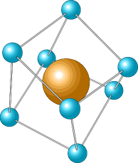
Figure 1: Dodecahedron configuration of O^2- ions around the RE³⁺ impurity ion in the garnet structure. Two different viewing angles are shown.

	YGG			YAG
	x	y	z	x	y	z
O1	1.8690	0.6852	-1.2268	1.8600	0.6076	-1.2152
O2	1.8690	-0.6852	1.2268	1.8600	-0.6076	1.2152
O3	-1.8690	-1.2268	0.6852	-1.8600	-1.2152	0.6076
O4	-1.8690	1.2268	-0.6852	-1.8600	1.2152	-0.6076
O5	0.3082	2.3848	0.3340	0.2858	2.3944	0.3590
O6	-0.3082	0.3340	2.3848	-0.2858	0.3590	2.3944
O7	0.3082	-2.3848	-0.3340	0.2858	-2.3944	-0.3590
O8	-0.3082	-0.3340	-2.3848	-0.2858	-0.3590	-2.3944

Table 2: Coordinates of oxygen ions in YGG and YAG (Å) with respect to the rare earth ion. The axes $x$, $y$, and $z$ are directed along the three orthogonal cube edges $a$, $b$, and $c$, Table 1.

Euler	RE3+ site
angle	1	2	3	4	5	6
$\alpha$	0	$\pi/2$	$\pi$	$3\pi/2$	0	$\pi$
$\beta$	0	0	0	0	$\pi/2$	$\pi/2$
$\gamma$	0	0	0	0	0	0

Table 3: Euler angles of rotation between inequivalent RE³⁺ impurity sites.

III Calculation of the electronic structure of Re$\mathbf{\cdot}$O₈ cluster

We describe an isolated impurity ion with the effective potential in the following parametric form:

$$V_{RE}(r) = \frac{1}{r}\frac{(Z_{i}-Z)(e^{-\frac{\mu}{d}}+1)}{(1+\eta r)^{2}(e^{\frac{r-\mu}{d}}+1)}-\frac{Z_{i}}{r},$$ (5)

Pr $$: \mu=1.0,\ d=1.3,\ \eta=2.25;$$

Tm $$: \mu=1.0,\ d=1.0,\ \eta=2.56.$$

Here $Z$ is the nuclear charge of the impurity ion, $Z_{i}$ is the charge of the electron core of ion, and $\mu$, $d$ and $\eta$ are parameters that describe the core. We use atomic units, expressing energy in units of $E_{0}=27.2\ \textrm{eV}$ and distance in units of the Bohr radius $a_{B}=0.53\times 10^{-8}\ \textrm{cm}$. Solution of the Dirac equation with the potential (5) gives wave functions and energies of the single-electron states. The potential (5) provides a good fit to the experimental energy levels of isolated impurity ions NIST ; the comparison is presented in Table 4.

Ion	Experiment		Calculation
	state	energy	state	energy
Pr2+	4f2(3H4)5d	-155	5d	-153
	4f2(3H4)6s	-146	6s	-146
	4f2(3H4)6p	-114	6p	-114
Pr3+	4f2(3H4)	-314	4f	-313

Ion	Experiment		Calculation
	state	energy	state	energy
Tm2+	4f12(3H6)5d	-163	5d	-163
	4f12(3H6)6s	-165	6s	-167
	4f12(3H6)6p	-126	6p	-126
Tm3+	4f12(3H6)	-344	4f	-345

Table 4: Calculated and experimental NIST energy levels of an isolated ion with respect to the ionization limit. Energy levels are averaged over the fine structure. Units $10^{3}\ \textrm{cm}^{-1}\!$.

In order to model the electronic structure of the RE$\cdot$O₈ cluster (Fig. 1), following MDS we use the jelly model and smear the 8 oxygen ions over a spherical shell around the rare earth ion. Hence, the effective potential due to the oxygen ions at the RE³⁺ site is

$$V_{O}(r)=-A_{o}e^{-\left(\frac{r-r_{o}}{D}\right)^{2}}\!,$$ (6)

where $r_{o}=4.5\ a_{B}$ is the mean RE–O distance, $A_{o}$ and $D$ are parameters of the effective potential. To describe the electrons which contribute to the effect we use the combined spherically symmetric potential

$$V(\boldsymbol{r})=V_{RE}(\boldsymbol{r})+V_{O}(\boldsymbol{r}),$$ (7)

where $V_{RE}$ is the single impurity ion potential (5). Solution of the Dirac equation with potential (7) gives the single-particle orbitals. In this picture we describe the electronic configuration of the cluster as $[\textrm{RE}^{3+}]6s^{2}6p^{6}$, where the electronic configuration of Pr³⁺ is $1s^{2}\!...\,5s^{2}5p^{6}4f^{2}$ and Tm³⁺ is $1s^{2}\!...\,5s^{2}5p^{6}4f^{12}$. The eight states $6s^{2}6p^{6}$ represent $2p_{\sigma}$-electrons of oxygens combined to $S$- and $P$-waves with respect to the central impurity ion (see Ref. MDS ). Parameter $A_{o}$ in the “oxygen” potential $V_{O}$ (6) is determined by matching the wavefunction of oxygen $2p_{\sigma}$-orbital (calculated in Ref. FS ) with the $6s$- and $6p$-orbitals from the combined potential (7) at the radius $R\approx 2.5a_{B}$. The matching conditions are

$$|\psi_{6s}(R)|=|\psi_{2p_{\sigma}}(r_{o}-R,\cos\theta=1)|,$$

$$|\psi_{6p}(R,\cos\theta=1/\sqrt{3})|=|\psi_{2p_{\sigma}}(r_{o}-R,\cos\theta=1)|,$$ (8)

This is a formulation of the idea of dual description at $r\approx R$, see Refs. FS ; Simon .

The parameter $D$ in (6) represents the size of the oxygen core and is about $D\lesssim 1$ (atomic units). The jelly model is rather crude and the value of $D$ cannot be determined precisely, see Ref. MDS . In the present work we vary this parameter in the range of $0.1$–$1.5\,$. For each particular value of $D$ we find $A_{o}$ to satisfy (III), for example $A_{o}=0.9$ at $D=1\,$. The most realistic value for $D$ is probably around $0.5$–$1.0\,$. To be specific, in the final answers we present results at $D=1.0\,$. Instead of the jelly model it would certainly be better to use a relativistic quantum chemistry Hartree-Fock method GQ (or the Kohn-Sham form of the relativistic density functional method which allows one to generate electron orbitals) to describe the RE$\cdot$O₈ cluster. However, this would be a much more involved calculation at the edge of present computational capabilities and therefore, at this stage, we continue with the jelly model.

IV Calculation of the effective Hamiltonian (1)

The calculations in the present section are similar to those performed in MDS for the electric dipole moment of the electron. There are three perturbation operators that contribute to the correlation (1). First, there is a magnetic interaction of the electron with the nuclear anapole moment, see, e.g., Khripl . Expressed in atomic units the interaction reads

$$V_{a} = K_{a}(\boldsymbol{I}\boldsymbol{\alpha})\delta(\boldsymbol{r}),$$ (9)

$$K_{a} = S_{a}\kappa_{a}\left(\frac{Gm^{2}\alpha}{\sqrt{2}}\right)=1.57\cdot 10^{-14}\kappa_{a}S_{a},$$

$$\kappa_{a} = \frac{9}{10}g\frac{\alpha\mu}{m\tilde{r}_{0}}A^{2/3};$$

$${}^{141}\textrm{Pr}:\kappa_{a} = 0.35,\ \ \ \ S_{a}=-0.34,$$

$${}^{169}\textrm{Tm}:\kappa_{a} = 0.39,\ \ \ \ S_{a}=-0.25.$$

Here $m$ is the electron mass, $G$ is the Fermi constant, and $\alpha$ is the fine structure constant; $\boldsymbol{\alpha}$ are the Dirac matrices, $\mu$ is the magnetic moment of the unpaired nucleon (proton in these cases) expressed in nuclear magnetons, $\tilde{r}_{0}=1.2fm$, $A$ is the mass number of the nucleus, and $g\approx 4$ for outer proton and $g\sim 1$ for outer neutron. Values of the nuclear structure constant $S_{a}$ have been calculated in MS .

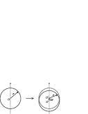
Figure 2: Schematic picture, illustrating the shift of ${V_{O}(\boldsymbol{r})}$ due to the lattice deformation.

The second perturbation operator is related to the shift $\Delta\boldsymbol{r}$ of the rare earth ion with respect to the surrounding oxygen ions. The shift is proportional to the external electric field, but for now we consider $\Delta\boldsymbol{r}$ as an independent variable. In the jelly model $-\Delta\boldsymbol{r}$ is the shift of the spherically symmetric oxygen potential $V_{O}(r)$ (6) with respect to the origin, see Fig. 2. Therefore,

$$V_{O}(\boldsymbol{r})\rightarrow V^{{}^{\prime}}_{O}(\boldsymbol{r}) = V_{O}(\boldsymbol{r}+\Delta\boldsymbol{r})=V_{O}(\boldsymbol{r})+\frac{(\Delta\boldsymbol{r\cdot r)}}{r}\frac{\partial V_{O}}{\partial r}$$ (10)

Thus, the perturbation operator related to the lattice deformation reads

$$V_{1}(\boldsymbol{r}) = \frac{(\Delta\boldsymbol{r\cdot r)}}{r}\frac{\partial V_{O}}{\partial r}=\left(\Delta x\sin\theta\cos\phi+\Delta y\sin\theta\sin\phi+\Delta z\cos\theta\right)(-2)\frac{(r-r_{o})}{D^{2}}V_{O}(r).$$ (11)

Here $\boldsymbol{r}=r(\sin\theta\cos\phi,\sin\theta\sin\phi,\cos\theta)$.

The third perturbation is the residual electron-electron Coulomb interaction, which is not included in the effective potential,

$$V_{C}(\boldsymbol{r}_{i},\boldsymbol{r}_{j})=\frac{1}{|\boldsymbol{r}_{i}-\boldsymbol{r}_{j}|}=\sum_{lm}\frac{4\pi}{2l+1}\frac{r_{<}^{l}}{r_{>}^{l+1}}Y^{*}_{lm}(\boldsymbol{r}_{i})Y_{lm}(\boldsymbol{r}_{j}).$$ (12)

Here $\boldsymbol{r}_{i}$ and $\boldsymbol{r}_{j}$ are radius-vectors of the two interacting electrons.

The formula for the energy correction in the third order of perturbation theory reads, see, e.g., Ref. LL :

$$E_{n}^{(3)}=\sum_{m}{}^{{}^{\prime}}\sum_{k}{}^{{}^{\prime}}\frac{V_{nm}V_{mk}V_{kn}}{\hbar^{2}\omega_{mn}\omega_{kn}}-V_{nn}\sum_{m}{}^{{}^{\prime}}\frac{|V_{nm}|^{2}}{\hbar^{2}\omega_{nm}^{2}},$$ (13)

where $V=V_{a}+V_{1}+V_{C}$. In Eq. (13) we need to consider only the terms that contain all the operators $V_{a}$, $V_{1}$, and $V_{C}$.

The shift operator $V_{1}$ is nearly saturated by $6s$- and $6p$-states because core electrons do not “see” the deformation of the lattice, hence, for this operator we consider only $s$-$p$ mixing. Matrix elements of the anapole operator $V_{a}$ practically vanish for the electron states with high angular momentum, since this operator is proportional to the Dirac delta function. Therefore, it is sufficient to take into account only $\langle ns_{1/2}|V_{1}|kp_{1/2}\rangle$ matrix elements. All in all, there are 11 diagrams (Fig. 3) that correspond to Eq. (13). All diagrams are exchange ones and contribute with the sign shown before each of the diagrams. Summation over all intermediate states $|k\rangle$ and $|m\rangle$ and over all filled states $|n\rangle$ is assumed.

$-\quad 2\times$		$-\quad 2\times$
	1)		2)
$-\quad 2\times$		$-\quad 2\times$
	3)		4)

$+$		$\times\quad\!\!\Bigg{(}$		$\quad\!\!\!+$		$\Bigg{)}$
		5)

$-\quad 2\times$		$-\quad 2\times$		$-\quad 2\times$
	6)		7)		8)
$-\quad 2\times$		$-\quad 2\times$
	9)		10)

$+$		$\times\quad\!\!\Bigg{(}$		$\quad\!\!\!+$		$\Bigg{)}$
		11)

Figure 3: Third order perturbation theory diagrams corresponding to Eq. (13). The cross denotes the anapole interaction ${V_{a}}$ (9), the dashed line denotes the lattice deformation perturbation ${V_{1}}$ (11), and the wavy line denotes the Coulomb interaction ${V_{C}}$ (12). The multipolarity of the Coulomb interaction is shown near the wavy line. Each diagram contributes with the coefficient shown before the diagram (number of diagrams of this kind). Summation over all intermediate states ${|k\rangle}$ and ${|m\rangle}$ and over all filled states ${|n\rangle}$ is assumed.

Since $V_{a}$ and $V_{1}$ are single-particle operators, we evaluate each diagram by solving equations for the corresponding wavefunction corrections. For example, the first diagram contains in the top right leg the correction

$$|\delta\psi_{x}\rangle=\sum_{m}\frac{\langle mp_{1/2}|V_{1}|ns\rangle}{\epsilon_{ns}-\epsilon_{mp_{1/2}}}|mp_{1/2}\rangle.$$ (14)

To evaluate the correction we do not use a direct summation, but instead solve the equation

$$(H-\epsilon)|\delta\psi_{x}\rangle=-V_{1}|ns\rangle,\ \ \ \epsilon=\epsilon_{ns}$$ (15)

for each particular $|ns\rangle$ state. Here $H$ is the Dirac Hamiltonian with the potential (7). Similarly, the bottom left leg of the same diagram is evaluated using

$$(H-\epsilon_{ns})\delta\psi_{d}=-V_{a}|ns\rangle.$$ (16)

In solving this equation we take the finite size of the nucleus into account by replacing the $\delta$-function in (9) with a realistic nuclear density.

Apart from the coefficients presented in Fig. 3, which in essence show the number of diagrams of each kind, each particular diagram in Fig. 3 contributes with its own angular coefficient. In calculating the coefficients we assumed, without loss of generality, that the total angular momentum of the $4f$-electrons is directed along the $z$-axis, $|J,J_{z}\rangle$. Values of the coefficients are presented in Table 8 in the Appendix. The method for separating the radial equations corresponding to (15) and (16) is also described in the Appendix. As the result of the calculations we find the following $P$-odd energy correction related to the displacement $\Delta\boldsymbol{r}$ of the RE impurity ion:

$$\Delta\epsilon=K_{a}\alpha A\frac{1}{a_{B}}(\boldsymbol{\Delta r}\cdot[\boldsymbol{I}\times\boldsymbol{J}])E_{0}.$$ (17)

We recall that $\boldsymbol{I}$ is spin of the nucleus, $\boldsymbol{J}$ is the total angular momentum of the $f$-electrons, $E_{0}=27.2\ \textrm{eV}$ is the atomic unit of energy, $a_{B}$ is the Bohr radius, $\alpha$ is the fine structure constant, and $K_{a}$ is given in Eq. (9). The dimensionless coefficient $A$ for the Pr³⁺ and Tm³⁺ ions (in the corresponding lattices) calculated at $D=1.0$ in Eq. (6) reads:

$$A_{\mathrm{Pr}} = -25.99-11.20+0.32+0.59+18.64-18.99$$

$${}+0.58+1.39-15.99+28.37+25.73=3.45,$$

$$A_{\mathrm{Tm}} = 9.77+12.78-3.58-1.33-32.24+36.49$$ (18)

$${}+0.21+0.12+53.48-67.70-10.95=-2.95.$$

The eleven terms in (18) represent the contributions of the eleven diagrams in Fig. 3. As one can see, there is significant compensation between different terms in (18). This compensation is partially related to the fact that each particular diagram in Fig. 3 contains contributions forbidden by the Pauli principle. These contributions are canceled out only in the sum of the diagrams. To check (18) we have also performed a more involved calculation explicitly taking into account the Pauli principle in each particular diagram, the results read:

$$A_{\mathrm{Pr}} = -0.07-0.18+1.48+0.72+1.00-2.63$$

$${}-1.74+0.88+41.34-40.00+2.65=3.45,$$

$$A_{\mathrm{Tm}} = -0.55-0.56-4.09-1.36-1.47+6.27$$ (19)

$${}+0.53+0.15-38.94+38.06-0.99=-2.95.$$

Although each individual term has changed compared to (18), the total sum of the diagrams remains the same. Comparison between (18) and (19) is a test of the many body perturbation theory used in the calculation. To demonstrate the sensitivity to parameters of the effective potential, we plot in Fig. 4 the coefficient $A$ versus the width $D$ of the oxygen potential, see Eq. (6). As we pointed out in Section III, the most realistic value of $D$ is around $0.5$–$1.0\,$. To be specific, in the final estimates we use the results (18) and (19), which correspond to the value $D=1.0\,$.

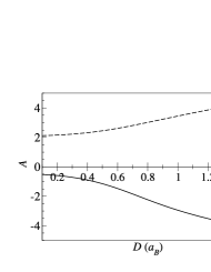
Figure 4: Value of the coefficient $A$ defined in Eq. (17) versus width of the effective oxygen potential. The dashed line corresponds to Pr³⁺ in YGG and the solid line corresponds to Tm³⁺ ions in YAG.

V Calculation of the effective Hamiltonian (3)

The $P$-odd effective Hamiltonian considered in the previous section arises due to a shift of the environment with respect to the rare earth ion. In other words, it is due to the first harmonic in the electron density induced by the perturbation operator $V_{1}$ (11). In the equilibrium position the first harmonic vanishes identically due to the symmetry of the lattice. The next harmonic in the electron density that contributes to the parity nonconserving effect is the third harmonic which is nonzero even in the equilibrium position of the rare earth ion. This effect gives the $P$-odd energy shift even in the absence of an external electric field.

The effective oxygen potential $V_{O}$ (6) represents the spherically symmetric part of the real potential for electrons created by the eight oxygen ions in the garnet lattice. Let us describe the potential (pseudopotential) of a single oxygen ion as $g\delta(\boldsymbol{r}-\boldsymbol{R})$, where $\boldsymbol{R}$ is the position of the ion and $g$ is some constant. Then the total potential is

$$V(\boldsymbol{r})=\sum_{\boldsymbol{R}}g\delta(\boldsymbol{r}-\boldsymbol{R}),$$ (20)

where summation is performed over the coordinates of the eight oxygen ions presented in Table 2. Expanding the Dirac delta function in the potential $V(\boldsymbol{r})$ in a series of spherical harmonics, we find

$$V(\boldsymbol{r})=g\frac{\delta(r-R)}{R^{2}}\sum_{km}\sum_{\boldsymbol{R}}Y^{*}_{km}(\boldsymbol{R})\cdot Y_{km}(\boldsymbol{r}).$$ (21)

Then,

$$V_{O}(\boldsymbol{r}) = g\frac{\delta(r-R)}{R^{2}}\sum_{\boldsymbol{R}}Y_{00}(\boldsymbol{R})\cdot Y_{00}(\boldsymbol{r})\to-A_{o}e^{-\left(\frac{r-r_{o}}{D}\right)^{2}}\!,$$ (22)

and hence the third harmonic reads

$$V_{3}(\boldsymbol{r}) = g\frac{\delta(r-R)}{R^{2}}\sum_{\boldsymbol{R}}Y^{*}_{3m}(\boldsymbol{R})\cdot Y_{3m}(\boldsymbol{r})\to-A_{o}e^{-\left(\frac{r-r_{o}}{D}\right)^{2}}\frac{\pi}{2}T_{3m}\cdot Y_{3m}(\boldsymbol{r}),$$ (23)

$$T_{3m} = \sum_{\boldsymbol{R}}Y^{*}_{3m}(\boldsymbol{R}).$$

The spherical tensor $T_{3m}$ (lattice octupole) for yttrium aluminium garnet and yttrium gallium garnet has only one non-zero independent component, $T_{31}=-0.1876$ for YAG and $T_{31}=-0.1010$ for YGG. All other components are determined by the following relations:

$$T_{33}=\sqrt{\frac{3}{5}}T_{31},\ \ T_{3\,\textrm{-}1}=-T_{31},\ \ T_{3\,\textrm{-}3}=-T_{33},\ \ T_{30}=0.$$ (24)

Components of the corresponding Cartesian irreducible tensor $T_{klm}$ can be found using the following relations:

$$T_{xzz}=T_{zxz}=T_{zzx}=-T_{xyy}=-T_{yxy}=-T_{yyx}=-\sqrt{\frac{8}{15}}T_{31}.$$ (25)

All other components of the Cartesian tensor are equal to zero.

Similar to the “dipole” effect considered in the previous section, the octupole effect arises in the third order of perturbation theory. The relevant perturbation theory operators are a) interaction of the electron with the nuclear anapole moment $V_{a}$ (9), b) interaction of the electron with the lattice octupole harmonic $V_{3}$ (23), and c) the residual electron-electron Coulomb interaction $V_{C}$ (12). The formula for the energy correction (13) yields 7 diagrams which are presented in Fig. 5.

$-\quad 2\times$		$-\quad 2\times$
	1)		2)
$-\quad 2\times$
	3)
$-\quad 2\times$		$-\quad 2\times$
	4)		5)
$-\quad 2\times$		$-\quad 2\times$
	6)		7)

Figure 5: Diagrams for the “octupole” effect. The cross denotes the anapole interaction ${V_{a}}$ (9), the dashed line denotes the lattice octupole ${V_{3}}$ (V), and the wavy line denotes the Coulomb interaction ${V_{C}}$ (12). The multipolarity of the Coulomb interaction is shown near the wavy line. Each diagram contributes with the coefficient shown before the diagram (number of diagrams of this kind). Summation over all intermediate states ${|k\rangle}$ and ${|m\rangle}$ and over all filled states ${|n\rangle}$ is assumed.

Besides the coefficients presented in Fig. 5, which show the number of diagrams of each kind, each particular diagram in Fig. 5 contributes with its own angular coefficient. In calculating the coefficients we assumed, without loss of generality, that the total angular momentum of $4f$ electrons is directed along the $z$-axis, $|J,J_{z}\rangle$, and the nuclear spin is directed along the $y$-axis, $\boldsymbol{I}=(0,I,0)$. The angular coefficients for each of the 7 diagrams from Fig. 5 are presented in Table 8 in the Appendix. The method for separating the radial equations is also described in the Appendix. The effective Hamiltonian for the lattice octupole effect has the following form

$$\Delta\epsilon=K_{a}\alpha BI_{i}\epsilon_{ijk}T_{klm}\left(J_{j}J_{l}J_{m}+J_{m}J_{l}J_{j}\right)E_{0}.$$ (26)

Eq. (26) represents the only $P$-odd scalar combination one can construct from the two vectors and one irreducible third rank tensor. Note, that $\boldsymbol{J}$ here is an operator, and different components of $\boldsymbol{J}$ do not commute. This is why in the right hand side of Eq. (26) we explicitly write the Hermitian combination. The matrix element of (26) in the kinematics which we consider for the calculation of the angular coefficients (Table 8) is

$$\langle J,J_{z}|I_{i}\epsilon_{ijk}T_{klm}\left(J_{j}J_{l}J_{m}+J_{m}J_{l}J_{j}\right)|J,J_{z}\rangle=T_{zzx}IJ_{z}[5J_{z}^{2}-3J(J+1)+1].$$ (27)

Our calculations show that contributions of the diagrams with the intermediate $f$-state (diagrams 4,5,6,7 in Fig. 5) are at least 30 times smaller compared to diagrams 1 and 2. The reason for this is very simple: $f$-electrons are practically decoupled from the lattice deformation. The diagram 3 is even smaller because internal $3d$- and $4d$-electrons are also decoupled from the lattice. So, only diagrams 1 and 2 contribute to the effect and they are nearly saturated by the intermediate unoccupied $5d$-state. The dimensionless coefficient $B$ for Pr and Tm ions in corresponding lattices calculated at $D=1.0$ [Eq. (6)] reads:

$$B_{\mathrm{Pr}}(D=1) = -2.18+0.76=-1.42,$$

$$B_{\mathrm{Tm}}(D=1) = 1.11-0.45=0.66.$$ (28)

The two terms in equations (28) represent the contributions of the first and second diagrams. The variation of the coefficient $B$ with the width of the effective oxygen potential $D$ is shown in Fig. 6. Again, we recall that the most realistic value of $D$ is around $0.5$–$1.0\,$. To be specific, in the estimates for the effect we use $D=1.0\,$.

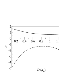
Figure 6: Value of the coefficient $B$ in Eq. (26) versus the width of the effective oxygen potential. Dashed line corresponds to Pr³⁺ in YGG and solid line corresponds to Tm³⁺ in YAG.

VI Crystal field, average electron magnetization, orientation of nuclear spin

The energy of a free ion is degenerate with respect to the $z$-projection of total angular momentum. Interaction with the lattice (crystal field) breaks the rotational invariance and lifts the degeneracy. The effective crystal-field Hamiltonian can be written in the following form, see, e.g., CFI

$$H_{\textrm{\it cf}}=\sum_{km}B^{*}_{km}\sum_{i}\sqrt{\frac{4\pi}{2k+1}}Y_{km}(\boldsymbol{r})$$ (29)

where $B_{km}$ are the crystal field parameters, $\boldsymbol{r}$ is the radius-vector of the atomic electron.

Experimental values of the energy levels for Pr³⁺ in YGG and Tm³⁺ in YAG are known Pr ; Tm , and fits of the crystal field parameters $B_{km}$ have been performed in the experimental papers. Unfortunately, we cannot use these fits because they are performed without connection to a particular orientation of crystallographic axes. We need to know the connection and therefore we have performed independent fits. For the fits we use a modified point-charge model. In the simple point-charge model the crystal field is of the form

$$A_{km}^{(pc)} = -\sum_{j}\frac{q_{j}}{r_{j}^{k+1}}\sqrt{\frac{4\pi}{2k+1}}Y_{km}(\boldsymbol{r}_{j}),$$ (30)

$$B_{km}^{(pc)} = \rho_{k}A_{km}^{(pc)},$$ (31)

where $j$ enumerates ions of the lattice and $\rho_{k}=\langle r^{k}\rangle$ is the expectation value over the RE $f$-electron wave function. The values of $\rho_{k}$ are known CFI . The point charges are $q_{O}=-2$ and $q_{Y}=q_{\textrm{\it Ga}}=q_{\textrm{\it Al}}=3$. Clearly, the naive point-charge model is insufficient to describe the nearest 8 oxygen ions because of the relatively large size of the ions (extended electron density of the host oxygens). To describe the effect of the extended electron density we introduce an additional field $A_{km}^{(el)}$

$$A_{km} = A_{km}^{(pc)}+A_{km}^{(el)},$$ (32)

$$A_{km}^{(el)} = -\alpha_{k}\sum_{j=1}^{8}\frac{q_{j}}{r_{j}^{n+1}}\sqrt{\frac{4\pi}{2n+1}}Y_{km}(\boldsymbol{r}_{j}),$$ (33)

here the sum runs over the eight oxygen ions surrounding the dopant ion in the garnet structure, and $\alpha_{k}$ are fitting parameters. So, we have only three fitting parameters, $\alpha_{2}$, $\alpha_{4}$, and $\alpha_{6}$, because higher multipoles do not contribute in $f$-electron splitting. In the end, we get a fairly good fit of the experimental energy levels, see Table 5. The values of the resulting crystal field parameters $B_{km}$ are presented in Table 6.

Pr3+:YGG		Tm3+:YAG
Exp. Pr	Calc.	Exp. Tm	Calc.
0	0	0	0
23	23	27	27
23	23	216	182
-	400	240	240
532	413	247	253
578	538	300	301
598	621	450	306
626	877	588	494
689	895	610	609
		650	673
		690	686
		730	825
		-	937

Table 5: Experimental and calculated crystal field energy levels in $cm^{-1}$. $J$-$J$ mixing is neglected in the calculation.

Compound	$B_{20}$	$B_{21}$	$B_{22}$	$B_{40}$	$B_{41}$	$B_{42}$	$B_{43}$	$B_{44}$	$B_{60}$	$B_{61}$	$B_{62}$	$B_{63}$	$B_{64}$	$B_{65}$	$B_{66}$
Pr:YGG	622	11$i$	-762	211	-475$i$	727	1256$i$	-423	963	-280$i$	-648	-437$i$	91	304$i$	-961
Tm:YAG	257	92$i$	-315	-1198	344$i$	-248	-909$i$	-523	-938	528$i$	569	816$i$	94	-563$i$	843

Table 6: Crystal field parameters in cm^-1, that fit the energy levels in Table 5.

For the non-Kramers ions, such as Pr³⁺ and Tm³⁺, the expectation value of the total angular momentum in the ground state vanishes due to the crystal field, $\langle\boldsymbol{J}\rangle=0$. To get a nonzero $\langle\boldsymbol{J}\rangle$ one needs to apply an external magnetic field $\boldsymbol{B}$. Diagonalizing the Hamiltonian matrix of the dopant ion in the magnetic field

$$\langle J^{\prime}_{z}|H_{\textrm{\it cf}}+\mu_{B}g(\boldsymbol{J}\boldsymbol{B})|J_{z}\rangle,$$ (34)

($9\times 9$ matrix for Pr³⁺ and $13\times 13$ matrix for Tm³⁺) we find the ground state of the ion in the presence of the external magnetic field $B$ (here $\mu_{B}$ is the Bohr magneton and $g$ is the atomic Lande factor; $g=0.80$ for Pr³⁺ in ${}^{3}\!H_{4}$ configuration and $g=1.17$ for Tm³⁺ in ${}^{3}\!H_{6}$ configuration.) For weak magnetic field the average total angular momentum can be written as

$$\langle J_{i}\rangle=\tau_{ik}B_{k}.$$ (35)

The tensor $\tau_{ik}$ can be diagonalized. According to our calculations, both for Pr and Tm it is diagonal with the principal axes $\boldsymbol{n}_{1}=(1,0,0)$, $\boldsymbol{n}_{2}=(1,1/\sqrt{2},1/\sqrt{2})$, $\boldsymbol{n}_{3}=(1,1/\sqrt{2},-1/\sqrt{2})$:

$$\textrm{Pr}:\ \ \ \ \tau=\left(\begin{array}[]{ccc}-0.003&0&0\\ 0&-0.154&0\\ 0&0&-0.176\end{array}\right)\frac{1}{tesla},\ \ \ \ \ \ \textrm{Tm}:\ \ \ \ \tau=\left(\begin{array}[]{ccc}-0.474&0&0\\ 0&-0.023&0\\ 0&0&-0.032\end{array}\right)\frac{1}{tesla}.$$ (42)

The average total electron angular momentum in the magnetic fields applied along the directions $\boldsymbol{n}_{1}$, $\boldsymbol{n}_{2}$, and $\boldsymbol{n}_{3}$ is plotted in Fig. 7. We see that the linear expansion (35) is valid for the field $B<5$–10 T.

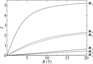
Figure 7: The average total electron angular momentum of the rare earth ion versus magnetic field (tesla). Directions of the magnetic field correspond to the principal axes of the magnetization tensor $\boldsymbol{n}_{1}$, $\boldsymbol{n}_{2}$, and $\boldsymbol{n}_{3}$. Solid lines correspond to Tm³⁺ in YAG and dashed lines correspond to Pr³⁺ in YGG.

The effective Hamiltonian for the nuclear spin is

$$H_{\textrm{\it nuc}}=A_{\textrm{\it hf}}(\boldsymbol{J\cdot I})-\frac{\mu\mu_{N}}{I}(\boldsymbol{B\cdot I}),$$ (43)

where $A_{\textrm{\it hf}}$ is the hyperfine constant, $\mu$ is the nuclear magnetic moment in nuclear magnetons and $\mu_{N}$ is the nuclear magneton:

$${}^{141}\textrm{Pr} : \ A_{\textrm{\it hf}}=1093\ \textrm{MHz}\ \textrm{\cite[cite]{\@@bibref{Authors Phrase1YearPhrase2}{ahf}{\@@citephrase{(}}{\@@citephrase{)}}}},\ \mu=4.2754\ \textrm{\cite[cite]{\@@bibref{Authors Phrase1YearPhrase2}{tabisot}{\@@citephrase{(}}{\@@citephrase{)}}}},\ I=5/2;$$

$${}^{169}\textrm{Tm} : \ A_{\textrm{\it hf}}=-393.5\ \textrm{MHz}\ \textrm{\cite[cite]{\@@bibref{Authors Phrase1YearPhrase2}{ahf}{\@@citephrase{(}}{\@@citephrase{)}}}},\ \mu=-0.2316\ \textrm{\cite[cite]{\@@bibref{Authors Phrase1YearPhrase2}{tabisot}{\@@citephrase{(}}{\@@citephrase{)}}}},\ I=1/2.$$ (44)

Pr	Tm

Figure 8: The NMR frequency versus the orientation of magnetic field with respect to the crystallographic axes, $B=10\ \textrm{T}$. We show the dependence on $\phi$ for different values of $\theta$.

Equation (43), together with (35), gives the NMR frequency $\nu$. Dependence of the frequency on the orientation of the magnetic field $\boldsymbol{B}=B(\sin\theta\cos\phi,\sin\theta\sin\phi,\cos\theta)$ with respect to the crystallographic axes is plotted in Fig. 8, we take $B=10T$. Equation (43) also defines the quantization axis for the nuclear spin:

$$\boldsymbol{n}_{I}\propto\left(A_{\textrm{\it hf}}\langle\boldsymbol{J}\rangle-\frac{\mu\mu_{N}}{I}\boldsymbol{B}\right)=\left(A_{\textrm{\it hf}}\hat{\tau}\boldsymbol{B}-\frac{\mu\mu_{N}}{I}\boldsymbol{B}\right).$$ (45)

This allows us to find cross product $\boldsymbol{n}_{I}\times\boldsymbol{J}$ that appears in the anapole induced energy correction (1), (17):

$$M=|\boldsymbol{n}_{I}\times\boldsymbol{J}|=\frac{|\mu\mu_{N}[\boldsymbol{B}\times(\hat{\tau}\boldsymbol{B})]|}{|IA_{\textrm{\it hf}}(\hat{\tau}\boldsymbol{B})-\mu\mu_{N}\boldsymbol{B}|}.$$ (46)

The value of $M$ depends on the magnitude and the orientation of the external magnetic field $\boldsymbol{B}$ with respect to the crystallographic axes. At $B=10\ \textrm{T}$ the maximum value of $M$ is

Pr $$: M=1.02\cdot 10^{-1},$$

Tm $$: M=0.79\cdot 10^{-1}.$$ (47)

Unfortunately, the values of $M$ are relatively small compared to the maximum possible value $M=J$ (4 for Pr and 6 for Tm). The suppression is due to the fact that in the nuclear magnetic Hamiltonian (43) the hyperfine interaction $A_{\textrm{\it hf}}(\boldsymbol{J\cdot I})$ is an order of magnitude larger than the direct magnetic interaction $\mu\mu_{N}(\boldsymbol{B\cdot I})/I$, while to maximize $M$ one has to have these interactions comparable. In spite of the suppression, the observable effects related to the effective Hamiltonian (1), (17) are quite reasonable (see next Section).

The situation with the effective interaction (3), (26) is different. Looking at equations (3), (26) one can expect at first sight that the corresponding energy shift is nonzero only if $\boldsymbol{I}\times\langle\boldsymbol{J}\rangle\neq 0$. However, this is incorrect. The point is that due to the crystal field the tensor $\langle J_{j}J_{l}J_{m}+J_{m}J_{l}J_{j}\rangle$ has nonzero components orthogonal to $\langle\boldsymbol{J}\rangle$. And the octupole induced energy shift is in fact maximum when $\boldsymbol{I}\ \|\ \langle\boldsymbol{J}\rangle$. The dependence of the kinematic coefficient (see Eq. (26))

$$N=\frac{1}{I}I_{i}\epsilon_{ijk}T_{klm}\langle J_{j}J_{l}J_{m}+J_{m}J_{l}J_{j}\rangle$$ (48)

on the orientation of magnetic field $\boldsymbol{B}=B(\sin\theta\cos\phi,\sin\theta\sin\phi,\cos\theta)$ at $B=10\ \textrm{T}$ is plotted in Fig. 9. The maximum value of $N$ is

Pr $$: \ \ \ N=1.81,$$

Tm $$: \ \ \ N=2.42.$$ (49)

Pr	Tm

Figure 9: The kinematic coefficient $N$ (48) in the lattice octupole induced energy correction versus orientation of magnetic field with respect to the crystallographic axes, $B=10\ \textrm{T}$. We show the dependence on $\phi$ for different values of $\theta$.

The calculations in the present section are based on the fit of experimental energy levels, Table 5, using the crystal field parameters. We use the set of parameters presented in Table 6. Unfortunately, the set is not unique and there are other sets which also reasonably fit the energy levels. In particular, for Tm³⁺ in YAG there is a set of parameters which gives a lattice octupole induced PNC energy shift an order of magnitude larger than the present set. At this stage we prefer to continue with the conservative estimate. To elucidate the uncertainty related to the crystal field parameters detailed measurements of NMR frequencies, as well as transition amplitudes, are necessary.

VII Estimates of observable effects

The effect (1), (17) requires a displacement of the impurity ion from its equilibrium position. Such displacement can be achieved by application of an external electric field. The displacement has been estimated in Ref. MDS in relation to the discussion of electric dipole moments. The idea behind the estimate is very simple. Since the Ga–O link in YGG and the Al–O link in YAG are much more rigid than the Y–O links (see discussion in MDS ) the electrostatic polarization in YGG and YAG is mainly due to displacement of the yttrium ions

$$\boldsymbol{P}=3en\Delta\boldsymbol{r}.$$ (50)

On the other hand, the dielectric polarization caused by the external electric field $\boldsymbol{E}$ is

$$\boldsymbol{P}=\frac{\epsilon-1}{4\pi}\boldsymbol{E},$$ (51)

where the static dielectric constant is $\epsilon\approx 12$ for YGG and YAG. This yields the following expression for the displacement of the yttrium ions:

$$\Delta\boldsymbol{r} = \frac{\epsilon-1}{4\pi}\frac{\boldsymbol{E}}{3en},$$

$$\Delta{r}/a_{B} = 3.0\cdot 10^{-8}E[\frac{\textrm{V}}{\textrm{cm}}].$$ (52)

Measurements of infrared spectra, as well as measurements of the dependence of the dielectric constant on the concentration of impurities, can help to improve the estimate (VII).

Using (17), together with (47) and (VII), we obtain the following estimates for the NMR frequency shift ($\Delta I=1$) due to the nuclear anapole moment:

Pr $$: \Delta\nu\sim 0.9\times 10^{-9}E[\frac{\textrm{V}}{\textrm{cm}}]\ \textrm{Hz},$$

Tm $$: \Delta\nu\sim 0.5\times 10^{-9}E[\frac{\textrm{V}}{\textrm{cm}}]\ \textrm{Hz}.$$ (53)

An alternative possibility for the experiment is to provide the maximum possible value of the cross product $\boldsymbol{I}\times\boldsymbol{J}$ by applying an RF pulse and then to measure the induced electric field. Using (17), together with estimates of the elastic constant with respect to the shift of the rare earth ion performed in MDS , we arrive at the following values of the anapole induced electric field:

Pr $$: E\sim 1.4\times 10^{-6}\ \textrm{V/cm},$$

Tm $$: E\sim 0.4\times 10^{-6}\ \textrm{V/cm}.$$ (54)

The field precesses around the direction of the magnetic field with a frequency of about 1 GHz due to the nuclear spin precession. In the estimates (VII) we assume that all yttrium ions are substituted by the rare earth ions.

Another manifestation of nuclear anapole moment is the static perpendicular macroscopic magnetization induced by an external electric field,

$$\delta\boldsymbol{I}\propto\boldsymbol{B}\times\boldsymbol{E}.$$ (55)

The exact value of the macroscopic magnetization depends on temperature and other experimental conditions, therefore we cannot present a specific value. However, we can compare the effect with that expected in the electron EDM experiment Lam (correlation $\delta\boldsymbol{J}\propto\boldsymbol{E}$) using the present experimental limit on $d_{e}$ Com , $d_{e}=1.6\times 10^{-27}e\ \textrm{cm}$, as a reference point. The effective anapole interaction (17) is four order of magnitude larger than the similar effective EDM interaction MDS . On the other hand, the electron EDM interaction causes electron magnetization whereas the anapole interaction causes only nuclear magnetization, so we lose 3 orders of magnitude on the value of the magnetic moment. Therefore, altogether, one should expect that the anapole magnetization is several times larger than the EDM magnetization.

The effective interaction (26) is independent of the external electric field and is due to the asymmetric environment of the rare earth ion site. Since there is always another site within the unit cell which is the exact mirror reflection of the first one, the energy correction (26) does actually lead to the NMR line splitting. Using Eqs. (26), (28), (48), and (VI), we find the maximum value of this splitting corresponding to the magnetic field $B=10\ \textrm{T}$:

Pr $$: \Delta\nu\sim 0.5\ \textrm{Hz},$$

Tm $$: \Delta\nu\sim 0.25\ \textrm{Hz}.$$ (56)

The splitting depends on the orientation of the magnetic field with respect to the crystallographic axes, see Fig. 8.

VIII Conclusions

In the present work we have considered effects caused by the nuclear anapole moment in thulium doped yttrium aluminium garnet and praseodymium doped yttrium gallium garnet. There are two effects related to the frequency of NMR: 1) NMR line shift in combined electric and magnetic fields. The shift is about $10^{-5}$ Hz at $B=10$ T and $E=10$ kV/cm. 2) NMR line splitting (magnetic field only). The spitting is about 0.5 Hz at $B=10$ T. The value of the splitting depends on the orientation of the magnetic field with respect to the crystallographic axes. Another PNC effect is the induced RF electric field orthogonal to the plane of the magnetic field and nuclear spin, $\boldsymbol{E}\propto[\boldsymbol{B}\times\boldsymbol{I}]$. The field is $E\sim 10^{-6}\ \textrm{V/cm}$ at magnetic field $B=5$–10 T. The last effect we have discussed is unrelated to NMR. This is a variation of the static macroscopic magnetization in combined electric and magnetic fields, $\delta\boldsymbol{M}\propto\boldsymbol{B}\times\boldsymbol{E}$. The magnitude of the effect is several times larger than that expected in the electric dipole moment experiment Lam .

It is our pleasure to acknowledge very helpful discussions with D. Budker, V.V. Yashchuk, A.O. Sushkov and A.I. Milstein.

IX Appendix. Radial equations

In order to calculate the energies and wavefunctions of unperturbed states of the single impurity ion in the garnet environment, we use the Dirac equation

$$(H-\epsilon)|\psi\rangle=0.$$ (57)

The effective potential $V(r)$ (7) in the Dirac Hamiltonian $H$ is spherically symmetric, and thus the two-component wavefunction $|\psi\rangle$ is of the form

$$|\psi\rangle=\frac{1}{r}{f(r)\Omega_{\kappa}\choose i\alpha g(r)\widetilde{\Omega}_{\kappa}}.$$ (58)

Here $\Omega_{\kappa}$ and $\widetilde{\Omega}_{\kappa}$ are the spherical spinors and $f(r)$ and $g(r)$ are radial wavefunctions. Substituting expression (58) for $|\psi\rangle$ into the Dirac equation (57), one gets the following radial equations

$$f^{\prime}+\kappa f/x+(-2+\alpha^{2}(V-\epsilon))g=0,$$

$$g^{\prime}-\kappa g/x-(V-\epsilon)f=0.$$ (59)

Here $x=r/a_{B}$ is the radius in atomic units; $\kappa=(-1)^{j+1/2-l}(j+1/2)$, where $j$ and $l$ are the total and orbital angular momenta of the single-electron state correspondingly; the potential $V(x)$ ,as well as the energy $\epsilon$, is expressed in atomic energy units. Solving the system of equations (59) as an eigenvalue problem numerically on a logarithmic coordinate grid, we find energies and wavefunctions of the unperturbed states.

The inhomogeneous Dirac equations (15) and (16) are of the form

$$(H-E)|\delta\psi\rangle=-\hat{V}_{p}|\psi\rangle,$$ (60)

where $\hat{V}_{p}$ is the single-particle perturbation operator. The correction $|\delta\psi\rangle$ is of the form

$$|\psi\rangle=\frac{1}{r}{F(r)\Omega_{\kappa^{\prime}}\choose i\alpha G(r)\widetilde{\Omega}_{\kappa^{\prime}}},$$ (61)

and hence the corresponding radial equations are

$$F^{\prime}+\kappa^{\prime}F/x+(-2+\alpha^{2}(V-\epsilon))G=R_{f}\langle\Omega_{\kappa^{\prime}}|\hat{\Phi}|\Omega_{\kappa}\rangle,$$

$$G^{\prime}-\kappa^{\prime}G/x-(V-\epsilon)F=R_{g}\langle\tilde{\Omega}_{\kappa^{\prime}}|\hat{\Phi}|\tilde{\Omega}_{\kappa}\rangle.$$ (62)

The operator $\hat{\Phi}$ represents the angular part of the perturbation $\hat{V}_{p}$, and $R_{f}$ and $R_{g}$ are the radial parts of the perturbation. The functions $R_{f}$, $R_{g}$, and $\hat{\Phi}$ for all the cases we need in the present work are presented in Table 7.

	$\hat{V}_{p}=V_{a},(\ref{pert1})$	$\hat{V}_{p}=V_{a},(\ref{pert1})$	$\hat{V}_{p}=V_{1},(\ref{pert2})$	$\hat{V}_{p}=V_{3},(\ref{pert3m})$
	$|\psi\rangle=|ns_{1/2}\rangle$	$|\psi\rangle=|np_{1/2}\rangle$	$|\psi\rangle=|ns_{1/2}\rangle$ or $|\psi\rangle=|np_{1/2}\rangle$	$|\psi\rangle=|ns_{1/2}\rangle$ or $|\psi\rangle=|np_{1/2}\rangle$
$R_{f}$	$-K_{a}\alpha\rho_{n}(x)f(x)$	$-\frac{1}{3}K_{a}\alpha\rho_{n}(x)f(x)$	$-2\frac{(r-r_{o})}{D^{2}}A_{o}e^{-\left(\frac{r-r_{o}}{D}\right)^{2}}\alpha^{2}g(x)$	$A_{o}e^{-\left(\frac{r-r_{o}}{D}\right)^{2}}\alpha^{2}g(x)$
$R_{g}$	$\frac{1}{3}K_{a}\alpha\rho_{n}(x)g(x)$	$K_{a}\alpha\rho_{n}(x)g(x)$	$2\frac{(r-r_{o})}{D^{2}}A_{o}e^{-\left(\frac{r-r_{o}}{D}\right)^{2}}f(x)$	$-A_{o}e^{-\left(\frac{r-r_{o}}{D}\right)^{2}}f(x)$
$\hat{\Phi}$	$-2i(\boldsymbol{I\cdot j})$	$2i(\boldsymbol{I\cdot j})$	$\Delta x\sin\theta\cos\phi+\Delta y\sin\theta\sin\phi+\Delta z\cos\theta$	$\frac{\pi}{2}T_{3m}\cdot Y_{3m}(\boldsymbol{r})$

Table 7: The functions $R_{f}$, $R_{g}$ and $\hat{\Phi}$ for the different perturbation operators and different states $|\psi\rangle$. $\rho_{n}$ is nuclear density normalized to unity.

Diagram	Pr3+	Tm3+
Dipole effect
1,7,8,11	$\frac{2^{2}\cdot 43}{3^{2}\cdot 5^{3}\cdot 7}F(2)-\frac{2\cdot 19}{3^{6}\cdot 5\cdot 7}F(4)$	$\frac{1}{2\cdot 3^{2}\cdot 5\cdot 7}F(2)-\frac{79}{2\cdot 3^{6}\cdot 7}F(4)$
2,9,10	$\frac{2^{2}\cdot 23}{3^{2}\cdot 5^{3}\cdot 7}F(2)+\frac{2\cdot 5}{3^{6}\cdot 7}F(4)$	$-\frac{1}{2\cdot 3^{2}\cdot 5\cdot 7}F(2)-\frac{2\cdot 17}{3^{6}\cdot 7}F(4)$
3,4,5,6	$\frac{2}{3\cdot 5\cdot 7}F(3)$	$-\frac{1}{3^{2}\cdot 7}F(3)$
Lattice octupole effect
1,2,3	$T_{31}\sqrt{\frac{\pi}{21}}\frac{13\cdot F(3)}{2\cdot 3^{2}\cdot 5^{2}\cdot 7\cdot 11}$	$-T_{31}\sqrt{\frac{\pi}{21}}\frac{F(3)}{2^{2}\cdot 3\cdot 5\cdot 7\cdot 11}$
4,5	$-T_{31}\sqrt{\frac{\pi}{21}}\left[\frac{13\cdot 29\cdot F(2)}{3^{2}\cdot 5^{3}\cdot 7^{2}\cdot 11}+\frac{5\cdot 13\cdot F(4)}{2\cdot 3^{4}\cdot 7^{2}\cdot 11^{2}}\right]$	$T_{31}\sqrt{\frac{\pi}{21}}\left[\frac{F(2)}{2\cdot 3\cdot 5^{2}\cdot 7\cdot 11}-\frac{F(4)}{2^{2}\cdot 3^{3}\cdot 5\cdot 7\cdot 11^{2}}\right]$
6,7	$T_{31}\sqrt{\frac{\pi}{21}}\left[\frac{13^{2}\cdot F(2)}{2^{2}\cdot 3\cdot 5^{3}\cdot 7^{2}\cdot 11}+\frac{13\cdot 47\cdot F(4)}{2^{2}\cdot 3^{3}\cdot 5\cdot 7^{2}\cdot 11^{2}}\right]$	$-T_{31}\sqrt{\frac{\pi}{21}}\left[\frac{F(2)}{2\cdot 3\cdot 5^{2}\cdot 7\cdot 11}+\frac{2^{2}\cdot F(4)}{3^{2}\cdot 5\cdot 7\cdot 11^{2}}\right]$

Table 8: Dipole effect: Angular coefficient for each of the 11 diagrams shown in Fig. 3. The factor $(\Delta xI_{y}-\Delta yI_{x})J_{z}$, which corresponds to the kinematic structure (17) and which is common for all the contributions, is omitted. $F(l)$ denotes the Coulomb integral of multipolarity $l$ in the radial part of the diagam.
Lattice octupole effect: Angular coefficients for each of the 7 diagrams shown in Fig. 5. The factor $IJ_{z}[5J_{z}^{2}-3J(J+1)+1]$, which corresponds to the kinematic structure (26) and which is common for all the contributions, is omitted.

Having separated the radial parts, one can calculate the angular coefficients for the diagrams in Figs. 3 and 5. The results of these calculations are presented in Table 8. The electronic configurations of Pr³⁺ and Tm³⁺ are similar: two $f$-electrons in Pr³⁺ and two $f$-holes in Tm³⁺. However, their orbital and spin angular momenta combine to yield different total angular momenta, and this makes the angular coefficients for Pr³⁺ and Tm³⁺ different.

References

- (1) Ya.B. Zeldovich, Zh. Eksp. Teor. Fiz. 33, 1531 (1958) [JETP 6, 1184 (1957)]; See also review V.M. Dubovik and L.A. Tosunyan, Sov. J. Part. Nucl. 14, 504 (1983).
- (2) V.V. Flambaum and I.B. Khriplovich, Zh. Eksp. Teor. Fiz. 79, 1656 (1980) [JETP 52, 835 (1980)]. see also E.M. Henley, W.-Y.P. Hwang, G.N. Epstein, Phys. Lett. B 88 349 (1979)
- (3) Particle Data Group, Phys. Rev. D 66, 010001 (2002).
- (4) C.S. Wood et al., Science 275, 1759 (1997).
- (5) I.B. Khriplovich, Parity Nonconservation in Atomic Phenomena, Gordon & Breach, 1991.
- (6) V.N. Novikov and I.B. Khriplovich, Pis’ma Zh. Eksp. Teor. Fiz. 22, 162 (1975) [JETP Lett. 22, 74 (1975)].
- (7) C.E. Loving, P.G.H. Sandars, J. Phys. B: At. Mol. Phys. 10, 2755 (1977).
- (8) L.N. Labzovskii, Zh. Eksp. Teor. Fiz. 75, 856 (1978) [JETP 48, 434 (1978)]
- (9) O.P. Sushkov and V.V. Flambaum, Zh. Eksp. Teor. Fiz. 75, 1208 (1978) [JETP 48, 608 (1978)]
- (10) A.I. Vainstein and I.B. Khriplovich, Pis’ma Zh. Eksp. Teor. Fiz. 20, 80 (1974 [JETP Lett. 20, 34 (1974)]; Zh. Eksp. Teor. Fiz. 68 3 (1975) [JETP 41, 1 (1975)].
- (11) L.N. Labzovskii and A.I. Frenkel, Zh. Eksp. Teor. Fiz. 92, 589 (1987) [JETP 65, 333 (1987)]
- (12) M.A. Bouchiat and C. Bouchiat, Eur. Phys. J. D 15, 5 (2001).
- (13) S.K. Lamoreaux, Phys. Rev. A 66, 022109 (2002).
- (14) C. Tiseanu, A. Lupei and V. Lupei, J. Phys.: Condens. Matter 7, 8477 (1995).
- (15) E. Antic-Fidancev, J. Holsa, J.-C. Krupa, M. Lemaitre-Blaise and P. Porcher, J. Phys.: Condens. Matter 4, 8321 (1992).
- (16) B.C. Regan, E.D. Commins, C.J. Schmidt, and D. DeMille, Phys. Rev. Lett. 88, 071805 (2002).
- (17) T.N. Mukhamedjanov, V.A. Dzuba, and O.P. Sushkov, Phys. Rev. A 68, 042103 (2003)
- (18) V.G. Gorshkov, M.G. Kozlov, L.N. Labzovskii, Zh. Eksp. Teor. Fiz. 82 1807 (1982) [JETP 55, 1042 (1982)]; A. L. Barra, J. B. Robert, L. Wiesenfeld, Phys. Lett. A 115, 443 (1986); Europhys. Lett. 5, 217 (1988). See also book Khripl .
- (19) T.N. Mukhamedjanov and O.P. Sushkov, to be published.
- (20) F. Hawthorne, Neues Jb. Miner., 3, 109 (1985)
- (21) A. Emiraliev, A.G. Kocarov et al., Kristallogr., 21, 211 (1976)
- (22) W.C. Martin, W.L. Wiese, D.E. Kelleher, K. Olsen, et al., 2003, NIST Atomic Spectra Database (version 2.0), Available online at http://physics.nist.gov/asd, National Institute of Standards and Technology, Gaithersburg, MD, USA
- (23) V.V. Flambaum and O.P. Sushkov, Physica C 168, 565, (1990).
- (24) S. Kuenzi, O.P. Sushkov, V.A. Dzuba and J.M. Cadogan, Phys. Rev. A 66, 032111 (2002).
- (25) I.P. Grant and H.M. Quiney, Int. J. of Quantum Chemistry, 80, 283 (2000).
- (26) L.D. Landau and E.M. Lifshitz, Quantum Mechanics: Non-Relativistic Theory, Pergamon, (1977).
- (27) R.P. Leavitt, J.B. Gruber, N.C. Chang, C.A. Morrison, Journal of Chemical Physics 71(6), 2366 (1979).
- (28) A. Abragam and B. Bleanley, Electron Paramagnetic Resonance of Transition Ions, Clarendon, Oxford, (1970).
- (29) R.B. Firestone and V.S. Shirley, editors, Table of Isotopes, Eighth Edition, John Wiley and Sons, New York, (1996).