Quantum Mechanics Another Way

Abstract

Deformation quantization (sometimes called phase-space quantization) is a formulation of quantum mechanics that is not usually taught to undergraduates. It is formally quite similar to classical mechanics: ordinary functions on phase space take the place of operators, but the functions are multiplied in an exotic way, using the $\star$-product. Here we attempt a brief, pedagogical discussion of deformation quantization, that is suitable for inclusion in an undergraduate course.

1 Introduction

Another way of doing quantum mechanics grew from pioneering works of Weyl, Wigner, Groenewold, Moyal, Baker, and others. For reviews, see [1]. Its importance as an autonomous formulation of quantum mechanics was appreciated in the 1970s; it was also understood that it could be viewed as a deformation of classical mechanics [2]. The formulation was therefore dubbed deformation quantization.

The pedagogical review article [3] advocated that deformation quantization be included in graduate studies, and it is treated in some graduate textbooks (see [4], for example). We believe undergraduate students would also benefit by learning something about deformation quantization, i.e. from an exposure to it. For that reason, we attempt here a brief, pedagogical discussion of deformation quantization, with upper-level undergraduates and their instructors in mind.

To make our presentation as pedagogical as possible, we will restrict to the case of one degree of freedom, i.e., to the case of a single particle moving on the $x$-axis. We’ll only treat pure quantum states, since the generalization to mixed states is straightforward. Lastly, although the Weyl ordering and corresponding Groenewold-Moyal $\star$-product determine just one of many different ways to do deformation quantization, we will only discuss the Weyl-Groenewold-Moyal case.

It is important to point out, however, that deformation quantization is not just of pedagogical interest. Recently, it has been an active research topic in both physics and mathematics. Physicists studying string theory use the methods of deformation quantization because in certain conditions, strings live in spaces whose coordinates do not commute [5, 6], much as the two quantum coordinates $X,P$ of phase-space do not, according to (8). The mathematician Kontsevich’s work on deformation quantization in [7] was part of the reason he was awarded the Fields medal, math’s highest honor.

2 Overview

Consider a single particle, with position $x$ and momentum $p$. Phase space is the two-dimensional space with coordinates $(x,p)$. Each point of phase space specifies a classical state of the system, and as a state evolves in time, a point traces out a path in phase space. For example, a simple harmonic oscillator follows an elliptical trajectory, centered on the origin $(x,p)=(0,0)$.

If our knowledge of a system were imprecise, the state might be given as a probability distribution on phase space, perhaps a bump with its center at the most probable values $(\bar{x},\bar{p})$. Classical dynamics could be done by following the evolution of this distribution.

Can quantum mechanics be done in a similar way? The answer is yes, and the way is called deformation quantization [1, 2].

By doing quantum mechanics this way, the introduction of abstract quantum states, and their Hilbert spaces, can be avoided. States are described instead by functions on phase space, as in classical mechanics. As a consequence, the relation between quantum and classical mechanics may be understood better.

Before sketching how deformation quantization is done, we need to emphasize that quantization of a classical system is not a unique procedure, no matter what formulation of quantum mechanics is used. In the operator approach, $x$ and $p$ are replaced by the corresponding operators, denoted $X$ and $P$. Suppose we need to work with something like $x^{2}p$ in quantum mechanics, should we consider $X^{2}P$? Or $XPX$, for example? The ambiguity can be reduced by demanding that the operators constructed be Hermitian, but that does not eliminate the choice completely.

This operator-ordering ambiguity is not a new problem, special to deformation quantization, since it is part of the usual operator approach to quantum mechanics. A choice must be made, so let’s use the so-called Weyl ordering, and write

$${{\vartheta}}(x^{2}p)\ =\ \frac{1}{3}\,(X^{2}P+XPX+PX^{2})\ .$$ (1)

Weyl ordering can be extended to functions on phase space by specifying how it works on all monomials $x^{m}p^{n}$, and then applying it to the Taylor expansions of functions. ${\vartheta}(x^{m}p^{n})$ is simply the average of all possible orderings of $m$ factors of $X$ and $n$ factors of $P$.

${\vartheta}$ is known as the Weyl map, taking functions on phase space to operators. We now have an operator ${{\vartheta}}(f)$ that corresponds to a function $f=f(x,p)$ on phase space. We’ll call such an operator a Weyl operator. Multiplying two Weyl operators gives another one, so their algebra closes, as it must.

Remarkably, one can prove a stronger statement. It is this result that makes deformation quantization possible. Groenewold showed that

$${{\vartheta}}(f)\,{\vartheta}(g)\ =\ {\vartheta}(f\star g)\ .$$ (2)

That is, multiplying two Weyl operators is equivalent to $\star$-multiplying the corresponding phase-space functions, and then applying ${\vartheta}$. The $\star$-product (pronounced star-product) takes the form

$$f(x,p)\star g(x,p)\ \equiv\ f(x,p)\,\exp\Big{\{}\frac{i\hbar}{2}\,\big{(}\stackrel{{\scriptstyle\leftarrow}}{{\partial}}_{x}\stackrel{{\scriptstyle\rightarrow}}{{\partial}}_{p}-\stackrel{{\scriptstyle\leftarrow}}{{\partial}}_{p}\stackrel{{\scriptstyle\rightarrow}}{{\partial}}_{x}\big{)}\Big{\}}\,\,g(x,p)\ .$$ (3)

Here $\partial_{x}\equiv\frac{\partial}{\partial x}$, etc., and the arrows indicate the directions in which the derivatives act. The exponential is to be understood using the series expansion

$$e^{A}\ =\ \sum_{n=0}^{\infty}\,\frac{A^{n}}{n!}\ .$$ (4)

Since it is directly related to the product of Weyl operators, the $\star$-product is non-commutative and associative, as the product of operators is. It is a strange-looking product precisely because it must mimic the product of operators.

Eqn. (2) is important because it suggests that one might be able to avoid constructing operators from functions on phase space and just work with the functions directly, as long as they are multiplied using the $\star$-product. This is exactly what is done in deformation quantization. Operator products are changed to $\star$-products, and the Weyl map ${\vartheta}$ is factored off, roughly speaking.

To give the flavor of how it goes, it is easy to show from (3) that

$$x\star p\ =\ xp\ +\ \frac{i\hbar}{2}$$ (5)

and

$$p\star x\ =\ xp\ -\ \frac{i\hbar}{2}\ .$$ (6)

Then the $\star$-commutator, or Moyal bracket, of $x$ and $p$ is

$$[x,p]_{\star}\ \equiv\ x\star p-p\star x\ =\ i\hbar\ .$$ (7)

This result is consistent with the crucial canonical commutation relation

$$[X,P]\ =\ i\hbar\ .$$ (8)

To do quantum mechanics we need further ingredients, beyond the $\star$-product. The quantum state must be described. In the operator formulation, a pure quantum state is describable by a state vector $|\psi\rangle$. The most general type of quantum state is a mixed state, however, and it incorporates classical probabilities for different pure states. It is a mixed quantum state that corresponds to the classical distribution on phase space mentioned in the second paragraph. To specify such a mixed state, the density matrix (sometimes called the state operator) $\hat{\rho}$ must be used (see [8] for a nice discussion).

We’ll nevertheless restrict this discussion to the case of a pure state $\psi$, since it makes the presentation easier to follow. Then

$$\hat{\rho}\ =\ |\psi\rangle\,\langle\psi|\ \ .$$ (9)

Generalization to mixed states is straightforward.

Now we have an operator, and to do deformation quantization, we need a function on phase space that corresponds to it in the manner of (2). That is, we need an operation ${\cal W}$ acting on operators and giving phase-space functions, that satisfies

$${\cal W}\big{(}\,{\vartheta}(f)\,\big{)}\ =\ f\ ,\ \$$ (10)

for any $f=f(x,p)$; we need ${\cal W}={\vartheta}^{-1}$. What works is

$${\cal W}\big{(}\,G\,\big{)}\ =\ \hbar\,\int dy\,e^{-ipy}\,\langle x+\frac{\hbar y}{2}|\,G\,|x-\frac{\hbar y}{2}\rangle\ .$$ (11)

As with $X,P$ vs. $x,p$, we will denote operators with upper-case symbols, to distinguish them from phase-space functions. ${\cal W}\big{(}G\big{)}$ is called the Weyl transform (and sometimes the Weyl symbol) of the operator $G$.

The Weyl transform of the density matrix $\hat{\rho}=|\psi\rangle\,\langle\psi|$,

$${\cal W}\big{(}\hat{\rho}\,\big{)}\ =\ \hbar\,\int dy\,e^{-ipy}\,\psi^{*}(x-\frac{\hbar y}{2})\,\psi(x+\frac{\hbar y}{2})\ ,$$ (12)

is the central object in deformation quantization. After normalization, it is known as the Wigner function:

$$\rho\ \equiv\ \frac{{\cal W}(\hat{\rho})}{2\pi\hbar}\ \ .$$ (13)

It describes the quantum state of the system, and all observable probabilities can be calculated from it.

This hints at a punchline: deformation quantization is the Weyl transform of quantum mechanics done with the density matrix, or state operator.

3 Weyl Transform and Groenewold-Moyal Star Product

In this section, some detail and proofs omitted in the previous section will be provided. It can be skipped in a first reading.

First, consider the Weyl map of functions on phase space, like $f(x,p)$. By expanding, it is not hard to convince oneself that

$${\vartheta}\left((ax+bp)^{n}\right)\ =\ (aX+bP)^{n}\ \ ,$$ (14)

for all parameters $a,b$. It follows that

$${{\vartheta}}(e^{ax+bp})\ =\ e^{aX+bP}\ \ ,$$ (15)

using (4). Now, the Taylor series of $f(x,p)$ about $(x,p)=(0,0)$ can be written as

$$f(\partial_{a},\partial_{b})\,e^{ax+bp}\,|_{a,b=0}\ =\ f(x,p)\ .$$ (16)

This combined with (15) gives

$${\vartheta}(f)\ =\ f(\partial_{a},\partial_{b})\,e^{aX+bP}|_{a,b=0}\ \ ,$$ (17)

a useful general formula for Weyl operators. Slightly different versions of the same formula are

$${\vartheta}(f)\ =\ f(a,b)\,e^{{\stackrel{{\scriptstyle\leftarrow}}{{\partial}}_{a}}X+{\stackrel{{\scriptstyle\leftarrow}}{{\partial}}_{b}}P}\,|_{a,b=0}\ =\ e^{{\stackrel{{\scriptstyle\rightarrow}}{{\partial}}_{a}}X+{\stackrel{{\scriptstyle\rightarrow}}{{\partial}}_{b}}P}\,f(a,b)\,|_{a,b=0}\ .$$ (18)

Another formula that one sees quite often is

$${{\vartheta}}(f)\ =\ \frac{1}{(2\pi)^{2}}\int d\tau\,d\sigma\,dx\,dp\ f(x,p)e^{i\tau(P-p)+i\sigma(X-x)}\ .$$ (19)

It follows from (15) and Fourier methods. The usual Fourier expression is

$$f(x,p)\ =\ \int d\tau\,d\sigma\ \tilde{f}(\tau,\sigma)e^{i\sigma x+i\tau p}\ \ ,$$ (20)

where

$$\tilde{f}(\tau,\sigma)\ =\ \frac{1}{(2\pi)^{2}}\int dx^{\prime}\,dp^{\prime}\,\ f(x^{\prime},p^{\prime})e^{-i\tau p^{\prime}-i\sigma x^{\prime}}$$ (21)

is the Fourier transform of $f(x,p)$. According to (15), the Weyl map ${\vartheta}$ simply replaces $e^{i\sigma x+i\tau p}$ with $e^{i\sigma X+i\tau P}$. Making that replacement in (20, 21) gives (19).

Equations (17, 18, 19) are not so useful for calculating simple examples. They are, however, important for discussing the general properties of Weyl maps. For example, the $\star$-product is introduced because of the crucial property (2). In order to prove it, (18) can be used. First,

$${\vartheta}(f){\vartheta}(g)\ =\ f(a,b)\,e^{{\stackrel{{\scriptstyle\leftarrow}}{{\partial}}_{a}}X+{\stackrel{{\scriptstyle\leftarrow}}{{\partial}}_{b}}P}\,e^{{\stackrel{{\scriptstyle\rightarrow}}{{\partial}}_{\bar{a}}}X+{\stackrel{{\scriptstyle\rightarrow}}{{\partial}}_{\bar{b}}}P}\,g(\bar{a},\bar{b})\ |_{a,b,\bar{a},\bar{b}=0}\ .$$ (22)

Now use the (simplified) Baker-Campbell-Hausdorff formula,

$$e^{A}\,e^{B}\ =\ e^{\frac{1}{2}[A,B]}\,e^{A+B}\ ,$$ (23)

valid when the commutator $[A,B]$ commutes with both $A$ and $B$. Eqn. (22) becomes

$${\vartheta}(f){\vartheta}(g)\ =\ e^{(\partial_{a}+\partial_{\bar{a}})X+(\partial_{b}+\partial_{\bar{b}})P}\,f(a,b)\,e^{\frac{i\hbar}{2}\,({\stackrel{{\scriptstyle\leftarrow}}{{\partial}}_{a}}{\stackrel{{\scriptstyle\rightarrow}}{{\partial}}_{\bar{b}}}-{\stackrel{{\scriptstyle\leftarrow}}{{\partial}}_{b}}{\stackrel{{\scriptstyle\rightarrow}}{{\partial}}_{\bar{a}}})}\,g(\bar{a},\bar{b})\ |_{a,b,\bar{a},\bar{b}=0}\ ,$$ (24)

or

$${\vartheta}(f){\vartheta}(g)\ =\ e^{\partial_{a}X+\partial_{b}P}\,f(a,b)\,e^{\frac{i\hbar}{2}\,({\stackrel{{\scriptstyle\leftarrow}}{{\partial}}_{a}}{\stackrel{{\scriptstyle\rightarrow}}{{\partial}}_{b}}-{\stackrel{{\scriptstyle\leftarrow}}{{\partial}}_{b}}{\stackrel{{\scriptstyle\rightarrow}}{{\partial}}_{a}})}\,g(a,b)\ |_{a,b=0}\ .$$ (25)

The result (2) then follows.

As mentioned above, the Groenewold-Moyal $\star$-product, defined in (3), is non-commutative, i.e. $f\star g\not=g\star f$. It is, however, associative

$$(f_{1}\star f_{2})\star f_{3}\ =\ f_{1}\star(f_{2}\star f_{3})\ .$$ (26)

It shares those properties with the product of operators, as (2) demands. Similarly, it is easy to show that

$$\left(f_{1}\star f_{2}\right)^{*}\ =\ f_{2}^{*}\star f_{1}^{*}\ ,$$ (27)

in agreement with the rule $(F_{1}F_{2})^{\dagger}\,=\,F_{2}^{\dagger}F_{1}^{\dagger}$ for operators $F_{1},\,F_{2}$.

The exponent of the $\star$-product (3) indicates the most important property of deformation quantization: its intimate relation to classical physics. In classical mechanics, it is the Poisson bracket of functions on phase space,

$$\{f,g\}\ =\ \frac{\partial f}{\partial x}\,\frac{\partial g}{\partial p}\ -\ \frac{\partial f}{\partial p}\,\frac{\partial g}{\partial x}\ =\ f\,(\stackrel{{\scriptstyle\leftarrow}}{{\partial}}_{x}\stackrel{{\scriptstyle\rightarrow}}{{\partial}}_{p}-\stackrel{{\scriptstyle\leftarrow}}{{\partial}}_{p}\stackrel{{\scriptstyle\rightarrow}}{{\partial}}_{x})\,g\$$ (28)

that enters the dynamical equations [9]. In the operator formulation of quantum mechanics, it is the commutator $[F,G]$ of operator observables $F$ and $G$ that is important. In deformation quantization, the $\star$-commutator

$$[f,g]_{\star}\ \equiv\ f\star g-g\star f$$ (29)

(recall eqn. (7)) of functions $f$ and $g$ takes its place. The equation

$$\lim_{\hbar\rightarrow 0}\frac{1}{i\hbar}[f,g]_{\star}=\{f,g\}\ \$$ (30)

encodes the relation between classical and quantum mechanics in deformation quantization.

Now let us consider the Weyl transform ${\cal W}(G)$ of an operator $G$, defined by the property (10), and given explicitly by the formula (11). Of course, here $G=G(X,P)$ is an operator function of the operators $X$ and $P$.

First, let us argue for the formula (11). From the development preceding (17), it is clear that we only need to show

$${\cal W}(e^{aX+bP})\ =\ e^{ax+bp}\ ,$$ (31)

i.e., the inverse of (15). This is not difficult, however, using the Baker-Campbell-Hausdorff formula (23), and that $e^{bP}$ is a translation operator, i.e., $e^{bP}|x\rangle=|x+i\hbar b\rangle$.

Finally, we should note that there is an inverse analog of (2):

$${\cal W}(G)\star{\cal W}(L)\ =\ {\cal W}(GL)\ .$$ (32)

Because of (10), it works if the operators are Weyl operators, i.e., if $G={\vartheta}(g)$ and $L={\vartheta}(\ell)$ for some phase-space functions $g$ and $\ell$. They will be, however:

$$X^{2}P^{2}X\ =\ {\vartheta}(x){\vartheta}(x){\vartheta}(p){\vartheta}(p){\vartheta}(x)\ =\ {\vartheta}(x\star x\star p\star p\star x)\ ,$$ (33)

for example.

4 Wigner Function

Now that the basics have been established, we can consider the description of quantum states and their evolution. As stated above, the central object is the Wigner function (12).

In the operator method, one must determine the description of a state. Its state vector $|\psi\rangle$, the description, is found by solving the Schrödinger equation $\frac{d}{dt}|{\psi}\rangle=|\stackrel{{\scriptstyle.}}{{\psi}}\rangle=\frac{1}{i\hbar}\hat{H}|\psi\rangle$. In a similar way, the starting point in deformation quantization is the dynamical equation for the Wigner function $\rho$. From (12), we find

$$\frac{\partial\rho}{\partial t}\ =\ \frac{1}{2\pi}\int\!\!\!\! dy \!\!\!\!\,e^{-iyp}\,\Big{\{}\,\,\!\!\langle x+\frac{\hbar y}{2}|\stackrel{{\scriptstyle.}}{{\psi}}\rangle\langle\psi|x-\frac{\hbar y}{2}\rangle$$ (34)

$$\ +\ \langle x+\frac{\hbar y}{2}|\psi\rangle\langle\stackrel{{\scriptstyle.}}{{\psi}}|x-\frac{\hbar y}{2}\rangle\!\!\!\,\,\Big{\}}\ \ .$$

Substituting the Schrödinger equation (and its adjoint) then gives

$$\frac{\partial\rho}{\partial t}\ = \ \frac{1}{i\hbar}\,\,{\cal W}\left([\hat{H},\hat{\rho}]\right)$$ (35)

$$= \ \frac{1}{i\hbar}\,[H,\rho]_{\star}\ .$$

In the last step, we used (32), and we have defined the Weyl transform $H\equiv{\cal W}(\hat{H})$ of the operator Hamiltonian $\hat{H}$.

For stationary states, $\frac{\partial\rho}{\partial t}=0$, so that

$$[H,\rho]_{\star}\ =\ 0\ .$$ (36)

Thus the Hamiltonian and Wigner function $\star$-commute. A stronger relation can be derived more directly. The Schrödinger equation simplifies for stationary states to $\hat{H}|\psi\rangle=E|\psi\rangle$, where $E$ is the energy. This implies that $\hat{H}\hat{\rho}=E\hat{\rho}$, which Weyl transforms to

$$H\star\rho=E\rho\ \ .$$ (37)

In the next section, this simplified dynamical equation will allow us to solve for the Wigner function of the stationary states of the simple harmonic oscillator.

Once the Wigner function is determined, how is it used? First of all, by (12), the probability densities are

$${\cal P}(x)\ = \ |\psi(x)|^{2}\ =\ \int dp\ \rho(x,p)\ ,$$

$${\cal P}(p)\ = \ |\psi(p)|^{2}\ =\ \int dx\ \rho(x,p)\ .$$ (38)

Clearly then, the Wigner function is normalized and real: $\int dx\,dp\,\rho=1$ and $\rho^{\ast}=\rho$.

All observable expectation values can be calculated using the Wigner function. The expectation value of an operator $G$ is

$$\langle G\rangle\ =\ \langle\psi|G|\psi\rangle\ =\ {\rm Tr\,}(\hat{\rho}\,G)\ .$$ (39)

In deformation quantization, this translates into

$$\langle G\rangle\ =\ \int dx\,dp\,\,\rho\star g\ \ ,$$ (40)

where $g\equiv{\cal W}(G)$. Roughly, one can think of the integral over phase space as the analog of the trace, and as discussed above, the star product takes the place of the operator product. The important cyclic property of a trace is encoded in

$$\int dx\,dp\,\,f\star g\ =\ \int dx\,dp\,\,g\star f\ =\ \int dx\,dp\,\,f\,g\ .$$ (41)

5 Example: Simple Harmonic Oscillator

The most common non-trivial example studied in physics, quantum or classical, is the simple harmonic oscillator (SHO). We will now treat the quantum SHO using deformation quantization, following [10]. Our results will illustrate some of the properties of the Wigner function in deformation quantization.

Recall from above that $H\star\rho=E\rho$. Taking $\omega=m=1$ for simplicity, the SHO Hamiltonian is $\hat{H}=\frac{1}{2}(P^{2}+X^{2})$. To use (37), we need to calculate

$$H\star\rho\ =\ \sum_{n=0}^{\infty}(\frac{i\hbar}{2})^{{}^{{\scriptstyle n}}}\frac{1}{n!}\,H\,(\stackrel{{\scriptstyle\leftarrow}}{{\partial}}_{x}\stackrel{{\scriptstyle\rightarrow}}{{\partial}}_{p}-\stackrel{{\scriptstyle\leftarrow}}{{\partial}}_{p}\stackrel{{\scriptstyle\rightarrow}}{{\partial}}_{x})^{n}\,\rho$$ (42)

with $H={\cal W}(\hat{H})=\frac{1}{2}(p^{2}+x^{2})$. Since $H$ is quadratic in both $x$ and $p$, the sum in (42) only has to range from 0 to 2. $H\star\rho=E\rho$ therefore yields

$$\Big{[}x^{2}+p^{2}-\frac{\hbar^{2}}{4}(\partial_{p}^{2}+\partial_{x}^{2})+i\hbar(x\partial_{p}-p\partial_{x})-2E\Big{]}\,\rho\ =\ 0\ .$$ (43)

Separating (43) into its real and imaginary parts reveals two partial differential equations,

$$(x\partial_{p}-p\,\partial_{x})\rho\ =\ 0$$ (44)

and

$$\Big{[}x^{2}+p^{2}-\frac{\hbar^{2}}{4}(\partial_{p}^{2}+\partial_{x}^{2})-2E\Big{]}\,\rho\ =\ 0\ \ .$$ (45)

(44) shows that $\rho(x,p)$ is a function only of $x^{2}+p^{2}$. It’ll be more convenient to use $u={2(x^{2}+p^{2})}/{\hbar}=4H/{\hbar}$. We write $\rho(x,p)=\rho(u)$, and substitute into (45). The chain rule gives

$$\partial_{x}^{2}\ =\ \frac{\partial}{\partial x}\left(\frac{\partial u}{\partial x}\frac{\partial}{\partial u}\right)\ =\ \frac{4}{\hbar}\partial_{u}+\frac{16x^{2}}{\hbar^{2}}\partial_{u}^{2}\ ,$$ (46)

and

$$\partial_{p}^{2}\ =\ \frac{4}{\hbar}\partial_{u}+\frac{16p^{2}}{\hbar^{2}}\partial_{u}^{2}$$ (47)

similarly. Substituting into (45) gives

$$0\ =\ \bigg{(}\frac{u}{4}-\partial_{u}-u\,\partial_{u}^{2}-\frac{E}{\hbar}\bigg{)}\rho(u)\ \ .$$ (48)

This is the differential equation to be solved to determine the Wigner function. It is no more difficult to solve than the Schrodinger equation in the operator formulation (but does not lead to Hermite polynomials, as we’ll see).

Setting $\rho(u)=e^{-\frac{u}{2}}L(u)$ simplifies considerations. Substituting into (48) gives

$$0\ =\ \Big{[}\,u\,\partial_{u}^{2}+(1-u)\partial_{u}+\bigg{(}\frac{E}{\hbar}-\frac{1}{2}\bigg{)}\,\Big{]}\,L(u)\ .$$ (49)

We can look for a series solution, by substituting $L(u)=\sum_{a=0}^{\infty}\,\ell_{a}u^{a}$. The resulting recursion relation is

$$(a+1)^{2}\ell_{a+1}\ =\ \bigg{(}a-\frac{E}{\hbar}+\frac{1}{2}\bigg{)}\ell_{a}\ .$$ (50)

For a normalizable solution, we need $L(u)$ to be a polynomial. That is, $\ell_{a}$ must vanish for all $a$ greater than some finite $n$. The recursion relation tells us this will happen if $E=(n+\frac{1}{2})\hbar$, for some non-negative integer $n$. These are exactly the SHO quantum energies (recall that we set $\omega=1$).

The recursion relation yields solutions $L_{0}=1$, $L_{1}=1-u$, $L_{2}=1-2u+\frac{1}{2}u^{2}$, etc. The normalization constant can be fixed by requiring $\int dx\,dp\,\rho=1$. The final general result is

$$\rho_{n}\ =\ \frac{(-1)^{n}}{\pi}e^{-\frac{2H}{\hbar}}L_{n}({4H}/{\hbar})\ ,$$ (51)

where $L_{n}$ denotes the $n$th Laguerre polynomial.

The SHO can also be solved in algebraic fashion, as in operator quantum mechanics. Defining

$$a\ \equiv\ \frac{1}{\sqrt{2\hbar}}\,(x+ip)\,,\ \ \ \ \ \ \ a^{*}\ \equiv\ \frac{1}{\sqrt{2\hbar}}\,(x-ip)\ \ ,$$ (52)

we can write $H=\hbar\left(a^{*}\star a+\frac{1}{2}\right)$. The ladder functions satisfy

$$[a,a^{*}]_{\star}\ =\ 1\ ,\ \ \ \ [H,a^{*}]_{\star}\ =\ \hbar\ .$$ (53)

The SHO ground state is described by a Wigner function obeying

$$a\star\rho_{0}\ =\ \rho_{0}\star a^{*}\ =\ 0\ .$$ (54)

The form of the zeroth Wigner function can be found directly from these equations. The others are found using

$$\rho_{n}\ =\ a^{\star n}\star\rho_{0}\star(a^{*})^{\star n}\ \ .$$ (55)

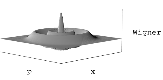
Figure 1: SHO Wigner Function for $n=4$

Figure 2: Wigner function for $n=4$, $r^{2}=x^{2}+p^{2}$

Figure 3: Probability density for $x$ for SHO, $n=4$

Figures 1 and 3 depict the Wigner function for the $n=4$ stationary state of the SHO. Because it only depends on $u$, it has the circular symmetry seen in Figure 1. Figure 3 therefore gives the Wigner profile for any straight line in phase space passing through the origin.

The classical SHO with this symmetry follows a circular trajectory in phase space, centered on the origin. The naive expectation might be then that the Wigner function, describing the corresponding quantum state, is a spread-out version of this; a single, circular ridge located above the corresponding classical phase path. The Figures show that only part of the Wigner function looks like that. There are oscillations in $\rho$, and it even goes into negative values. This means it is not a true probability distribution; it is instead called a quasi-probability distribution.

This feature partly explains why deformation quantization is less popular than other formalisms of quantum mechanics. We stress again, however, that it reproduces all the predictions of the more familiar operator methods. For instance, Figure 3 plots the probability density ${\cal P}(x)$ against $x$ (it could also be ${\cal P}(x)$ against $p$, because of symmetry), found using (38). The curve is identical to that found from the state vector solving Schrodinger’s equation. It is also true that expectation values of operators, such as $X^{m}P^{n}$, calculated using (40), agree perfectly with those calculated in the more familiar formulations of quantum mechanics.

6 Conclusion

Deformation quantization is another way to do quantum mechanics. It has some strange features, such as a quasi-probability distribution, and an exotic way of multiplying functions, the $\star$-product. But it is perfectly consistent, and its predictions agree with those made using other formulations of quantum mechanics. Furthermore, it is independent of the other formulations. On another planet, it might be the method of doing quantum mechanics discovered first! [11]

We believe that studying it, along with other quantum methods, deepens understanding of quantum physics. For example, writing $FG$ might allow one to slip into thinking that the product of operators is similar to an ordinary product of functions. But the $\star$-product simulates the product of operators, in the way discussed above, and so eqn. (3) makes clear that products of operators are tricky things.

Deformation quantization is a bit of a well-kept secret, especially at the undergraduate level. We hope our brief discussion of it here can serve as a gentle introduction to the subject for upper-level undergraduates, and perhaps others.

Acknowledgments This work was completed while JH and BW were undergraduate summer research assistants at the University of Lethbridge. For funding we thank the University of Lethbridge Research Fund and NSERC of Canada.

References

-
[1]
D.B. Fairlie, “The formulation of quantum mechanics in terms of
phase space functions,” Proc. Cambridge Phil. Soc. 60,
581-586 (1964),
M.V. Berry, “Semi-classical mechanics in phase space: a study of Wigner’s function,” Philos. Trans. Roy. Soc. London Ser. A 287, 237-271 (1977),
N.L. Balazs, B.K. Jennings, “Wigner’s function and other distribution functions in mock phase spaces,” Phys. Rept. 104, 347–391 (1984),
M. Hillery, R. O’Connell, M. Scully, E. Wigner, “ Distribution functions in physics: fundamentals,” Phys. Rept. 106, 121–167 (1984),
H.-W. Lee, “Theory and applications of the quantum phase-space distribution functions,” Phys. Rept. 259, 147-211 (1995),
C. Zachos, “Deformation quantization: quantum mechanics lives and works in phase-space,” Int. J. Mod. Phys. A17 (3), 297-316 (2002) [hep-th/0110114] - [2] F. Bayen, M. Flato, C. Fronsdal, A. Lichnerowicz, D. Sternheimer, “Deformation theory and quantization I, II,” Ann. Phys. (N.Y.) 111, 61, 111 (1978)
- [3] A. Hirshfeld, P. Henselder, “Deformation quantization in the teaching of quantum mechanics,” Am. J. Phys. 70, 537 (2002) [quant-ph/0208163]
- [4] L. Ballentine, Quantum mechanics: a modern development (World Scientific, 1998), chapter 15
- [5] M. R. Douglas, C. Hull, “D-branes and the noncommutative torus,” J. High Energy Phys. 9802, 008 (1998) [hep-th/9711165]
- [6] V. Schomerus, “D-branes and deformation quantization,” J. High Energy Phys. 9906, 030 (1999) [hep-th/9903205]
- [7] M. Kontsevich, “Deformation quantization of Poisson manifolds,” q-alg/9709040 (1997)
- [8] C. Cohen-Tannoudji, B. Diu, F. Laloë, Quantum mechanics (Wiley, 1977), vol. I, complement EIII
- [9] H. Goldstein, Classical Mechanics (Addison-Wesley, 1980), 2nd ed., sections 9-4 & 9-5
- [10] T. Curtright, D. Fairlie, C. Zachos, “Features of time-independent Wigner functions,” Phys. Rev. D58 (2), 025002-025017 (1998) [hep-th/9711183]
- [11] C. Zachos, “Deformation Quantization: Quantum Mechanics Lives & Works in Phase-Space,” Fermilab Colloquium Lecture, August 1, 2001; streaming video available from www.fnal.gov/faw/seminars.html