The Extended Plane Wave Expansion Method in Three Dimensional Anisotropic Photonic Crystal

Abstract

In this paper, we extend the conventional plane wave expansion method in 3D anisotropic photonic crystal to be able to calculate the complex $\mathbf{k}$ even if permittivity and permeability are complex numbers or the functions of $\omega$. There are some tricks in the derivation process, so we show the process in detail. Besides, we also provide an example for testing and explaining, and we also compare the results with the band structure derived from conventional plane wave expansion method, then we finally find that there is a good consistency between them.

Recently, the researches of the properties of the photonic crystals (PCs) have aroused great interests, since the concept of the PCs has been proposed by Yablonovitch and John1 ; 2 ; 3 . Briefly speaking, PCs are periodically structured electromagnetic media, generally processing photonic band gap (PBG). Most of the studies stress the PBG structures with the use of conventional plane-wave expanded (PWE) method7 ; 8 . However, there are still many articles explore the influence of interface, such as the studies of transmission, reflection, and the penetration depth etc.9 ; 10 ; 11 ; 12 Furthermore, the penetration depth relates to the imaginary part of wave vector. As for the complex ${\bf k}$ calculation in 2D isotropic photonic crystals, we had sufficiently discussed about it in the last paper[13]. Now, this paper is to continue with the last one. Furthermore, the emphasis of this paper is put on the general formula, 3D anisotropic case, of extended plane wave expansion (EPWE) method.

Though the main part of the idea resembles in 2D isotropic case[13], the formula and derivative process are much more complicated than that in 2D isotropic case, because the basis of wave functions can not be treated as scalar functions, TE and TM modes in 2D isotropic case. However, the problem of the difficult part has been overcome and we will explain it in the following description. Besides, the eigenfunctions set derived from this EPWE method is completely the same as that derived from the conventional PWE method. So we have no qualms about the inaccuracy of the propagation modes between these two methods.

The system we discussed is periodically structured without charge $\rho$ and current $\mathbf{J}$. Therefore, according to Maxwell Equation, the magnetic field $\mathbf{H}(\mathbf{r})$ should obey

$$-\left(\mathbf{k+G}\right)\times\hat{\epsilon}_{\mathbf{G-G}^{\prime}}^{-1}\left(\mathbf{k+G}^{\prime}\right)\times\mathbf{H}_{\mathbf{G}^{\prime}}=\omega^{2}\hat{\mu}_{\mathbf{G-G}^{\prime}}\mathbf{H}_{\mathbf{G}^{\prime}},$$ (1)

where

$$\mathbf{H}(\mathbf{r}) =\sum\limits_{\mathbf{G}}\mathbf{H}_{\mathbf{G}}e^{i(\mathbf{k+G})\cdot\mathbf{r}},$$

$$\hat{\epsilon}(\mathbf{r}) =\sum\limits_{\mathbf{G}}\hat{\epsilon}_{\mathbf{G}}e^{i\mathbf{G}\cdot\mathbf{r}},$$

$$\hat{\mu}(\mathbf{r}) =\sum\limits_{\mathbf{G}}\hat{\mu}_{\mathbf{G}}e^{i\mathbf{G}\cdot\mathbf{r}},$$

$\mathbf{G}$ and $\mathbf{G}^{\prime}$ are the reciprocal lattice vectors, $\omega$ and $\mathbf{k}$ are the frequency and wave vector, $\hat{\epsilon}(\mathbf{r})$ and $\hat{\mu}(\mathbf{r})$ are the tensors of permittivity and permeability of which $\hat{\epsilon}_{\mathbf{G}}$ and $\hat{\mu}_{\mathbf{G}}$ are the Fourier expansion components, respectively.

Now, let us expand Eq.(1) directly through $\mathbf{\hat{x}}$,$\mathbf{\hat{y}}$ and $\mathbf{\hat{z}}$ directions

$$\mathbf{\hat{x}} \mathbf{:}$$

$$\left[\left(k+G\right)_{y}\epsilon_{zy}^{-1}\left(k+G^{\prime}\right)_{z}+\left(k+G\right)_{z}\epsilon_{yz}^{-1}\left(k+G^{\prime}\right)_{y}-\left(k+G\right)_{y}\epsilon_{zz}^{-1}\left(k+G^{\prime}\right)_{y}-\left(k+G\right)_{z}\epsilon_{yy}^{-1}\left(k+G^{\prime}\right)_{z}\right]H_{x}$$

$$+\left[\left(k+G\right)_{y}\epsilon_{zz}^{-1}\left(k+G^{\prime}\right)_{x}+\left(k+G\right)_{z}\epsilon_{yx}^{-1}\left(k+G^{\prime}\right)_{z}-\left(k+G\right)_{y}\epsilon_{zx}^{-1}\left(k+G^{\prime}\right)_{z}-\left(k+G\right)_{z}\epsilon_{yz}^{-1}\left(k+G^{\prime}\right)_{x}\right]H_{y}$$

$$+\left[\left(k+G\right)_{y}\epsilon_{zx}^{-1}\left(k+G^{\prime}\right)_{y}+\left(k+G\right)_{z}\epsilon_{yy}^{-1}\left(k+G^{\prime}\right)_{x}-\left(k+G\right)_{y}\epsilon_{zy}^{-1}\left(k+G^{\prime}\right)_{x}-\left(k+G\right)_{z}\epsilon_{yx}^{-1}\left(k+G^{\prime}\right)_{y}\right]H_{z}$$

$$=-\omega^{2}\left(\mu_{xx}H_{x}+\mu_{xy}H_{y}+\mu_{xz}H_{z}\right),$$ (2a)

$$\mathbf{\hat{y}} \mathbf{:}$$

$$\left[\left(k+G\right)_{z}\epsilon_{xy}^{-1}\left(k+G^{\prime}\right)_{z}+\left(k+G\right)_{x}\epsilon_{zz}^{-1}\left(k+G^{\prime}\right)_{y}-\left(k+G\right)_{z}\epsilon_{xz}^{-1}\left(k+G^{\prime}\right)_{y}-\left(k+G\right)_{x}\epsilon_{zy}^{-1}\left(k+G^{\prime}\right)_{z}\right]H_{x}$$

$$+\left[\left(k+G\right)_{z}\epsilon_{xz}^{-1}\left(k+G^{\prime}\right)_{x}+\left(k+G\right)_{x}\epsilon_{zx}^{-1}\left(k+G^{\prime}\right)_{z}-\left(k+G\right)_{z}\epsilon_{xx}^{-1}\left(k+G^{\prime}\right)_{z}-\left(k+G\right)_{x}\epsilon_{zz}^{-1}\left(k+G^{\prime}\right)_{x}\right]H_{y}$$

$$+\left[\left(k+G\right)_{z}\epsilon_{xx}^{-1}\left(k+G^{\prime}\right)_{y}+\left(k+G\right)_{x}\epsilon_{zy}^{-1}\left(k+G^{\prime}\right)_{x}-\left(k+G\right)_{z}\epsilon_{xy}^{-1}\left(k+G^{\prime}\right)_{x}-\left(k+G\right)_{x}\epsilon_{zx}^{-1}\left(k+G^{\prime}\right)_{y}\right]H_{z}$$

$$=-\omega^{2}\left(\mu_{yx}H_{x}+\mu_{yy}H_{y}+\mu_{yz}H_{z}\right),$$ (2b)

$$\mathbf{\hat{z}} \mathbf{:}$$

$$\left[\left(k+G\right)_{x}\epsilon_{yy}^{-1}\left(k+G^{\prime}\right)_{z}+\left(k+G\right)_{y}\epsilon_{xz}^{-1}\left(k+G^{\prime}\right)_{y}-\left(k+G\right)_{x}\epsilon_{yz}^{-1}\left(k+G^{\prime}\right)_{y}-\left(k+G\right)_{y}\epsilon_{xy}^{-1}\left(k+G^{\prime}\right)_{z}\right]H_{x}$$

$$+\left[\left(k+G\right)_{x}\epsilon_{yz}^{-1}\left(k+G^{\prime}\right)_{x}+\left(k+G\right)_{y}\epsilon_{xx}^{-1}\left(k+G^{\prime}\right)_{z}-\left(k+G\right)_{x}\epsilon_{yx}^{-1}\left(k+G^{\prime}\right)_{z}-\left(k+G\right)_{y}\epsilon_{xz}^{-1}\left(k+G^{\prime}\right)_{x}\right]H_{y}$$

$$+\left[\left(k+G\right)_{x}\epsilon_{yx}^{-1}\left(k+G^{\prime}\right)_{y}+\left(k+G\right)_{y}\epsilon_{xy}^{-1}\left(k+G^{\prime}\right)_{x}-\left(k+G\right)_{y}\epsilon_{xx}^{-1}\left(k+G^{\prime}\right)_{y}-\left(k+G\right)_{x}\epsilon_{yy}^{-1}\left(k+G^{\prime}\right)_{x}\right]H_{z}$$

$$=-\omega^{2}\left(\mu_{zx}H_{x}+\mu_{zy}H_{y}+\mu_{zz}H_{z}\right),$$ (2c)

where $\epsilon_{ij}$ and $\mu_{ij}$ are the abbreviations of $\hat{\epsilon}_{\mathbf{G-G}^{\prime},i,j}$ and $\hat{\mu}_{\mathbf{G-G}^{\prime},i,j}$, and $H_{i}$ is the abbreviation of $H_{\mathbf{G}^{\prime},i}$. When $\mathbf{k}$ is provided, Eq.(2) becomes an eigenvalue problem in which the eigenvalue is $\omega$ and is the conventional PWE method. Now, there comes up an interesting question that is whether $\mathbf{k}$ must be a vector of which the components are real numbers. The answer is ”No”, and we just need to do some modification on Eq.(2) to get the complex $\mathbf{k}$, because Eq.(2) is a 4 variables ($\mathbf{k}$ and $\omega$) equation.

In the beginning, two important things need discussing. First, the inner product of $(\mathbf{k+G})$ and Eq.(2) results in

$$\sum\limits_{\begin{subarray}{c}G^{\prime},i,j\\ i,j=x,y,z\end{subarray}}(k_{i}+G_{i})\mu_{\mathbf{G-G}^{\prime},i,j}H_{\mathbf{G}^{\prime},j}=0$$

which are the restriction functions of which the amount is $N$, meanwhile, $N$ is the amount of $\{G\}$ set. Therefore, the certain amount of the independent eigenfunctions in Eq.(2) is $2N$ not $3N$. That’s why we will get the fake eigenvalues which are $\omega^{2}=0$ if Eq.(2) is calculated as an eigenvalue equation directly.

To avoid this situation occurring in our method, the eigenvector we selected in our method is $\left(\begin{array}[c]{c}\mathbf{H}_{\mathbf{G}\perp}\\ \mathbf{\tilde{H}}_{\mathbf{G}\perp}\end{array}\right)$ not $\left(\begin{array}[c]{c}\mathbf{H}_{\mathbf{G}}\\ \mathbf{\tilde{H}}_{\mathbf{G}}\end{array}\right)$, where $\mathbf{H}_{\mathbf{G}\perp}$ and $\mathbf{H}_{\mathbf{G}}$ are $\left(\begin{array}[c]{c}H_{\mathbf{G},y}\\ H_{\mathbf{G},z}\end{array}\right)$ and $\left(\begin{array}[c]{c}H_{\mathbf{G},x}\\ \mathbf{H}_{\mathbf{G}\perp}\end{array}\right)$, $\mathbf{\tilde{H}}_{\mathbf{G}\perp}$ and $\mathbf{\tilde{H}}_{\mathbf{G}}$ are $k_{x}\mathbf{H}_{\mathbf{G}\perp}$ and $k_{x}\mathbf{H}_{\mathbf{G}}$, respectively.

Second, there are no $k_{x}^{2}H_{\mathbf{G}^{\prime},i}$ , $i=x,y,z$, and $k_{x}H_{\mathbf{G}^{\prime},x}$ in Eq.(2a), which is the $\mathbf{\hat{x}}$ component of Eq.(1), because the inner products of Eq.(1) and $\mathbf{\hat{x}}$ will cause the existence of just one $k_{x}$ or even no, and $(\mathbf{k}+\mathbf{G}\prime)\times\mathbf{H}_{\mathbf{G\prime}}$ part will restrict the existence of $k_{x}H_{\mathbf{G,}x}$.

Therefore, the treatment of $\mathbf{\hat{x}}$ component will be different from $\mathbf{\hat{y}}$ and $\mathbf{\hat{z}}$ components. The following is the detail derivation process:

First of all, the $\mathbf{\hat{y}}$ and $\mathbf{\hat{z}}$ components of Eq.(2) can be written as a matrix formula

$$\left[\mathbf{\hat{B}}_{1}\vdots\mathbf{\hat{B}}_{2}\vdots\mathbf{\hat{C}}_{1}\vdots\mathbf{\hat{C}}_{2}\right]\left(\begin{array}[c]{c}\mathbf{H}_{\mathbf{G}}\\ \mathbf{\tilde{H}}_{\mathbf{G}}\end{array}\right)=\mathbf{\hat{A}}\left(k_{x}\mathbf{\tilde{H}}_{\mathbf{G\perp}}\right),$$

and its expansion type is

$$\mathbf{\hat{B}}_{1}H_{\mathbf{G},x}+\mathbf{\hat{C}}_{1}\tilde{H}_{\mathbf{G},x}+\left(\mathbf{\hat{B}}_{2}\vdots\mathbf{\hat{C}}_{2}\right)\left(\begin{array}[c]{c}\mathbf{H}_{\mathbf{G}\perp}\\ \mathbf{\tilde{H}}_{\mathbf{G}\perp}\end{array}\right)=k_{x}\mathbf{\hat{A}}\left(\mathbf{\tilde{H}}_{\mathbf{G\perp}}\right),$$ (5)

where $\mathbf{\hat{A}}$, $\mathbf{\hat{B}}_{1}$, $\mathbf{\hat{B}}_{2}$, $\mathbf{\hat{C}}_{1}$, $\mathbf{\hat{C}}_{2}$ are $2N\times 2N$, $2N\times N$, $2N\times 2N$, $2N\times N$ and $2N\times 2N$ matrices and their elements will be illustrated in Appendix.

As regards the $\mathbf{\hat{x}}$ component of Eq.(2), we can write in another form which is different from $\mathbf{\hat{y}}$ and $\mathbf{\hat{z}}$ components of Eq.(2). Thus the matrix form of Eq.(2a) is

$$\left(\mathbf{\hat{E}}_{1}\vdots\mathbf{\hat{E}}_{2}\right)\left(\mathbf{H}_{\mathbf{G}}\right)=\mathbf{\hat{D}}\left(\mathbf{\tilde{H}}_{\mathbf{G\perp}}\right),$$ (6)

where $\mathbf{\hat{D}}$, $\mathbf{\hat{E}}_{1}$, $\mathbf{\hat{E}}_{2}$ are $N\times 2N$, $N\times N$, $N\times 2N$ and their elements are also in Appendix.

From Eq.(4) we obtain

$$H_{\mathbf{G},x} =-\mathbf{\hat{E}}_{1}^{-1}\mathbf{\hat{E}}_{2}\mathbf{H}_{\mathbf{G\perp}}+\mathbf{\hat{E}}_{1}^{-1}\mathbf{\hat{D}\tilde{H}}_{\mathbf{G\perp}},$$ (7a)

$$\tilde{H}_{\mathbf{G},x} =-\mathbf{\hat{E}}_{1}^{-1}\mathbf{\hat{E}}_{2}\mathbf{\tilde{H}}_{\mathbf{G\perp}}+k_{x}\mathbf{\hat{E}}_{1}^{-1}\mathbf{\hat{D}\tilde{H}}_{\mathbf{G\perp}},$$ (7b)

where Eq.(5b) is the production of Eq.(5a) multiplied by $k_{x}$. A combination of Eqs.(3) and (5) yields

$$k_{x}\mathbf{\tilde{H}}_{\mathbf{G\perp}} =\left[\mathbf{\hat{A}-\hat{C}}_{1}\mathbf{\hat{E}}_{1}^{-1}\mathbf{\hat{D}}\right]^{-1}\left[\left(\mathbf{\hat{B}}_{1}\mathbf{\hat{E}}_{1}^{-1}\right)\left(-\mathbf{\hat{E}}_{2}\vdots\mathbf{\hat{D}}\right)+\left(\mathbf{\hat{C}}_{1}\mathbf{\hat{E}}_{1}^{-1}\right)\left(\O\vdots-\mathbf{\hat{E}}_{2}\right)+\left(\mathbf{\hat{B}}_{2}\vdots\mathbf{\hat{C}}_{2}\right)\right]\left(\begin{array}[c]{c}\mathbf{H}_{\mathbf{G}\perp}\\ \mathbf{\tilde{H}}_{\mathbf{G}\perp}\end{array}\right)$$

$$\equiv\mathbf{\hat{F}}\left(\begin{array}[c]{c}\mathbf{H}_{\mathbf{G}\perp}\\ \mathbf{\tilde{H}}_{\mathbf{G}\perp}\end{array}\right),$$

where $\mathbf{\hat{F}}$ is a $2N\times 4N$ matrix. Considering the equation above with $k_{x}\mathbf{H}_{\mathbf{G\perp}}=\mathbf{\tilde{H}}_{\mathbf{G\perp}}$, we finally have an equation

$$\left(\begin{array}[c]{c}\;\O\;\vdots\;\mathbf{I}\\ \cdots\cdots\\ \mathbf{F}\end{array}\right)\left(\begin{array}[c]{c}\mathbf{H}_{\mathbf{G}\perp}\\ \mathbf{\tilde{H}}_{\mathbf{G}\perp}\end{array}\right)=k_{x}\left(\begin{array}[c]{c}\mathbf{H}_{\mathbf{G}\perp}\\ \mathbf{\tilde{H}}_{\mathbf{G}\perp}\end{array}\right),$$ (15)

which is an $k_{x}$ eigenvalue equation, and the order of eigenfunction $\left(\begin{array}[c]{c}\mathbf{H}_{\mathbf{G}\perp}\\ \mathbf{\tilde{H}}_{\mathbf{G}\perp}\end{array}\right)$ is $4N$. In addition, $\O$ and ${\bf I}$ are $2N\times 2N$ zero matrix and identity matrix, alternatively.

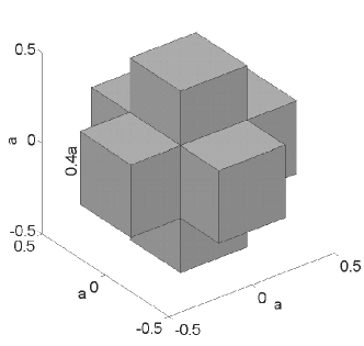
Figure 1: The schematic view of a cubic unit cell in which three GaAs square rods cross together from the ${\bf\hat{x}}$, ${\bf\hat{y}}$ and ${\bf\hat{z}}$ direction. The lattice constant, width of square rods and $\epsilon$ of GaAs are $a$, $0.4a$ and $11.43\epsilon_{0}$, respectively.

For testing this method, we use an Intel centrino 1.4G, 512 MB RAM with matlab code published on mathworks website to run an isotropic simple cubic case in which the GaAs square rods — their widths are $0.4a$, and $a$ is the lattice constant — cross together from $\mathbf{\hat{x}}$,$\mathbf{\hat{y}}$ and $\mathbf{\hat{z}}$ direction in the vacuum. In this system the permittivity $\epsilon$ of GaAs and vacuum are $11.43\epsilon_{0}$ and $\epsilon_{0}$, alternatively, and the permeability $\mu$ is $\mu_{0}$ everywhere. You can see its structure in Fig.(1) and calculation results in Fig.(2). We spent about 6 hours on getting Figs.(2b) and (2c) when using 729 $\{\mathbf{G}\}$ and taking $17$ $k_{y}$ points from $0$ to $\frac{\pi}{a}$ to accomplish the calculation. As regards Fig.(2a), it is the band structure which is derived from Eq.(2) and used to compare with our method. In Fig.(2a), we can find that $\omega=0.2\frac{2\pi c}{a}$ is not located in band gap, so such kind of condition should also appeared in our method when we choose the same $\omega$ to plot the contour line or surface. Figure (2b) in which $\omega=0.2\frac{2\pi c}{a}$ , $k_{z}=0$ and $k_{y}$ scanned from $-\frac{\pi}{a}$ to $\frac{\pi}{a}$ is the figure of real value solution of $k_{x}$ derived from Eq.(6). When Fig.(2a) compares with Fig.(2b), we will find out the width of contour in Fig.(2b) equals the width of $\mathbf{X}\rightarrow{\bf\Gamma}$ region in Fig.(2a).

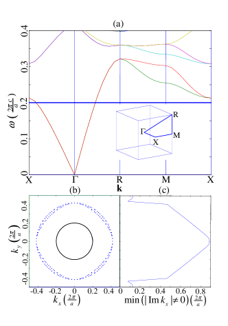
Figure 2: The numerical results of Fig.1. (a) is the band structure derived from Eq.(2) and in which the bold line is the $\omega=0.2\frac{2\pi c}{a}$ line. (b) and (c) are the equal frequency contour line of propagation modes in k space and the $\min(|\operatorname{Im}(k_{x})|\neq 0)$ vs. $k_{y}$ figure, alternatively. The circle in (b) denotes the incident light of which $\omega=0.2\frac{2\pi c}{a}$. Both of them are derived from Eq.(6) when $\omega=0.2\frac{2\pi c}{a}$, $k_{z}=0$ and $k_{y}$ is scanned from $-\frac{\pi}{a}$ to $\frac{\pi}{a}$.

Besides, we can find that there are two propagation modes toward right when $k_{y}$ is a fixed number in Fig.(2b). These modes are similar to TE and TM modes in 2D isotropic PC, however, they can not be distinguished in 3D PC, we just plot them directly. Furthermore, $C_{4}^{1}$ symmetry exists in Fig.(2b) but not in the figure of real part of complex $k_{x}$. The reason is the real number solutions of $k_{x}$ are the $k_{x}$ of the propagation modes which are the solutions of bulk system in which the $C_{4}^{1}$ symmetry exist. However, the above is not correct when $k_{x}$ are complex numbers, because the complex means that there is an interface destroying the $C_{4}^{1}$ symmetry and facing $\mathbf{\hat{x}}$ direction in the system as well. Therefore, all the evanescent modes of which $k_{x}$ are complex numbers just exist near the interface and their penetration depths correspond to $2\pi/\left|\operatorname{Im}(k_{x})\neq 0\right|$ owing to $e^{i\mathbf{k\cdot r}}=e^{i\mathbf{k}^{R}\mathbf{\cdot r}}e^{i\mathbf{k}_{x}^{I}x}$, where $R$ and $I$ denote real and imaginary parts, alternatively. The most remarkable one of the complex $k_{x}$ relates to the longest penetration depth denoted as $\lambda_{LPD}\left(k_{y},k_{z},\omega\right)$, because almost nothing but the propagation modes can exist in this system when the distance from the detecting position to the interface is larger than $\lambda_{LPD}\left(k_{y},k_{z},\omega\right)$. Therefore, a semi-infinite system can be treated as two individual regions: surface and bulk regions, all the evanescent modes just exist in the surface region of which the width is $\lambda_{S}$ definded as $\max\left(\lambda_{LPD}\left(k_{y},k_{z},\omega_{0}\right)\right)$, where $\omega_{0}$ is a fixed frequency. For a finite size PC, if the effect of corner is not important, $\lambda_{S}$ decides the smallest size of PC. If the size is smaller than the smallest one, the system no longer can be treated as a periodic structured media. Figure(2c) is the figure of $a/\lambda_{LPD}$ vs. $k_{y}$ at $\omega=0.2\frac{2\pi c}{a}$. This figure indicates that the $a/\lambda_{LPD}$ drops to zero quickly when $k_{y}$ is located at the edge of contour in Fig.(2b). This kind of situation arises while the state located at the edge of contour changes from propagation mode to evanescent mode. Besides, because $|k_{y}|\leq 0.2\frac{2\pi}{a}$ when the incident light is a propagation mode in vacuum, we can find that $a/\lambda_{LPD}>0.7$. Therefore, the longest penetration depth is $a/0.7$ for all incident light perpendicular to $\mathbf{\hat{z}}$ direction.

In conclusion, because Eq.(6) is a $k_{x}$ eigenvalue equation when $\omega$, $k_{y}$ and $k_{z}$ are provided, the $\omega$ can be a real number at any time, and $\epsilon$ and $\mu$ can be the function of $\omega$, $k_{y}$ and $k_{z}$ or complex tensors. In addition, since most of $k_{x}$ are complex numbers, the minimum of $\left|\operatorname{Im}(k_{x})\neq 0\right|$ must exist, and this value will decide how large a PC is able to treated as a single crystal if the influence of corner is not important. Therefore, one of the issues we proceed to research is the influence of corner. We thank Prof. Ping Shen for his opinion to excite us to find out the 3D formula EPWE method.

I Appendix

The $\epsilon_{ij}$ shown as below is the abbreviation of $\epsilon_{{\bf G}-{\bf G}^{\prime},ij}$.

$${\bf A}= \left(\begin{array}[]{cc}\epsilon^{-1}_{zz}&-\epsilon^{-1}_{zy}\\ -\epsilon^{-1}_{yz}&\epsilon^{-1}_{yy}\\ \end{array}\right),$$

$$B_{1,11}= G_{x}\epsilon^{-1}_{zz}(k+G^{\prime})_{y}+(k+G)_{z}\epsilon^{-1}_{xy}(k+G^{\prime})_{z}-$$

$$G_{x}\epsilon^{-1}_{zy}(k+G^{\prime})_{z}-(k+G)_{z}\epsilon^{-1}_{xz}(k+G^{\prime})_{y}+\omega^{2}\mu_{yx},$$

$$B_{1,21}= G_{x}\epsilon^{-1}_{yy}(k+G^{\prime})_{z}+(k+G)_{y}\epsilon^{-1}_{xz}(k+G^{\prime})_{y}-$$

$$G_{x}\epsilon^{-1}_{yz}(k+G^{\prime})_{y}-(k+G)_{y}\epsilon^{-1}_{xy}(k+G^{\prime})_{z}+\omega^{2}\mu_{zx},$$

$$B_{2,11}= G_{x}\epsilon^{-1}_{zx}(k+G^{\prime})_{z}+(k+G)_{z}\epsilon^{-1}_{xz}G_{x}^{\prime}-$$

$$G_{x}\epsilon^{-1}_{zz}G_{x}^{\prime}-(k+G)_{z}\epsilon^{-1}_{xx}(k+G^{\prime})_{z}+\omega^{2}\mu_{yy},$$

$$B_{2,12}= G_{x}\epsilon^{-1}_{zy}G_{x}^{\prime}+(k+G)_{z}\epsilon^{-1}_{xx}(k+G^{\prime})_{y}-$$

$$G_{x}\epsilon^{-1}_{zx}(k+G^{\prime})_{y}-(k+G)_{z}\epsilon^{-1}_{xy}G_{x}^{\prime}+\omega^{2}\mu_{yz},$$

$$B_{2,21}= G_{x}\epsilon^{-1}_{yz}G_{x}^{\prime}+(k+G)_{y}\epsilon^{-1}_{xx}(k+G^{\prime})_{z}-$$

$$G_{x}\epsilon^{-1}_{yx}(k+G^{\prime})_{z}-(k+G)_{y}\epsilon^{-1}_{xz}G_{x}^{\prime}+\omega^{2}\mu_{zy},$$

$$B_{2,22}= G_{x}\epsilon^{-1}_{yx}(k+G^{\prime})_{y}+(k+G)_{y}\epsilon^{-1}_{xy}G_{x}^{\prime}-$$

$$G_{x}\epsilon^{-1}_{yy}G_{x}^{\prime}-(k+G)_{y}\epsilon^{-1}_{xx}(k+G^{\prime})_{y}+\omega^{2}\mu_{zz},$$

$$C_{1,11}= \epsilon^{-1}_{zz}(k+G^{\prime})_{y}-\epsilon^{-1}_{zy}(k+G^{\prime})_{z},$$

$$C_{1,21}= \epsilon^{-1}_{yy}(k+G^{\prime})_{z}-\epsilon^{-1}_{yz}(k+G^{\prime})_{y},$$

$$C_{2,11}= \epsilon^{-1}_{zx}(k+G^{\prime})_{z}+(k+G)_{z}\epsilon^{-1}_{xz}-\epsilon^{-1}_{zz}(G_{x}+G_{x}^{\prime}),$$

$$C_{2,12}= \epsilon^{-1}_{zy}(G_{x}+G_{x}^{\prime})-\epsilon^{-1}_{zx}(k+G^{\prime})_{y}-(k+G)_{z}\epsilon^{-1}_{xy},$$

$$C_{2,21}= \epsilon^{-1}_{yz}(G_{x}+G_{x}^{\prime})-\epsilon^{-1}_{yx}(k+G^{\prime})_{z}-(k+G)_{y}\epsilon^{-1}_{xz},$$

$$C_{2,22}= \epsilon^{-1}_{yx}(k+G^{\prime})_{y}+(k+G)_{y}\epsilon^{-1}_{xy}-\epsilon^{-1}_{yy}(G_{x}+G_{x}^{\prime}),$$

$$D_{11}= (k+G)_{z}\epsilon^{-1}_{yz}-(k+G)_{y}\epsilon^{-1}_{zz},$$

$$D_{12}= (k+G)_{y}\epsilon^{-1}_{zy}-(k+G)_{z}\epsilon^{-1}_{yy},$$

$$E_{1}= (k+G)_{y}\epsilon^{-1}_{zy}(k+G^{\prime})_{z}+(k+G)_{z}\epsilon^{-1}_{yz}(k+G^{\prime})_{y}-$$

$$(k+G)_{y}\epsilon^{-1}_{zz}(k+G^{\prime})_{y}-(k+G)_{z}\epsilon^{-1}_{yy}(k+G^{\prime})_{z}+\omega^{2}\mu_{xx},$$

$$E_{2,11}= (k+G)_{y}\epsilon^{-1}_{zz}G_{x}^{\prime}+(k+G)_{z}\epsilon^{-1}_{yx}(k+G^{\prime})_{z}-$$

$$(k+G)_{y}\epsilon^{-1}_{zx}(k+G^{\prime})_{z}-(k+G)_{z}\epsilon^{-1}_{yz}G_{x}^{\prime}+\omega^{2}\mu_{xy},$$

$$E_{2,12}= (k+G)_{z}\epsilon^{-1}_{yy}G_{x}^{\prime}+(k+G)_{y}\epsilon^{-1}_{zx}(k+G^{\prime})_{y}-$$

$$(k+G)_{z}\epsilon^{-1}_{yx}(k+G^{\prime})_{y}-(k+G)_{y}\epsilon^{-1}_{zy}G_{x}^{\prime}+\omega^{2}\mu_{xz}.$$

References

(1) C. M. Surko and P. Kolodner, Phys. Rev. Lett. 58, 2055 (1987); S.
John, Phys. Rev. Lett. 58, 2486 (1987).
(2) E.Yablonovitch, T. J. Gmitter, R. D. Meade, A. M. Rappe, K. D. Brommer, and J. D. Joannopoulos, Phys. Rev. Lett. 67,
3380(1991).
(3) E.Yablonovitch, T. J. Gmitter, and K. M.Leung, Phys. Rev.
Lett. 67, 2295 (1991).
(4) K. Sakoda, Optical Properties of Photonic Crystals
(Springer-Verlag, 2001).
(5) Z. Y. Li, B. Y. Gu, and G. Z. Yang, Phys. Rev. Lett. 81,
2574 (1998); Eur. Phys. J. B 11, 65 (1999).
(6) K. Sakoda, Phys. Rev. B 52, 8992 (1995).
(7) J. B. Pendry, J. Mod. Opt. 41, 209 (1994).
(8) B. Gralak, S. Enoch and G. Tayeb, J. Opt. Soc. Am. A 17, 1012-1020 (2000).
(9) J. B. Pendry and A. MacKinnon, Phys. Rev. Lett. 69, 2772
(1992).
(10) Y. C. Hsue and T. J. Yang, arXiv:physics/0307150 (2003), Y. C. Hsue and T. J. Yang, Solid State Comm. 129, 475 (2004) and Y. C. Hsue and T. J. Yang, Phys. Rev. E, 2004 accepted.