A COMPARISON OF INCOMPRESSIBLE LIMITS FOR RESISTIVE PLASMAS.

Abstract

The constraint of incompressibility is often used to simplify the magnetohydrodynamic (MHD) description of linearized plasma dynamics because it does not affect the ideal MHD marginal stability point. In this paper two methods for introducing incompressibility are compared in a cylindrical plasma model: In the first method, the limit $\gamma\rightarrow\infty$ is taken, where $\gamma$ is the ratio of specific heats; in the second, an anisotropic mass tensor $\mathbf{\rho}$ is used, with the component parallel to the magnetic field taken to vanish, $\rho_{\parallel}\rightarrow 0$. Use of resistive MHD reveals the nature of these two limits because the Alfvén and slow magnetosonic continua of ideal MHD are converted to point spectra and moved into the complex plane. Both limits profoundly change the slow-magnetosonic spectrum, but only the second limit faithfully reproduces the resistive Alfvén spectrum and its wavemodes. In ideal MHD, the slow magnetosonic continuum degenerates to the Alfvén continuum in the first method, while it is moved to infinity by the second. The degeneracy in the first is broken by finite resistivity. For numerical and semi-analytical study of these models, we choose plasma equilibria which cast light on puzzling aspects of results found in earlier literature.

.

1 Introduction

We devote our attention to the ideal and resistive MHD models, which despite their dramatic simplification of plasma behaviour, are crucial to the design and operation of controlled fusion devices and are at the core of many astrophysical plasma models. Simplified models such as these have utility if they can be used to make testable predictions or if they yield insight into the internal processes of a system. We test two variants of incompressible resistive MHD with these criteria in mind. The starting point for the analysis of most plasma models is an understanding of the wavemodes that arise: this provides information about the linear response and stability of the system and provides a basis for much nonlinear analysis. We focus on the linear behaviour of the plasma in this paper. For the resistive MHD model, which includes dissipation, the wavemodes are non-normal: a full picture of linear plasma behaviour requires an analysis of the transient behaviour of the system, as well as the eigenvalue analysis which predicts asymptotic behaviours over long time scales. These are closely related via pseudospectral methods [1]. In this paper we restrict attention to eigenvalue analysis.

For many plasmas of physical interest it is true that the resistive term is small: typically this is quantified by a large magnetic Reynolds number. It might have been expected that for small enough resistivity, the resistive MHD model could simply be treated as a perturbation of the ideal MHD model. However, the change induced is actually a singular perturbation, which introduces higher spatial derivatives. One of the interesting effects of this property is that eigenfrequencies in the ideal model are not necessarily approached by the eigenfrequencies of any resistive modes, even for vanishingly small resistivity.

Many papers have been published on the stable resistive MHD spectrum and several of the early papers ([2]- [6]) focused on cylindrical models. These papers have established certain generic features of the resistive spectrum. The resistive spectrum is discrete, unlike the ideal MHD spectrum which has continua: on some intervals, every frequency corresponds to a generalised wavemode. In the resistive spectrum, a large number of fully complex eigenfrequencies can be found, and in general these lie along loci, or lines, on the complex plane. Generally as the resistivity is decreased to zero these lines become densely populated with eigenvalues.

Resistive MHD is a simple closure of the full kinetic equations, and as a result the plasma dynamics parallel to the magnetic field lines are often quite poorly represented [7]. For Alvénic modes, which do not strongly compress the plasma, these parallel dynamics are generally unimportant. However, for the slow and fast magnetoacoustic waves, the parallel dynamics and the effects of compressibility are important; these waves are not necessarily well modelled by resistive MHD.

It is possible to find the compressible resistive MHD spectrum numerically (as in [5]) and ignore the slow and fast magnetoacoustic waves that are present. On the other hand, there are approaches which promise to isolate the Alfvénic portion of the spectrum and simplify the analysis. We present two of these incompressible approximations, in which the predicted motions of the plasma satisfy $\nabla\mbox{\boldmath$\cdot$}\mathbf{v}=0$ (at least approximately). One approach is to artificially set the ratio of specific heats $\gamma$ to infinity (as in [4] and [6]). In the other, an anisotropic mass tensor $\mathbf{\rho}$ is used, with the component parallel to the magnetic field taken to vanish, $\rho_{\parallel}/\rho_{\perp}\rightarrow 0$. With this density tensor, ideal eigenmodes are incompressible, but to ensure exact incompressibility for resistive eigenmodes $\gamma$ must again be set to $\infty$. We can view these models as the extreme cases of a generalised resistive MHD model with two parameters, $\gamma$ and $\rho_{\parallel}/\rho_{\perp}$. The two extreme cases are not equivalent, and the resulting spectra are qualitatively different. We investigate these two methods, and compare them with the compressible resistive MHD model. We specialise to equilibria with zero background flow. Note that $\gamma\rightarrow\infty$ may be physically appropriate for particular conductive fluids and plasmas with $\beta>>1$.

First, we examine the plane waves of the homogeneous incompressible MHD model. Then we evaluate spectra in a simple cylindrical equilibrium for varying values of $\gamma$, and with and without an artificial anisotropic density. This illustrates the transition between the compressible and incompressible cases. We then discuss the spectra of more general plasma configurations. A WKB analysis of a generic incompressible model is then undertaken in order to understand the features of these spectra and to verify the numerics. We begin by solving the dispersion relation. Then the singular features of this function are explored by reducing it to a simpler form. To complete the groundwork for semi-analytic calculations, the behaviour of the wave equation near these singular points is examined. Finally, we use our WKB analysis to find the spectrum of an example case.

2 Wavemodes in incompressible MHD limits

The first step in the analysis of these incompressible limits is a determination of the wavemodes in a simple homogeneous plasma. To this end we follow [7] and derive wave frequencies. We begin by considering a wave with wavevector at some angle to the magnetic field $\mathbf{B}=B_{0}\hat{z}$, so $\mathbf{k}=k_{\parallel}\hat{z}+k_{\perp}\hat{x}$, travelling in a plasma with sound speed $V_{s}=(\gamma p_{0}/\rho_{0})^{1/2}$ and Alfvén speed $V_{a}=(B_{0}^{2}/\mu_{0}\rho_{0})^{1/2}$. We recover the Alfvén spectrum:

$$\omega_{A}^{2}=k_{\parallel}^{2}{V_{a}}^{2},$$ (1)

and also two other solutions to the plasma equations:

$$\omega_{\pm}^{2}=\frac{1}{2}k^{2}({V_{a}}^{2}+{V_{s}}^{2}+\frac{\rho_{\parallel}-\rho_{\perp}}{\rho_{\parallel}k^{2}}k_{\parallel}^{2}V_{s}^{2})\left(1\pm(1-\alpha^{2})^{\frac{1}{2}}\right),$$ (2)

where

$$\alpha^{2}=\frac{4\rho_{\perp}k_{\parallel}^{2}{V_{a}}^{2}{V_{s}}^{2}}{k^{2}\rho_{\parallel}({V_{a}}^{2}+{V_{s}}^{2}+\frac{\rho_{\parallel}-\rho_{\perp}}{\rho_{\parallel}k^{2}}k_{\parallel}^{2}V_{s}^{2})^{2}}.$$ (3)

In low-$\beta$ compressible plasmas, $\omega_{+}$ corresponds to the fast magnetoacoustic wave, and $\omega_{-}$ to the slow magnetoacoustic wave.

In the limit $\gamma\rightarrow\infty$ (with $\rho_{\parallel}/\rho_{\perp}=1$) we find $\omega_{+}^{2}\rightarrow\infty$ and $\omega_{-}^{2}\rightarrow k_{\parallel}^{2}{V_{a}}^{2}$, so that the slow-mode is now degenerate with the Alfvén mode. In more general plasma configurations, the slow and the Alfvén wavemodes still occur at very similar frequencies, and therefore can be strongly mixed. We show this does occur, so that generic spectra determined are composed of an unphysical combination of these types of wavemodes. In the limit $\rho_{\parallel}/\rho_{\perp}\rightarrow 0$ we again have $\omega_{+}\rightarrow\infty$, but $\omega_{-}^{2}\rightarrow k^{2}V_{a}^{2}+k_{\perp}^{2}V_{s}^{2}$, which is slightly larger than the fast magnetoacoustic frequency. In this case we have suppressed the slow magnetoacoustic waves.

If we set $\rho_{\parallel}/\rho_{\perp}\rightarrow 0$, we can show from the linearised equations that for general resistive MHD wavemodes $\rho_{\parallel}\rightarrow 0$ implies:

$$\mathbf{B}_{0}\mbox{\boldmath$\cdot$}\mbox{\boldmath$\nabla$}(\mbox{\boldmath$\nabla\cdot$}\mathbf{v})=-\frac{\mbox{\boldmath$\nabla$}P_{0}\mbox{\boldmath$\cdot$}\mbox{\boldmath$\nabla\times$}(\eta\mathbf{j})}{(\gamma P_{0})},$$ (4)

where $B_{0}$ and $P_{0}$ are the equilibrium field and pressure, $\eta$ is the resistivity and $\mathbf{j}$ and $\mathbf{v}$ are the perturbed current and velocity. So for the ideal case ($\eta=0$) we have that $\mbox{\boldmath$\nabla\cdot$}\mathbf{v}$ is a constant on all irrational surfaces, and, by continuity, for finite toroidal or poloidal mode number, we must have $\mbox{\boldmath$\nabla\cdot$}\mathbf{v}=0$. In the resistive case, we have small $\eta$, but possibly large $d/dr$ so that resistive modes are not strictly incompressible. However, if we also require $\gamma\rightarrow\infty$ then the resistive modes are strictly incompressible.

3 Numerical results of varying incompressibility

In order to show the effect of incompressibility on the resistive MHD spectrum, we solved the compressible, resistive MHD equations numerically. We use a code based on the description in [8].

We examine a cylindrical, zero-shear model case, as described in [6] , with $\beta\approx 4\%$. The incompressibility is explored by varying $\gamma$ in the range $1$ – $1000$. The incompressible limits correspond to $\gamma\rightarrow\infty$, but in this case $\gamma\simeq 1000$ is high enough to demonstrate the limit. We define the magnetic Reynolds number $S=\tau_{R}/\tau_{A}$ where $\tau_{A}$ and $\tau_{R}$ are the Alfvén and resistive timescales. For a cylinder of radius $r_{p}$ we have $\tau_{A}=r_{p}(\mu_{0}\rho)^{1/2}/B_{z}$, and $\tau_{R}=r_{p}^{2}\mu_{0}/\eta_{0}$. The magnetic field perturbations are of the form $\mathbf{b}=\exp\left(im\theta-i\kappa z/r_{p}-i\omega t\right)\mathbf{b}\left(r\right)$, with $\kappa=nr_{p}/R$, by analogy with the toroidal case $R$ can be interpreted in the sense that $2\pi R$ is the length of the plasma column and $n$ is the ‘toroidal’ mode number. We have $\beta\approx 4\%$, which allows the slow-mode spectrum to be shown on the same scale as the Alfvén spectrum in the compressible case. The resulting spectra are shown in figure 1. For this case $m=1$, $\kappa=0.35$, $nq=1.2$ and $S=1\times 10^{4}$. Note that figure 1(e) corresponds to the limit $\gamma\rightarrow\infty$ and figure 1(f) corresponds to the limit $\rho_{\parallel}/\rho_{\perp}\rightarrow 0$.

In these cases the ideal Alfvén continuum degenerates to a point, at ${\omega}_{A}=0.057$, but the ideal slow continuum is finite in extent because of pressure and field strength variation across the plasma. The slow continuum extends to the origin because the pressure is taken to be zero at the plasma boundary. Note the fork structure seen for the slow modes near the origin of figure 1(a). This fork structure is lost as $\gamma$ is increased [figures 1(b)– (e)]. Finally, as $\gamma\rightarrow\infty$, most of the mode frequencies are in the vicinity of a semicircle of radius $\omega_{A}$ on the complex plane. From the figure, we see that there are many more modes near $\omega_{A}$ in the $\gamma\rightarrow\infty$ model, than in the more physical compressible model. It has been shown in [6] that for this incompressible case wavemodes are eigenfunctions of helicity and none of the modes correspond directly to physical compressible wavemodes. In figure 1(e), the two loci of eigenvalues correspond to wavemodes of opposite helicity.

For the $\rho_{\parallel}/\rho_{\perp}\rightarrow 0$ model, we find a spectrum [figure 1(f)] very similar to the compressible spectrum in figure 1(a), but with the notable absence of the slow-mode fork. The position of individual Alfvénic eigenvalues is in fact well preserved in this model. The only noticable deviation is the eigenmode near the real axis, at $Re(\omega)\simeq 0.035$, which has a frequency shift of magnitude $\simeq 0.004$ as a result of setting $\rho_{\parallel}/\rho_{\perp}\rightarrow 0$. Since this Alfvén eigenmode is fairly close in frequency to the slow modes, it is not surprising that it is the one most strongly modified by an assumption of incompressibility.

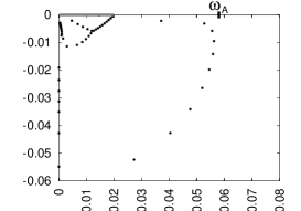
(a) $\gamma=\frac{5}{3}$

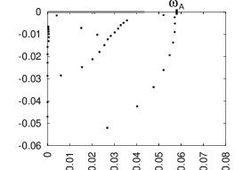
(b) $\gamma=10$

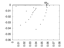
(c) $\gamma=20$

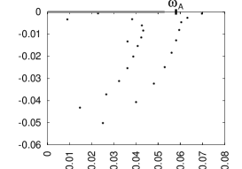
(d) $\gamma=40$

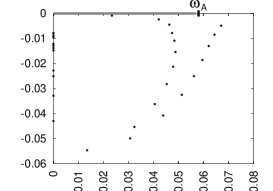
(e) $\gamma=1000$

(f) $\gamma=1000,\rho_{\parallel}\rightarrow 0$

Figure 1: The compressible resistive spectrum of a constant current model ($\beta=4\%$) for various values of $\gamma$. The ideal slow-mode continuum is represented by a grey line on the real axis.

4 Generic spectra in resistive MHD

For general plasma configurations with shear, the resistive Alfvén spectrum is usually found to form a fork (e.g. figure 2 or those in [2] - [5]) The rather different shape of the spectral loci in [figures 1(a)-(f)] is a consequence of the equilibrium having an Alfvén spectrum which degenerates to a point.

Figure 2: A typical eigenvalue spectrum for a compressible ($\gamma=\frac{5}{3}$) resistive MHD case showing the complex frequencies of damped and growing normal modes. In this low-pressure case, slow magnetosonic modes have eigenfrequencies very close to the origin and are not shown. The plasma model parameters are similar to the constant current case, but with a small shear: $m=1$, $\kappa=0.35$, $nq(r)=1.2\times(1-0.1r)$ and $S=3\times 10^{3}$. The ideal Alfvén continuum is represented by a grey line on the real axis.

The fork structure in the resistive MHD spectrum has been qualitatively explained in terms of WKB analysis by examining turning points within the plasma, see [3] and [5]. The fork has three lines joining at a point below the ideal MHD continuum. Two lines run between the intersection point and either end of the Alfvén continuum. The third line runs around approximately in a quarter circle to touch the imaginary axis. In a simple model with toroidal current density constant across the plasma, there is an analytical solution for the $\gamma\rightarrow\infty$ resistive MHD spectrum [6]. We show that a perturbed variant of this constant current model, in which a slight shear is given to the magnetic field, is still amenable to the manipulations performed in [6]. By introducing shear we produce a model which has a finite width Alfvén continuum, in which we might hope to recover the generic fork structure found in compressible results. We therefore solved this model using WKB analysis to explain the qualitatively different spectrum. In the remainder of this paper we set $\rho_{\perp}=\rho_{\parallel}=\rho$.

5 WKB analysis of a small shear equilibrium in the limit $\gamma\rightarrow\infty$

The model case is derived from [6], which considers a cylindrical plasma with a constant axial field and no shear. This model has been studied earlier in [9],[10]. The equations used for this analysis are those of linearised, resistive, incompressible MHD, with $\gamma\rightarrow\infty$:

$$\rho\mu_{0}\frac{\partial}{\partial t}(\mbox{\boldmath$\nabla\times$}\mathbf{v})=\mbox{\boldmath$\nabla\times$}(\mathbf{B}\mbox{\boldmath$\cdot$}\mbox{\boldmath$\nabla$}\mathbf{b}+\mathbf{b}\mbox{\boldmath$\cdot$}\mbox{\boldmath$\nabla$}\mathbf{B}),$$ (5)

and magnetic field given by Ampére’s law

$$\frac{\partial\mathbf{b}}{\partial t}=\nabla\mbox{\boldmath$\times$}(\mathbf{v}\mbox{\boldmath$\times$}\mathbf{B})-\mbox{\boldmath$\nabla\times$}(\frac{\eta}{\mu_{0}}\mbox{\boldmath$\nabla\times$}\mathbf{b}).$$ (6)

The curl of the equation of motion is taken in order to suppress the perturbed pressure. Also, we specialise to an equilibrium state with no plasma velocity.

Figure 3: One period of the cylindrical model.

The idea is to introduce the shear as a small quantity, of the same order as the inverse wave number. The analysis is then the same as the shear-free case, up to two orders in the inverse wavenumber. The radial dependence is included in the dispersion relation in the radially varying quantities: $B_{z}(r)$, $B_{\mathrm{p}}(r)$ and $q(r)$. We first take the large wavenumber limit by ordering $\nabla\simeq O(1/\epsilon)$. For significantly dissipative modes, maximal balance of Ampére’s law (6) occurs for $\epsilon\simeq O(S^{-1/2})$. In a typical physical situation we might have $S>1000$ and thus $\epsilon<0.03$ is a good expansion parameter.

The magnetic field is expressed as $\mathbf{B}=\hat{z}B_{z}(r)+r\hat{\theta}B_{\mathrm{p}}(r)$ with $d(\mbox{log}[B_{\mathrm{p}}(r)])/dr$ and $d(\mbox{log}[B_{z}(r)])/dr$ both of $O(\epsilon)$, in order to satisfy the requirement of small shear. We again look at perturbations of the form $\mathbf{b}=\exp\left(im\theta-i\kappa z/r_{p}-i\omega t\right)\mathbf{b}\left(r\right)$ . For convenience we set $\mathbf{b}$ as $O(1)$ and this then implies $\mathbf{v}$ to be of $O(1)$ to complete the ordering. By using the relations $\nabla\cdot\mathbf{b}=\nabla\cdot\mathbf{v}=0$, equations (5) and (6) can be reduced to:

$$\rho\mu_{0}\frac{\omega}{\tau_{A}}(\nabla\times\mathbf{v})=\frac{B_{p}(r)}{r_{p}}[m-nq(r)]\nabla\times\mathbf{b}+\frac{2B_{p}(r)}{r_{p}^{2}}\kappa\mathbf{b}+O(\epsilon)$$ (7)

and

$$-\frac{i\omega}{\tau_{A}}\mathbf{b}=\frac{iB_{p}(r)}{r_{p}}[m-nq(r)]\mathbf{v}-\frac{\eta}{\mu_{0}}(\nabla\times\nabla\times\mathbf{b})+O(\epsilon).$$ (8)

The safety factor $q(r)$ is given by ${r_{p}B_{z}(r)}/{RB_{p}(r)}$ and the non-dimensional resistivity $\eta=S^{-1}$.

In this form, the only differential operator is the curl operator. This motivates us to look for solutions which are eigenfunctions of this operator, suggesting the ansatz

$$r_{p}\nabla\times\mathbf{v}=\alpha\mathbf{v},\quad r_{p}\nabla\times\mathbf{b}=\alpha\mathbf{b},$$ (9)

which solves equations (7) and (8) provided

$$\alpha(r,\omega)=\frac{2[m-nq(r)]\kappa}{\frac{B_{z}(r)^{2}}{B_{p}(r)^{2}}i\omega[i\omega-S^{-1}\alpha(r,\omega)^{2}]+[m-nq(r)]^{2}}.$$ (10)

By taking the curl of equation (9) we get

$$\nabla\times\nabla\times\mathbf{v}=-\nabla^{2}\mathbf{v}=\frac{\alpha^{2}}{r_{p}^{2}}\mathbf{v},$$ (11)

since the velocity is divergence-free. This implies a relation for the $z$ component of $\mathbf{v}$

$$\frac{1}{r}\frac{d}{dr}r\frac{d}{dr}v_{z}=-\left(\frac{\alpha^{2}}{r_{p}^{2}}+n^{2}-\frac{m^{2}}{r^{2}}\right)v_{z}.$$ (12)

This is amenable to standard WKB analysis if $\alpha$ is large, and in this WKB limit equation (12) is equivalent to:

$$\frac{d^{2}}{dr^{2}}\mathbf{v}_{z}=-Q(r)\mathbf{v}_{z},$$ (13)

with $Q(r)={\alpha^{2}}/{r_{p}^{2}}$. This will break down near the origin ($r=0$) where we will use a Bessel function matching. Equation (13) is solved approximately by:

$$\mathbf{v}_{z}\simeq a_{\mbox{out}}Q^{-\frac{1}{4}}e^{i\phi}+a_{\mbox{in}}Q^{-\frac{1}{4}}e^{-i\phi}$$ (14)

where the amplitudes $a_{\mbox{out}}$ and $a_{\mbox{in}}$ are slowly varying functions, and

$$\phi(r|c)=\int_{c}^{r}Q^{\frac{1}{2}}(r^{\prime})dr^{\prime}$$ (15)

Thus $\alpha/r_{p}$ is the radial wavenumber and equation (10) provides the dispersion relation.

6 Characterising the Stokes points

To find the WKB solutions, it is first necessary to examine the structure of the dispersion relation in the plasma region. In particular, singularities and zeros and the associated branch structure of the dispersion relation must be examined. Branch points of the dispersion relation are known as Stokes points. The dispersion relation (10) can be written as a cubic equation in $\alpha$, with the coefficients as functions of $q(r)={r_{p}B_{z}(r)}/{RB_{p}(r)}$, i.e.

$$\alpha^{3}\frac{1}{S}{\left(\frac{q(r)R}{r_{p}}\right)}^{2}+\alpha{\left([m-nq(r)]^{2}-{\left(\frac{qR}{r_{p}}\right)}^{2}\omega^{2}\right)}=2[m-nq(r)]\kappa.$$ (16)

We would like to discover the singularity structure of our dispersion relation. Solving equation (16) for $\alpha$ leads to very ungainly equations and proves not to be enlightening, so we look for a simpler relation which will be topologically equivalent. Let us consider the case where there is no magnetic surface resonant with the perturbation. In this case we have $[nq(r)-m]\neq 0$ within the plasma, and assuming also $q(r)\neq 0$ then we can divide through the equation by $2[m-nq(r)]\kappa$ and introduce a new variable $\bar{\alpha}$ so that

$${\bar{\alpha}}^{3}+x(r)\bar{\alpha}=1,$$ (17)

with

$$\bar{\alpha}\equiv\alpha\frac{\{2[nq(r)-m]\kappa S\}^{\frac{1}{3}}}{{\left({q(r)R}/{r_{p}}\right)}^{\frac{2}{3}}}$$ (18)

and

$$x(r)\equiv\frac{\left\{[nq(r)-m]^{2}-\left[{qR}/{r_{p}}\right]^{2}\omega^{2}\right\}}{{\left\{2[nq(r)-m]\kappa S{\left({qR}/{r_{p}}\right)}\right\}}^{\frac{2}{3}}}.$$ (19)

The solution of equation (17) for $\bar{\alpha}$ is

$$\bar{\alpha}=-\xi\frac{2^{\frac{1}{3}}\,x}{{\left(27+{\sqrt{729+108\,x^{3}}}\right)}^{\frac{1}{3}}}+\xi^{*}\frac{{\left(27+{\sqrt{729+108\,x^{3}}}\right)}^{\frac{1}{3}}}{3\,2^{\frac{1}{3}}},$$ (20)

where $\xi$ is one of the cube roots of $-1$:

$$\xi=-1, \frac{1+i\,{\sqrt{3}}}{2}, \frac{1-i\,{\sqrt{3}}}{2}.$$ (21)

We consider $x$ as a new radial variable. The function $\bar{\alpha}$ is represented graphically by the Polya plot in figure 4.

Figure 4: One branch of the multivalued function $\bar{\alpha}(x)$ ($\xi=-1$) shown on the complex plane as a Polya plot. Branch cuts are indicated as thick lines. The vector ($\mbox{Re}[\bar{\alpha}],-\mbox{Im}[\bar{\alpha}])$ is displayed on a grid.

By inspection of the form of equation (20) we have candidates for branch points at the three roots of $x^{3}=-27/4$. However, not all of these candidate branch points are true branch points, as suggested by figure 4. This can be seen in the $\xi=-1$ case, where we have, from equation (17)

$$x(\bar{\alpha})=\frac{1-{\bar{\alpha}}^{3}}{\bar{\alpha}},$$ (22)

which can be considered as a local inverse of equation (20).

Let us consider the neighbourhood of $x=-\sqrt[3]{{27}/{4}}$ (using the principal value, so $x$ is a negative real). We might expect a branch point here from the structure of equation (20). At $x=-\sqrt[3]{27/4}$ we have $\bar{\alpha}=2^{2/3}$. However, there is a neighbourhood around $\bar{\alpha}=2^{2/3}$ where equation (22) is analytic and has a non-zero derivative, and therefore the function has an analytic inverse around $x=-\sqrt[3]{27/4}$. There obviously cannot be a branch point in an analytic region. The other two candidate points are true branch points. It similarly follows that each of the other cases of equation (20) have only two branch points each. Note that around a Stokes point at some position $x_{0}$, we do not have $\alpha\propto\sqrt{x-x_{0}}$, as is typical for many WKB analyses [11]. Instead, we have $\alpha\simeq C+D\sqrt{x-x_{0}}$.

7 Phase matching: a solution near the singularities

In order in proceed with WKB analysis, we need to determine the behaviour of solutions near the Stokes points, the branch points of the dispersion relation. In the neighbourhood of the branch point, we approximate the dispersion relation by:

$$Q(x)\simeq 1+Ax^{\frac{1}{2}}.$$ (23)

This is unlike the more usual situation in WKB analysis where $Q(x)\simeq x$ around the Stokes points. The simplest treatment of the phase matching follows from considering $A\ll 1$ in which case the $A=0$ case can be used as a zeroth order solution in a region around the Stokes point. Note that for $A=0$, the dispersion relation is independent of $x$ and there is no reflection of the wave. As we will see, as $A\rightarrow 0$ the reflectivity goes to zero. The transmitted part of the wave will be decaying for finite $A$, so that we have partial absorption of the travelling wave.

Our wave equation is

$$\frac{d^{2}y}{dx^{2}}=-(1+Ax^{\frac{1}{2}})y,$$ (24)

with an $A=0$ solution

$$y_{0}=e^{\pm ix},$$ (25)

which motivates the substitution

$$y=e^{-ix+u(x)}.$$ (26)

The other choice of sign leads to a second solution to the equation, which is growing for $x\rightarrow-\infty$. Substitution of equation (26) into equation (24) leads to

$$A\sqrt{x}-2i\frac{du}{dx}+\left(\frac{du}{dx}\right)^{2}+\frac{d^{2}u}{dx^{2}}=0.$$ (27)

We are looking for small departures from the $A=0$ solutions and in this case we can choose ${du}/{dx}\ll 1$ so that to first order

$$A\sqrt{x}-2i\frac{du}{dx}+\frac{d^{2}u}{dx^{2}}=0,$$ (28)

from which we can find $u^{\prime}(x)$

$${{u^{\prime}(x)}={e^{2\,i\,x}\,C-\frac{i}{8}\,A\,\left[4\,{\sqrt{x}}+\,e^{(2\,x-\pi/4)i}\,{\sqrt{2\,\pi}}\,\mbox{erf}\left(\,e^{-3\pi i/4}{\sqrt{2x}}\right)\right]}}.$$ (29)

The coefficient of integration, $C$, must now be chosen such that we can match the solution on the left-hand side of the origin to the evanescent WKB solution. We have required $u^{\prime}(x)\ll 1$, so an oscillatory $u(x)$ can be modelled as $\epsilon e^{2ix}$ with $\epsilon\ll 1$ (plus a constant which can be safely ignored) in which case:

$$y(x)=e^{-ix+u(x)}=e^{-ix}e^{\epsilon e^{2ix}}\simeq e^{-ix}\left(1+\epsilon e^{2ix}\right)=e^{-ix}+\epsilon e^{ix}.$$ (30)

These correspond to the WKB solutions, which are approximately of the form $c_{1}e^{-ix}+c_{2}e^{ix}$ near the origin. We require that the WKB solution matched on the left-hand side have $c_{2}=0$ because the corresponding term grows exponentially for large negative $x$. We therefore must have $\epsilon\rightarrow 0$ as $x\rightarrow-\infty$. Using the asymptotic expansion of $\mbox{erfc}=1-\mbox{erf}$, as given by equation 7.1.23 of [12], we find the $x\rightarrow-\infty$ limit of equation (29), allowing us to express this matching condition as:

$$C=\frac{A}{8}(1+i)\sqrt{\pi}.$$ (31)

Then we have a solution for $y$ which is asymptotically of the form:

$$y=P(x)\left(e^{-ix}+e^{ix}\frac{A\sqrt{\pi}(1-i)}{4}\right)$$ (32)

for $x\gg 1$, with $P(x)$ a slowly varying function. The phase matching condition is given by finding the nodes of these waves, which fixes the WKB phase at $x=0$:

$$\phi_{0}=\frac{-i}{4}\,\log(\frac{(1+i)A\sqrt{\pi}}{8}).$$ (33)

8 Finding wavemodes

Global modes are found in the usual way: we look for paths $C$ in the complex plane joining the axis and boundary where $\int_{B}\alpha(x)dx$ is real for any sub-path $B$ of $C$. These paths will be WKB solutions if the integral $\int_{C}\alpha(x)dx=\int_{[0,1]}\alpha(x)dx$ which can be guaranteed if there are no singularities of our differential equation coefficients in the region. In particular, this requires that the circular path $C-[0,1]$ does not enclose any Stokes points. The quantisation condition is supplied by requiring the correct behaviour at boundaries. At the origin the WKB wavemode must be matched to a Bessel function, and this gives the condition $\phi|_{x=0}=\pi(1/4+m/2)$. At the outer boundary of the plasma, we require $v_{r}=0$ (fixed plasma boundary), which leads to $\phi|_{x=1}=\pi/2$.

Localised modes proceed from the axis or outer boundary of the plasma and propagate along ray trajectories (which will in this case be anti-Stokes lines) to a Stokes point. They are then evanescent past this point, so it must be possible to draw a path connecting the relevant Stokes point to the other boundary without crossing a Stokes line. For Stokes points of the form $Q(x)=a+bx^{\frac{1}{2}}$, which are present in this analysis, we have a complex phase matching criterion. The phase integral between the Stokes point and the boundary is then required to be complex for matching to occur. This means that we cannot follow anti-Stokes lines, along which the phase is real, exactly to join the boundary and the Stokes point. The complex portion of the phase leads to a correction to the path, which must be taken into account.

9 Application of the WKB method to the small shear incompressible case

For explicit studies, we use a small shear test case:

$$B_{p}(r)=\frac{B_{p0}}{1-r\delta}=\frac{\frac{7}{24}}{1-0.1r},$$ (34)

$$B_{z}(r)=1,R=\frac{20}{7},n=10,m=1,r_{p}=1,q(r)=0.12(1-0.1r)$$ (35)

The WKB trajectories in the complex $r$ plane were determined numerically, and several loci found by finding appropriate paths in the plane, as in [3]. The loci can be characterised by the branch of the dispersion relation which they lie on, and whether the corresponding wave modes are fully global modes or have a turning point inside the plasma.

Although there are three branches of the dispersion relation, on one branch it is never possible in practice to form global modes: the rays inevitably escape towards complex infinity. The other two branches then produce the two forks.

The eigenvalues are displayed in figure 5, together with the numerical result from a code based on [8]. The spectrum is qualitatively similar to a fork structure, but also shares the features of the original simple model. Note that the double loci (running parallel to each other in an arc) are still present in this model.

Figure 5: The resistive spectrum from numerical solution of the MHD equations (circles) compared to the WKB result (plus signs). The ideal Alfvén continuum is represented by a grey bar on the real axis. Plasma parameters are given by equation (35) and $S=3\times 10^{4}$.

The nature of the difference between the two branches of the double locus can be seen in equation (9), and the form of the dispersion function for large enough $\alpha$. Here we have two solutions for $\alpha(\omega)$ such that $\alpha_{1}\simeq-\alpha_{0}$, and the two WKB solutions consist of waves of opposite helicity. Finite pressure gradients in this equilibrium result in waves of opposite helicity having slightly different frequencies.

10 Effects of the $\gamma\rightarrow\infty$ approximation

The reason why we see a pair of loci in 1(e), rather than the single locus usually depicted for compressible spectra (e.g. figure 1(a)) is that in this incompressible model (the limit $\gamma\rightarrow\infty$) there are two classes of wavemodes present which can be excited at the Alfvén frequency. In a uniform field these wavemodes are degenerate: they oscillate at the same frequency. However the two frequencies are split when the plasma contains currents perpendicular to the magnetic field (i.e. in non-force-free plasmas). In the compressible model at low $\beta$, these two degrees of freedom correspond to the slow (magnetosonic) and Alfvén wavemodes and the ratio between slow frequencies and Alfvén frequencies is of order $\beta^{1/2}$.

Force-free models are important special cases, in which pairs of loci of eigenvalues coincide. The $\gamma\rightarrow\infty$ approximation will still result in unphysical eigenmodes. We note the paper of Ryu and Grimm [4], which uses this incompressibility assumption to analyse a case with finite pressure gradients where we should see a double locus structure. We nevertheless see a simple fork structure. We believe that the splitting effect is rather small in this case, so that what looks like one fuzzy locus is in fact a double locus.

11 Conclusions

In plasma physics an assumption of incompressibility is often justified because the parallel dynamics of the plasma and the fluid compression across the field are much less important than the forces due to the magnetic field. For example, incompressibility does not generally affect ideal MHD marginal stability (but this does not extend to resistive MHD [13]).

Two incompressible resistive MHD models were compared with the physical compressible model by analysis of their spectra. For the first model, where the ratio of specific heat is taken to infinity, we expect from local analysis to find two types of wavemodes present at the Alfvén frequency. In the second model where we again set $\gamma\rightarrow\infty$, the parallel plasma inertia is set to zero, and we expect only one Alfvénic mode to be present in the spectrum, corresponding to the physical case. Numerical computation of the spectra of a magnetic shear-free plasma confirms that the second model reproduces most of the eigenmodes associated with the Alfvénic model correctly. The first model has twice as many modes present at the Alfvén timescale.

It is noted that in general most of the modes resolved do not correspond to Alfvén modes and have no physical significance. The shape of an incompressible spectrum for a more general model, with shear present, was determined numerically and by WKB analysis. The unusual nature of the local dispersion relation leads to a complex structure of loci. The resulting spectrum included the ‘double locus’ of the zero shear model and also demonstrated the fork structure that is seen generically for stable resistive MHD spectra.

There are many qualitative features of the resistive Alfvén spectrum that can be reproduced by simply setting $\gamma\rightarrow\infty$. Unfortunately, physical wavemodes and frequencies are not well modelled in this approximation. The stable part of the ideal Alfvén spectrum is irreparably mixed with spurious modes in this limit. However, by using an anisotropic mass density tensor, an incompressibility constraint can be introduced while preserving the Alfvén modes.

Acknowledgments

This work has been supported by the Flinders Institute for Science and Technology, the Australian Institute for Nuclear Science and Engineering and the Australian Partnership for Advanced Computing.

References

References

- [1] Borba, D., Reidel, K. S., Kerner, W., Huysmans, G. T. A., Ottaviani, M., and Schmid, P. J., Physics of Plasmas, 1, 3151–3160 (1994).
- [2] Davies, B., Phys. Letters, 100A, 144–148 (1984).
- [3] Dewar, R. L., and Davies, B., Journal of Plasma Physics, 32, 443–461 (1984).
- [4] Ryu, C. M., and Grimm, R. C., Journal of Plasma Physics, 32, 207–237 (1984).
- [5] Kerner, W., Lerbinger, K., and Reidel, K., Physics of Fluids, 29, 2975–2987 (1986).
- [6] Storer, R. G., Plasma Physics, 25, 1279–1282 (1983).
- [7] Freidberg, J. P., Ideal Magnetohydrodynamics, Plenum Press, New York, 1987, 1st edn.
- [8] Kerner, W., Lerbinger, K., Gruber, R., and Tsunematsu, R., Computer Physics Communications, 36, 225–240 (1985).
- [9] Tayler, R. J., Reviews of Modern Physics, 32, 907–913 (1960).
- [10] Breus, S. M., Zh. Tech. Fiz., 30, 1030–1034 (1960).
- [11] Berk, H. L., and Pfirsch, D., Journal of Mathematical Physics, 21, 2054–2066 (1980).
- [12] Abramowitz, M., and Stegun, I. A., Handbook of Mathematical Functions, Dover Publications, New York, 1965, 9th edn.
- [13] Hender, T. C., Carreras, B. A., Cooper, W. A., Holmes, J. A., Diamond, P. H., and Similon, P. L., Physics of Fluids, 27, 1439–1448 (1984).