Passive scalar diffusion as a damped wave

Three-dimensional turbulence simulations are used to show that the turbulent root mean square velocity is an upper bound of the speed of turbulent diffusion. There is a close analogy to magnetic diffusion where the maximum diffusion speed is the speed of light. Mathematically, this is caused by the inclusion of the Faraday displacement current which ensures that causality is obeyed. In turbulent diffusion, a term similar to the displacement current emerges quite naturally when the minimal tau approximation is used. Simulations confirm the presence of such a term and give a quantitative measure of its relative importance.

1 Introduction

Since the seminal paper of Prandtl (1925), turbulent diffusion has always been an important application of turbulence theory. By analogy with the kinetic theory of heat conduction, the turbulent exchange of fluid elements leads to an enhanced flux, $\overline{\mbox{\boldmath${\mathcal{F}}$}}{}$, of a passive scalar concentration that is proportional to the negative mean concentration gradient,

$$\overline{\mbox{\boldmath${\mathcal{F}}$}}{}=-\kappa_{\rm t}\mbox{\boldmath$\nabla$}{}\overline{C}\quad\mbox{(Fickian diffusion)},$$ (1)

where $\kappa_{\rm t}={1\over 3}u_{\rm rms}\ell_{\rm cor}$ is a turbulent diffusion coefficient, $u_{\rm rms}$ is the turbulent rms velocity, and $\ell_{\rm cor}$ is the correlation length. Equation (1) leads to a closed equation for the evolution of the mean concentration, $\overline{C}$,

$${\partial\overline{C}\over\partial t}=\kappa_{\rm t}\nabla^{2}\overline{C}.$$ (2)

This is an elliptic equation, which implies that signal propagation is instantaneous and hence causality violating. For example, if the initial $\overline{C}$ profile is a $\delta$-function, it will be a gaussian at the next instant, but gaussians have already infinite support.

The above formalism usually emerges when one considers the microphysics of the turbulent flux in the form $\overline{\mbox{\boldmath${\mathcal{F}}$}}{}=\overline{\mbox{\boldmath$u$}{}\int\dot{c}\,{\rm d}t}$, where $\dot{c}\approx-\mbox{\boldmath$u$}{}\cdot\mbox{\boldmath$\nabla$}{}\overline{C}$ is the linear approximation to the evolution equation for the fluctuating component of the concentration. Recently, Blackman & Field (2003) proposed that one should instead consider the expression

$$\partial\overline{\mbox{\boldmath${\mathcal{F}}$}}{}/\partial t=\overline{\dot{\mbox{\boldmath$u$}{}}c}+\overline{\mbox{\boldmath$u$}{}\dot{c}}.$$ (3)

On the right hand side, the nonlinear terms in the two evolution equations for $u$ and $c$ are not omitted; they lead to triple correlations which are assumed to be proportional to $-\overline{\mbox{\boldmath${\mathcal{F}}$}}{}/\tau$, where $\tau$ is some relaxation time. Furthermore, there is a priori no reason to omit the time derivative on the left hand side of equation (3). It is this term which leads to the emergence of an extra time derivative (i.e. a ‘turbulent displacement flux’) in the modified ‘non-Fickian’ diffusion law,

$$\overline{\mbox{\boldmath${\mathcal{F}}$}}{}=-\kappa_{\rm t}\mbox{\boldmath$\nabla$}{}\overline{C}-\tau{\partial\overline{\mbox{\boldmath${\mathcal{F}}$}}{}\over\partial t}\quad\mbox{(non-Fickian)}.$$ (4)

This turns the elliptic equation (2) into a damped wave equation,

$${\partial^{2}\overline{C}\over\partial t^{2}}+{1\over\tau}{\partial\overline{C}\over\partial t}={\textstyle{1\over 3}}u_{\rm rms}^{2}\nabla^{2}\overline{C}.$$ (5)

The maximum wave speed is obviously $u_{\rm rms}/\sqrt{3}$. Note also that, after multiplication with $\tau$, the coefficient on the right hand side becomes ${\textstyle{1\over 3}}\tau u_{\rm rms}^{2}=\kappa_{\rm t}$, and the second time derivative on the left hand side becomes unimportant in the limit $\tau\to 0$, or when the physical time scales are long compared with $\tau$.

2 Validity of turbulent displacement flux and value of $\tau$

A particularly obvious way of demonstrating the presence of the second time derivative is by considering a numerical experiment where $\overline{C}=0$ initially. Equation (2) would predict that then $\overline{C}=0$ at all times. But, according to the alternative formulation (5), this need not be true if initially $\partial\overline{C}/\partial t\neq 0$. In practice, this can be achieved by arranging the initial fluctuations of $c$ such that they correlate with $u_{z}$. Of course, such highly correlated arrangement will soon disappear and hence there will be no turbulent flux in the long time limit. Nevertheless, at early times, $\langle\overline{C}^{2}\rangle^{1/2}$ (a measure of the passive scalar amplitude) rises from zero to a finite value; see Fig. 1.

Figure 1: Passive scalar amplitude, $\langle\overline{C}^{2}\rangle^{1/2}$, versus time (normalized by $u_{\rm rms}k_{\rm f}$) for two different values of $k_{\rm f}/k_{1}$. The simulations have $256^{3}$ meshpoints. The results are compared with solutions to the non-Fickian diffusion model.

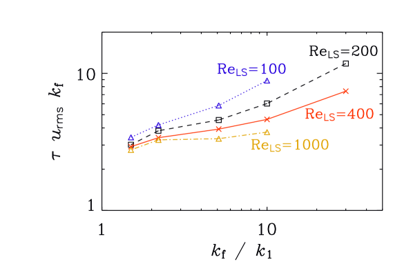
Figure 2: Strouhal number as a function of $k_{\rm f}/k_{1}$ for different values of $\mbox{Re}_{\rm LS}$, i.e. the large scale Reynolds number. The resolution varies between $64^{3}$ meshpoints ($\mbox{Re}_{\rm LS}=100$) and $512^{3}$ meshpoints ($\mbox{Re}_{\rm LS}=1000$).

Closer inspection of Fig. 1 reveals that when the wavenumber of the forcing is sufficiently small (i.e. the size of the turbulent eddies is comparable to the box size), $\langle\overline{C}^{2}\rangle^{1/2}$ approaches zero in an oscillatory fashion. This remarkable result can only be explained by the presence of the second time derivative term giving rise to wave-like behavior. This shows that the presence of the new term is actually justified. Comparison with model calculations shows that the non-dimensional measure of $\tau$, $\mbox{St}\equiv\tau u_{\rm rms}k_{\rm f}$, must be around 3. (In mean-field theory this number is usually called Strouhal number.) This rules out the validity of the quasilinear (first order smoothing) approximation which would only be valid for $\mbox{St}\to 0$.

Next, we consider an experiment to establish directly the value of St. We do this by imposing a passive scalar gradient, which leads to a steady state, and measuring the resulting turbulent passive scalar flux. By comparing double and triple moments we can measure St quite accurately without invoking a fitting procedure as in the previous experiment. The result is shown in Fig. 2 and confirms that $\mbox{St}\approx 3$ in the limit of small forcing wavenumber, $k_{\rm f}$. The details can be found in Brandenburg et al. (2004). A Visualization of $C$ on the periphery of the simulation domain is shown in Fig. 3 for $k_{\rm f}=1.5$. Note the combination of large patches (scale $\sim 1/k_{\rm f}$) together with thin filamentary structures.

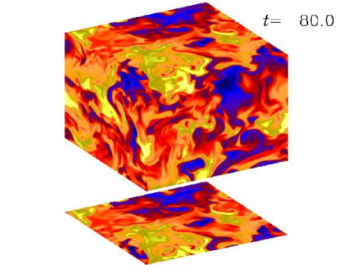
Figure 3: Visualizations of $C$ on the periphery of the simulation domain at a time when the simulation has reached a statistically steady state. $k_{\rm f}/k_{1}=1.5$, $\mbox{Re}_{\rm LS}=400$.

Finally, we should note that equation (3) in the passive scalar problem was originally motivated by a corresponding expression for the electromotive force in dynamo theory, where the $\dot{\mbox{\boldmath$u$}{}}$ terms leads to the crucial nonlinearity of the $\alpha$-effect (Blackman & Field 2002).

References

- (1) Blackman, EG, Field, GB (2002) New dynamical mean-field dynamo theory and closure approach. Phys. Rev. Lett. 89:265007
- (2) Blackman, EG, Field, GB (2003) A simple mean field approach to turbulent transport. Phys. Fluids 15:L73–L76
- (3) Brandenburg, A, Käpylä, P, & Mohammed, A (2004) Non-Fickian diffusion and tau-approximation from numerical turbulence. Phys. Fluids 16:1020–1027
- (4) Prandtl, L (1925) Bericht über Untersuchungen zur ausgebildeten Turbulenz. Zeitschr. Angewandt. Math. Mech.. 5:136–139