Quantum Monte Carlo Studies of Superfluid Fermi Gases
Abstract
We report results of quantum Monte Carlo calculations of the ground state of dilute Fermi gases with attractive short range two-body interactions. The strength of the interaction is varied to study different pairing regimes which are characterized by the product of the -wave scattering length and the Fermi wave vector, . We report results for the ground state energy, the pairing gap and the quasiparticle spectrum. In the weak coupling regime, , we obtain BCS superfluid and the energy gap is much smaller than the Fermi gas energy . When , the interaction is strong enough to form bound molecules with energy . For we find that weakly interacting composite bosons are formed in the superfluid gas with and gas energy per particle approaching . In this region we seem to have Bose-Einstein condensation (BEC) of molecules. The behavior of the energy and the gap in the BCS to BEC transition region, is discussed.
pacs:
03.75.Ss, 05.30.Fk, 21.65.+fI INTRODUCTION
How pairing evolves from the bare interaction has been a major question in condensed matter physics, and the study of pairing in relation to the phenomenon of superfluidity and superconductivity can be traced back to Cooper et al. cooper (1959). Pairing lies at the core of several quantum many-body problems, and it is also believed to influence the evolution of neutron stars Pethick and Ravenhall (1995). Here we report results of quantum Monte Carlo calculations of a superfluid Fermi gas with short range two-body interactions. The strength of the interaction is varied to study different regimes of pairing.
The evolution of pairing with the strength of the interaction has been discussed in the literature Leggett (1980), Randeria (1995). In the regime where the interaction is weak and attractive, a gas of fermions has a superconducting instability at low temperatures, and a gas of Cooper pairs is formed. The typical coherence length is larger than the interparticle spacing ( with the number density) and the bound pairs overlap. In contrast, in the strong-coupling limit the coherence length is small, and the bound pairs can be treated as well seperated Bose molecules. One then expects the molecules to undergo Bose-Einstein condensation (BEC) into a single quantum state with zero momentum.
The Bardeen-Cooper-Schrieffer(BCS) theory Leggett (1980) and Gorkov equations Gorkov and Melik-Barkhudarov (1961) have been used to estimate gaps in superfluid gases. However, their predictions differ by more than a factor of two and they may be qualitatively valid only in the weakly interacting regime. Here we use first principle quantum Monte Carlo methods to study the entire region ranging from free fermions to the tightly bound Bose molecules.
Dilute Fermi gases of 40K, 6Li, 2H for example, can now be studied in the laboratory using magnetic and optical trapping and ingenious cooling methods De Marco et al. (1999), O’Hara et al. (2002). These are dilute Fermi systems, in contrast to dense atomic liquid 3He or a solution of 3He in superfluid 4He. Within the last few years temperatures have been achieved, where is the Fermi kinetic energy and is the Fermi wave vector. At such a low temperature, the fermionic nature of the quantum statistics becomes evident in the measurement of the density profile of the trapped gas. At even lower temperatures the transition to the superfluid Cooper-paired state is expected. However, the temperature of this transition can be much lower than and conclusive evidence of superfluidity is still to be seen. In order to have the transition at an achievable temperature, the experimentalists rely on the Feshbach resonance technique to produce strong interaction between the fermionic atoms.
When the range of the interatomic interaction is smaller than all the length scales in the system, the details of the interaction are believed to be unnecessary and the scattering length is sufficient to characterize it. Near the resonance, the magnitude of the scattering length becomes much larger than and the system enters the strong-coupling regime. The value has been achieved by O’Hara et al. O’Hara et al. (2002) and the limit () is now approached in the laboratory Stenger et al. (1999), Roberts et al. (2001). Recently, creation of bosonic molecules from 40K atoms was reported by Regal et al. Regal et al. (2003), and pairing in the regime was observed (Ref. Regal et al. (2004)).
A few words are in order regarding the language of -wave scattering. For a noninteracting system at zero temperature, the only length scale is . We can use the dimensionless quantity to describe a dilute gas having interparticle spacing much greater than the interaction range. We often use because changes discontinuously from to when a bound state is formed at . For attractive interactions can change from large negative values (weakly interacting limit) to large positive values (strongly interacting limit). As discussed in section II, the radius of the bound molecule provides another length scale in the strongly interacting regime. Some physical examples of the limits of are: 1) electrons in superconductors have large and negative; 2) neutron matter has small and negative; and 3) cold deuterium atoms have large positive . In the last case, molecular bound states smaller than the average interparticle distance are possible. On the other hand, superfluid 3He is not describable in terms of , because the interaction range is greater than , and the paired state does not have -wave symmetry.
In the limit of zero energy for the colliding pair, the two-body scattering cross section is given by . When , the interatomic collisions in the gas are similar to those in vacuum, and the mean free path is approximately given by . However, this approximation is meaningful only when and . When is the two-body collisions in the gas are strongly influenced by the presence of other particles, and their cross section in the gas is much smaller than in vacuum.
For a Fermi gas at low density, an expansion of the energy in terms of is possible. For spin Fermi gases it is known to be Lenz (1929), Huang (1957)
| (1) |
where is the ground state energy per particle of the noninteracting Fermi gas. In the limit, theoretical estimates of 0.326 and 0.568 were reported Baker (1999), Heiselberg (2001). More recently, the authors Carlson et al. (2003) predicted using quantum Monte Carlo methods. In this paper we continue that study of the properties of cold dilute spin fermion gas and extend it to all the regimes of as a first step for understanding the superfluidity and the bosonization of dilute Fermi gases.
The model considered in this study consists of fermions contained in a box with periodic conditions on its boundaries. It is not polarized so that half of the spins point up and the other half down. Typically is varied from 10 to 20 to estimate properties of uniform gas in the thermodynamic limit. In some cases larger values of are used. Fermions of the same spin do not feel the effects of interaction because it is of short range and Pauli exclusion predominates. The fermions of different spins interact via a central potential with the following properties: 1) It is attractive with very short range as we assume the dilute limit, 2) The details of the potential do not matter, in principle we can think of it as an attractive delta function potential, and 3) The potential can be adjusted such that we can sweep through different regimes of .
From the considerations mentioned above, a potential of the form
| (2) |
can be used. The strength of potential () is adjusted to obtain the desired value of . We can also take appropriate values of such that the effective range of the potential is much smaller than the interparticle distance . When this potential has and . In most calculations we have used . For the case we also tested the limit using Carlson et al. (2003).
Results of simple lowest order constraint variational (LOCV) calculations are reported in section II. The LOCV method was first used to study neutron matter Pandharipande et al. (1973). Recently, Cowell et al. Cowell et al. (2002) have used it to study cold Bose gases in the unstable regime. It provides a surprisingly good estimate of the ground state energy. Here we use it to study the effect of the difference between the () and delta-function potentials on the energy of dilute gases. The difference becomes significant when , and the radius of the molecule approaches . LOCV is also used to estimate the energy of the unstable state of the Fermi gas for . The stability of dilute gases is discussed in the LOCV section II.
One of the limitations of LOCV is that it can not be used to calculate the pairing energy gap or the other superfluid properties of Fermi gases. The quantum Monte Carlo methods used in Ref. Carlson et al. (2003) and this work to study superfluid gases are described in section III, and the results for the energy, pairing gap and the quasiparticle spectrum are presented in section IV over the range to to . Conclusions are given in the last section V.
II Lowest Order Constraint Variational CALCULATIONS
In the lowest order constraint variational (LOCV) method the ground state of the Hamiltonian
| (3) |
where the unprimed index denotes spin up particle, primed index denotes spin down particle, and can be any particle, is approximated by the Jastrow-Slater wave function
| (4) |
where is the ground state of noninteracting fermions. In the present case is a product of two Slater determinants, the first corresponding to the spin up fermions and the second corresponding to the spin down fermions. The interaction effects are represented by the Jastrow function , where denotes the pair correlation function. We often use to denote . means no correlation between the pair and for correlated pairs. In variational calculations, the function is determined by minimizing the expectation value of the Hamiltonian
| (5) |
The assumption behind LOCV is that the energy is most sensitive to the correlations of short (less than ) range. We impose a constraint on the range of to assure that the correlations are mostly among the closest pairs, and keep only the pair terms in the cluster expansion of the energy expectation value. The healing distance is the range of defined such that and . In LOCV, is chosen such that on average there is only one other particle within the distance of any particle. Effects of deviations from this average are assumed to cancel.
Euler-Lagrange minimization of the energy expectation valueSchmidt et al. (1977) gives a Schrödinger-like equation for
| (6) |
The constraint used to determine the healing distance is
| (7) |
and the is chosen such that . In the equations (6) and (7) we do not have exchange contributions because the range of the interaction is short and fermions of same spin do not interact. When the equations (6) and (7) are simultaneously solved, the energy per particle is given by
| (8) |
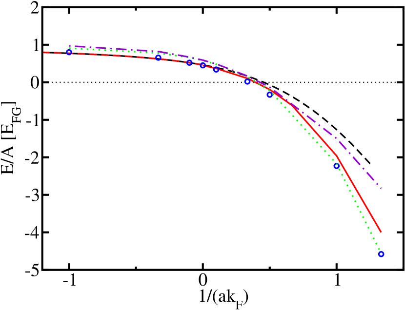
The results obtained for the ground state energy of spin Fermi gas with the and delta-function potentials are shown in Fig. 1.
When the is the only length scale in the gas, and the results obtained with the potential with are indistinguishable from those given by the delta-function potential. In contrast, when , we have a molecular bound state whose radius provides another length scale. At large positive values of there are differences between results of the present and delta-function potentials due to the rms radius, of the molecule becoming comparable to the range of the present potential. For example, at we get with the present choice of . In principle, we can continue to approximate the delta-function interaction with the potential by further increasing , and working in the limit. However, all of the present computations are with .
Fig.1 also shows the presumably exact results obtained with the potential with the GFMC method described in the next section. The LOCV energies appear to be surprisingly accurate. However, it should be realized that a part of the accuracy of LOCV is due to a cancellation of errors, and not due to the quality of the Jastrow-Slater variational wave function (Eq. 4). In fact, the variational energy upper bound obtained with that wave function for is , significantly above GFMC result of . The LOCV energy of is below the Jastrow-Slater variational upper bound because it is calculated approximately keeping only two-body cluster contributions. However, when the contributions of -body clusters become important we can expect that the approximations in the Jastrow-Slater wave function would also become important, and the true energy will be below the Jastrow-Slater upper bound.
The ground state energies obtained with the conventional BCS (variational) method are also shown in Fig. 1. In the weakly interacting limit, , the BCS energy is too large since it does not have the correct low density limit given by Eq. 1. On the other hand, in the strongly interacting limit, , the BCS energy is very close to the exact result (GFMC) presumably because in this limit we have complete pairing of the fermions into Bose molecules. LOCV is less accurate than the conventional BCS method in strong coupling region.
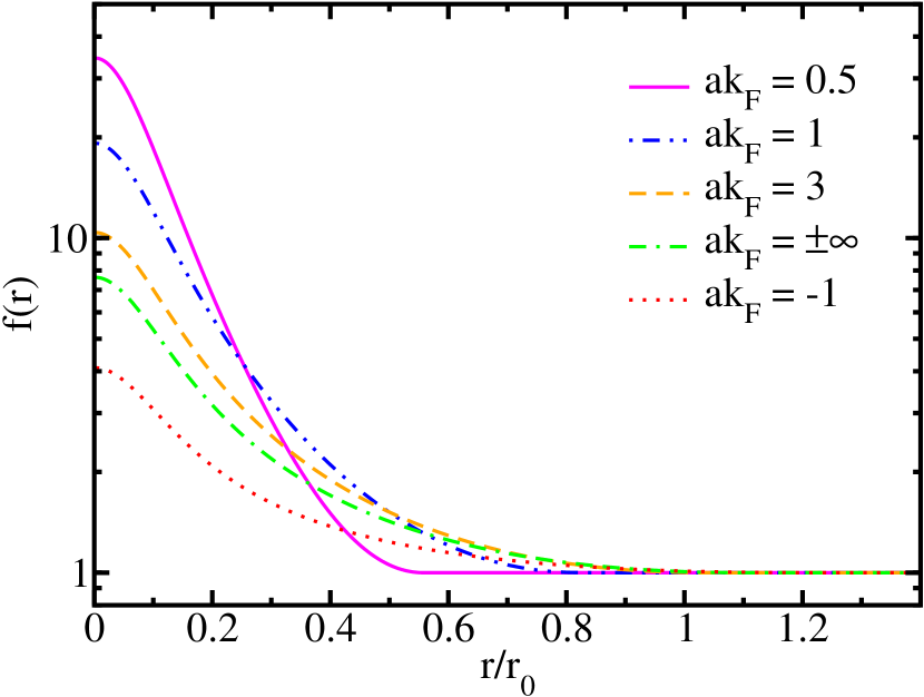
The LOCV pair correlation functions are shown in Fig. 2. The healing distance in the weakly interacting region (), and as we increase the strength of the potential, becomes more and more peaked at the origin, and becomes smaller than . In fact for , the boundary condition at has less impact on and of the Eq. 6 becomes close to the molecular binding energy such that . is the term that predominates in this limit. is small () and negative so that .
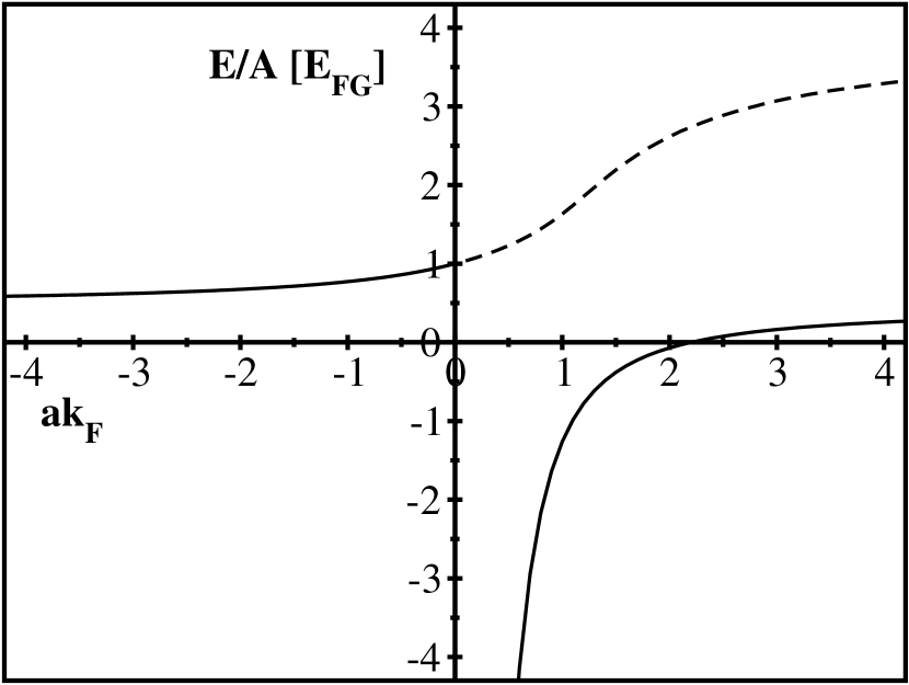
When we can obtain another solution of the LOCV equation with a node at . This solution was discussed by Cowell et al. Cowell et al. (2002) for cold Bose gases, and at small values of it gives results in agreement with the low density expansion, (Eq.1). The first term () is correctly reproduced by LOCV, but the higher order terms are approximate. In the limit we have the condition discussed in Ref. Cowell et al. (2002). The solution with one node is and it gives . Results obtained with the delta-function potential, including this unstable region are shown in Fig. 3. Those corresponding to the nodeless solution of the LOCV equation are represented by full line, while the dashed line corresponds to the solution with a node.
The state of the gas having a node in the pair correlation function is unstable because it has energy , while that with nodeless has lower energy (see Fig. 3). However, it can have a relatively long life time because energy conservation prevents two atoms to make the transition to the lower energy state. At least three atoms are needed, which hinders the transition at low densities. Most of the observed BEC of Bose atoms are in such unstable states in which the has nodes at small .
The shown by the solid line in Fig.3 corresponds to the stable ground state of the model Hamiltonian with the delta-function interaction. In principle, this state can be exactly calculated by the quantum Monte Carlo method described in the next section. However, when the range of the interaction is finite, as for the model, the system can collapse to a tightly bound state at large density. This instability can be easily seen in the Hartree mean field approximation in which
| (9) |
where is the volume integral of the interaction. At large enough the interaction energy becomes larger than leading to a tightly bound state.
Consider for example a simple square well potential of range such that and . Let this potential correspond to . This means and, . Then
| (10) |
The collapse occurs at values of , and can be pushed to higher densities by reducing , or equivalently increasing in the case of the potential. In the present studies, we ignore this collapsed state; assuming that it occurs at too large a density to influence the dilute gas properties.
III Green’s Function Monte Carlo CALCULATIONS
Green’s function Monte Carlo (GFMC) Kalos (1974) is a powerful method for calculating the ground state properties of many-body quantum systems. It can be used to calculate the ground state properties of Bose systems with controllable statistical errors without approximation. For the fermion systems, however, we have to deal with the sign problem posed by the anti-symmetry of the wave function as discussed below. We begin with a brief overview of the GFMC method.
Let be the eigenstates of with eigenvalues . The trial variational wave function , which provides an approximation to the ground state , can be expanded as
| (11) |
In GFMC we project out from by evolution in imaginary time
| (12) | |||||
where we have shifted the origin of energy to to control the norm of . In practice, the time evolution is carried out in small steps
| (13) |
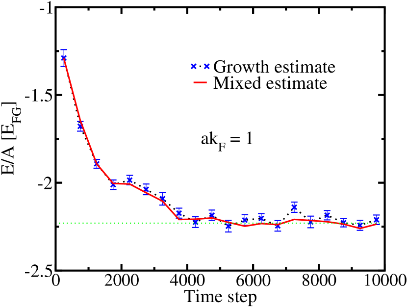
and is tuned to keep constant. The tuned provides the growth estimate of the true . An alternative method for calculating the ground state energy, often with smaller statistical error, is given by the mixed estimate (see Fig. 4)
| (14) |
In general, the time evolution operator or propagator is not known for arbitrary large value of except for few simple systems. However, we can obtain small time propagator with controllable errors for any Hamiltonian with static potentials that depend only on the positions of the particles denoted by a -dimensional configuration vector . This is the motivation to write the time evolution as a product of many short time operators (Eq. 13). We define the Green’s function
| (15) |
The propagation equation becomes
| (16) |
The primitive approximation to this Green’s function is
| (17) |
where and is the Green’s function for free particles
| (18) |
This approximation has errors of order . The total error after time steps is of the order . The corrections to this expression can be sampled to make an exact algorithm. Here we use the more common method and make this error as small as we want, by increasing the number of steps . In practice, this error is made smaller than the statistical sampling errors of the Monte Carlo integration.
A naive quantum Monte Carlo algorithm could start with configuration vectors sampled from . These provide the approximate representation
| (19) |
where or depending on the sign of . The accuracy of this representation increases with the number of samples . Inserting Eq. 19 into Eq. 16 and using the short time approximation, gives as a sum of normalized gaussians times weight factors containing the product of the original and the exponentials in short time Green’s function (Eq. 17). Sampling a position from each of the gaussians gives a representation of as a sum of delta functions times weight factors with signs. This process is repeated times to obtain . During the evolution, large magnitude weight factors are converted into multiple copies while small factors are sampled and kept with unit magnitude new weight with a probability proportional to the magnitude of the old weight. The random walk of the weighted -function samples representing the propagation of , therefore consists of diffusing and branching and the number of samples at each time step can vary.
This algorithm suffers from the fermion sign problem. For samples , , and weights , the denominator of a matrix element such as the mixed energy will be the sum . Each carries the sign of the initial sample from , and if the path of the sample has crossed nodes of odd number of times, the contribution to the sum will be negative. For large times the contribution of these negative paths almost completely cancel the contribution of positive paths that have not crossed nodes or crossed an even number of times. The signal dies out exponentially compared to the statistical noise. The numerator suffers from the same problem.
The fixed nodeAnderson (1975) approximation deals with the fermion sign problem by restricting the path so that crossings of the nodal surface are not allowed. When this constraint is imposed with the nodal surface of the exact fermion ground state, converges to that state. Imposing the nodal surface from an antisymmetric trial function gives an upper bound
| (20) |
We impose the fixed-node constraint with the nodes of our trial function .
Importance sampling is used to control the fluctuations of the weights. The propagation equation is modified by multiplying by a positive importance function. Since we are using the fixed node approximation, the paths have zero probability of crossing the nodes, and we can take the importance function to be the absolute value of . The propagation equation now becomes
| (21) |
The short time approximation for the importance sampled Green’s function is
| (22) | |||||
where the local energy is
| (23) |
Since is still a normalized gaussian, the only changes to the naive algorithm are the sampling of the drifted Gaussian, and the new weight given by the terms in the braces. Notice that if is close to the ground state of , will have less fluctuations than , and the branching of the walk is much reduced. Any paths that cross a node due to the short time approximation are eliminated.
For samples , all with weight , at time , the mixed energy becomes the average of the local energy
| (24) |
Since the fixed node calculations give an upper bound to the ground state energy, our strategy (see Ref. Carlson et al. (2003)) is to choose a trial wave function with variable nodal surfaces and minimize the fixed node GFMC .
The trial wave function is now used in three different contexts; 1) as the initial guess of the ground state, 2) as the importance function in Eq. 21, and 3) as the node restriction function. The nodes of the Jastrow-Slater wave function (Eq. 4) equal those of noninteracting Fermi gas and can not be varied. So that wave function is not useful for present studies.
From physical considerations, a better trial wave function must reflect the fact that the fermions with attractive interaction can form bound Cooper pairs in the ground state. And from mathematical considerations, the trial wave function must have variable nodal surface, which can be varied to minimize the fixed node GFMC energy. The BCS wave function is such a wave function. Commonly, we write
| (25) | |||||
where denotes the vacuum and and are real positive numbers. However, this wave function does not correspond to a definite number of particles. In fact, expanding the wave function we can write
| (26) |
where is the pair creation operator. The component that corresponds to particles or pairs can be obtained by transforming
| (27) | |||||
This component can be written as an antisymmetrized product of the pair wave functions
| (28) | |||||
where the number of up spin particles () is equal to the number of down spin particles (). The variational parameters are real positive numbers. The free fermion gas, Slater wave function is just a particular case of this wave function when for and for .
We also consider systems having unpaired particles. In particular, we can have pairs and 1 unpaired up or down spin particle. This generalization is necessary as the gap energy is calculated from the odd-even staggering of the ground state energy Carlson et al. (2003). With 1 unpaired ( or spin) particle in the state , with momentum , the trial wave function is given by Bouchaud et al. (1988)
| (29) |
The ground state is expected to have in the weakly interacting regime and in the strongly interacting regime. This wave function can be calculated as a determinant Bouchaud et al. (1988),Carlson et al. (2003), which makes the numerical calculations relatively simple.
Quantum Monte Carlo calculations use a finite number of particles in a cubic periodic box of volume to simulate the infinite uniform system. The momentum vectors in this box are discrete
| (30) |
and the system has a shell structure with closures occurring when the total number of particles = 2, 14, 38, 54, for spin- fermions. The shell number is defined such that , and .
In the present calculations, the pair wave function has the assumed form
| (31) | |||||
Here is a cut off shell number. We assume that the contributions of shells with to the pair wave function can be approximated by a spherically symmetric function of range . We further reduce the statistical fluctuations by using the Jastrow factor along with in the variational wave function:
| (32) |
The Jastrow factor does not change the nodal structure. Thus, the average value of the estimated energy is independent of , but the statistical error is reduced by using the from LOCV calculations.
It is convenient to require that at . This is because the local energy has terms like which can have large fluctuations at the origin when at . The factor cuts off dependence of at . The energies are not too sensitive to the parameter , and its value is fixed at . In addition, is chosen such that at ; its value is in the limit .
The variational parameters are and . We wish to find a set of these parameters that minimize the fixed node GFMC estimate of energy. However, considering that we have to allow simultaneous variation of all the parameters, methods based on unguided variation become difficult, if not infeasible. Again, we rely on the GFMC procedure itself to optimize these parameters. Initial configurations are obtained with a random distribution of the parameters centered around a reasonable guess. Each of them is propagated according to the nodal constraints provided by their parameters with a single . The paths with the smallest acquire large amplitudes or weights as . The average among these paths gives an optimization over the initial random distribution. This process is repeated several times until convergence is achieved.
When we have an odd number of particles, the ground state momentum (Eq. 29) is an additional variational parameter. We minimize the fixed node GFMC energy of systems with odd by varying . As discussed in the results section, the magnitude of changes from to as the interaction strength increases and we go from the weakly interacting BCS to strongly interacting BEC regime. The gap energy is obtained from the odd-even staggering of the total energy
| (33) |
In doing so, the effects of interaction among quasiparticles are neglected.
IV RESULTS
The values of the parameters, and , of the BCS wave function are to be determined by minimizing the fixed node GFMC mixed energy for each value of and . The minimum energy obtained is our estimate for the ground state energy of the system. The values of the parameters that minimize this energy are not very sensitive to , the number of particles in the box. We find it sufficient to determine the optimum parameters at and , and interpolate their values in the and ranges. The values of the parameters at these values of are listed in Table 1.
At the lowest energies are obtained without any short range and the optimum pair function has contributions only from the states with . This is consistant with the weak coupling BCS theory in which goes to zero when becomes large.
When , lower energies are obtained with . In most cases, the values of the parameters do not change significantly between and . The values listed in Table 1 for are used for .
In the range, the optimum values of the parameters of do not seem to change significantly with the . We have not obtained any significant improvements to the energy from varying the parameters in the region . In this region we retain the values found for and . Recall that only the nodal surfaces of the ground state wave function are constrained by those of . The complete has an additional product of Jastrow pair correlation functions which depends on , and the true ground state wave function changes continuously with .
The magnitude of the momentum of the unpaired particle in the ground state is also determined by minimizing the GFMC fixed node energy. The minimum values are listed in Table 2. In the weak coupling limit, the BCS ground state for odd has . In the periodic box, the value of is 1 for , and 2 for in units of . In the to range, the minimum values of are as indicated by the weak coupling BCS theory. However, in the to range the is 1 for the entire range (11 to 19) of odd values of considered. At the states with and 1 are almost degenerate, and for the ground states of odd systems have , as expected when the system consists of bound molecules condensed in the zero momentum state, and the unpaired particle also in the state.
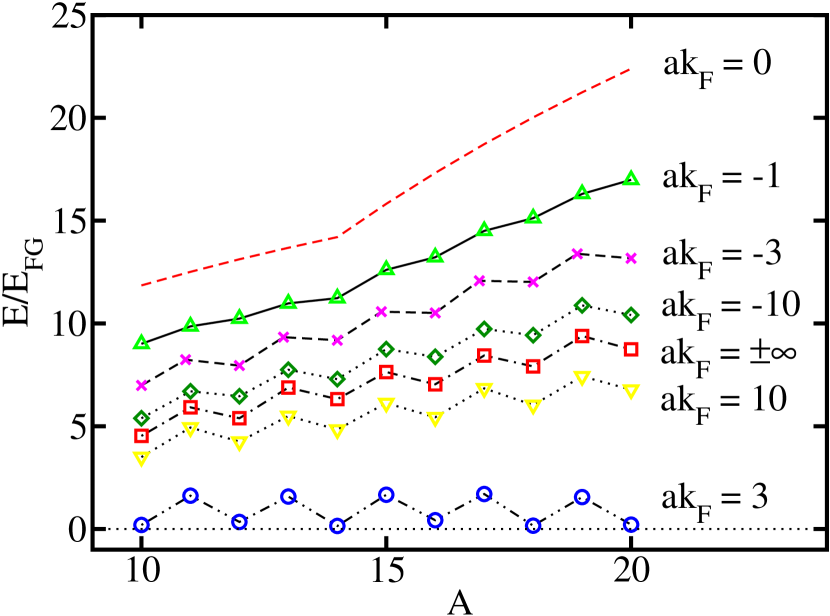
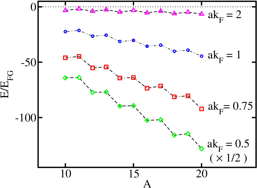
The calculated values of the ground state energy are shown in figures 6 and 7. The systems with seem to have , while those with can have . When the two-body interaction is strong enough to bind two particles and form molecules with energy . The energy per particle, of the superfluid Fermi gas is compared with in figure 8. Within the computational errors (see Table 3), however at we find that is very close to . This behavior also indicates that at these values of the system approaches that composed of Bose molecules forming a BEC. It has been argued that the interaction between these molecules is weakly repulsive, with a molecule-molecule scattering length given by petrov et al. (2003). In this case the will always be greater than , and the gas will have positive pressure, increasing with the gas density or .
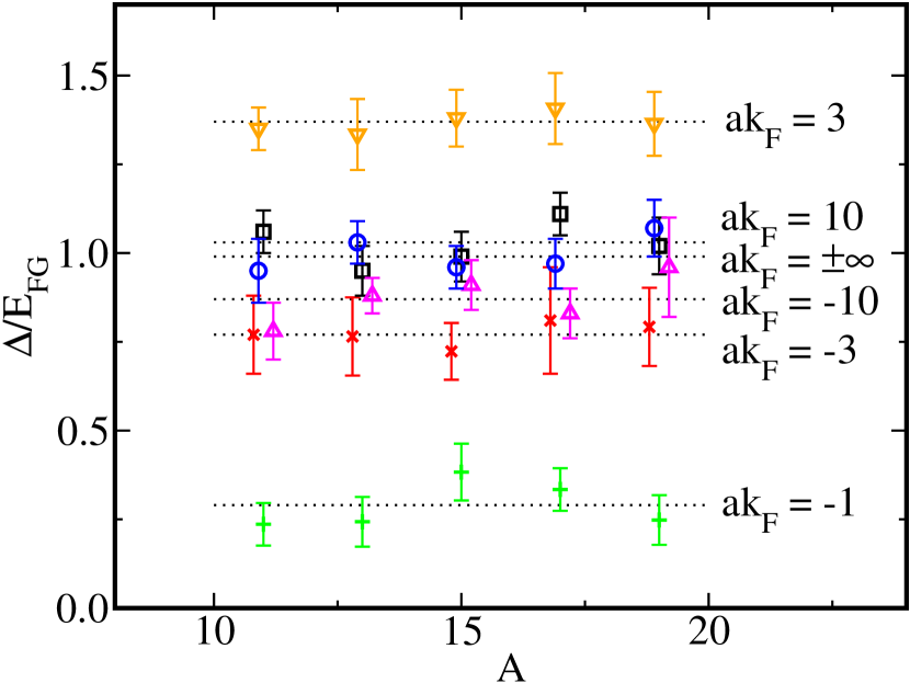
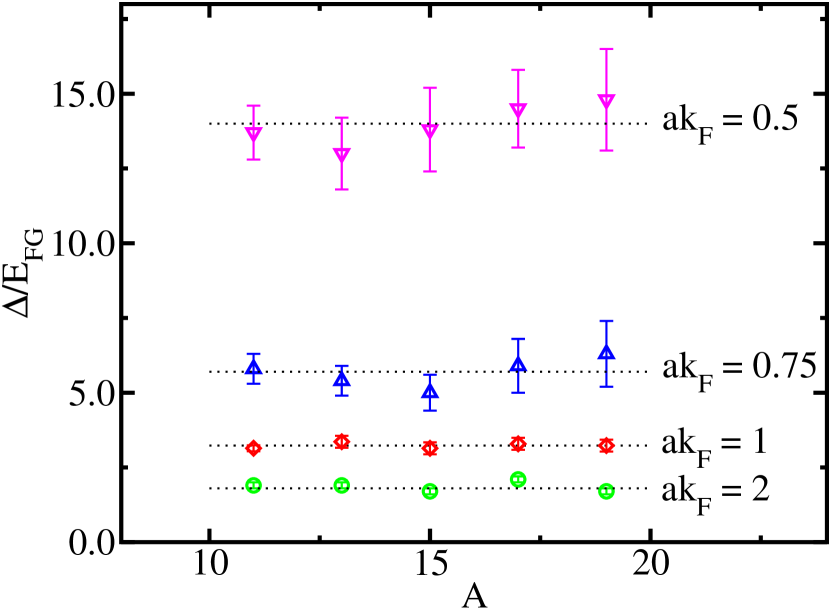
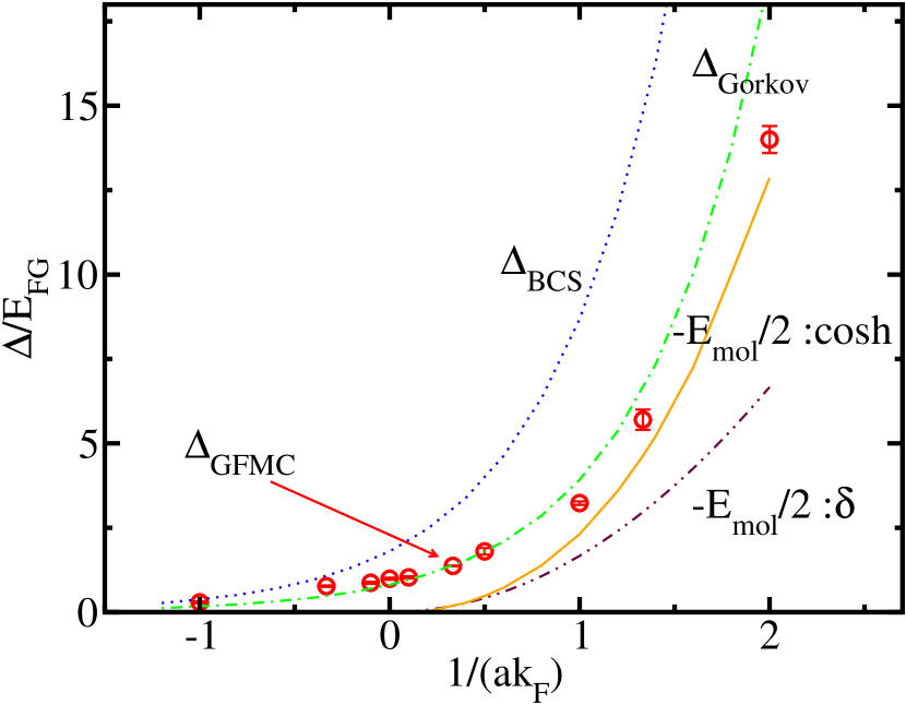
The pairing gaps calculated from the odd-even energy difference (Eq. 33) are shown in figures 9 and 10. These gaps are not very sensitive to , and they are compared with the predictions of BCS Leggett (1980) and Gorkov Gorkov and Melik-Barkhudarov (1961) estimates given by
| (34) |
where the chemical potential is approximated by as when . At the calculated gaps are in between these estimates, while at positive values of they approach as expected for a gas of Bose molecules (see Fig. 10 and Table 3).
Figures 8 and 11 also show the for a delta-function interaction in addition to those for the present potential with . The two potentials give essentially the same results for , but at larger values the potential is more attractive. The values of the radius of the molecule are listed in Table 3. At large values of the is not very large for the present choice of , and much larger values of should be used to approximate the delta-function interaction.
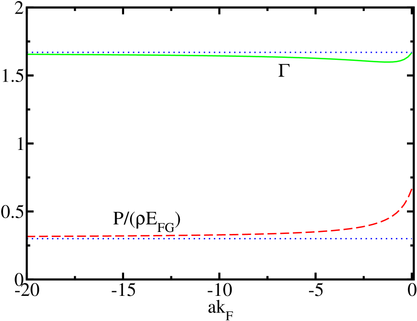
The pressure () and the adiabatic index () of the superfluid gas in the range are shown in Fig. 12. For noninteracting Fermi gas (), and we have and . In the limit we can use the low density expansion (Eq. 1) to obtain
| (35) |
In the limit, we have , therefore
| (36) |
where according to the present calculations.
The calculated value of is at and decreases monotonously to as . However, The adiabatic index , is for both and , and has a minimum value of at .
V CONCLUSIONS
The present work shows that accurate calculations of the pairing gaps and energies of superfluid Fermi gases are possible with the fixed node GFMC method. The unknown nodal surfaces can be determined variationally by minimizing the fixed node GFMC energy. This method gives the exact result in the (Fermi gas) and (BEC of molecules) limits for short range attractive interaction, and seems to overcome the fermion sign problem. An alternative method based on path integral Monte Carlo simulations is also being developed shumway et al. (2000).
Our results are in qualitative agreement with the known BCS-BEC crossover model (see Leggett Leggett (1980)) where gap and chemical potential() are calculated self consistently. The gap is determined as the minimum of the Bogoliubov quasiparticle energy , where is the single particle excitation energy and is the gap parameter. Two limiting cases were considered in this referenced article. For , , the minimum of occurs at and the minimum quasiparticle energy = . However, for , , the minimum of is at , and its value because . The BCS-BEC crossover takes place when and this corresponds to positive and of the order 1. The odd-even staggering given by Eq. 33 presumably equals the minimum quasiparticle energy in the limit .
According to Leggett’s description, in the weak BCS superfluids the ground state of systems with odd number of particles is expected to have momentum , while in the molecular liquid with BEC it is expected to have zero momentum. With this criteria the calculated values of (Table 2) suggest that the BCS to BEC transition occurs in the range . It appears to be a smooth transition or crossover.
A recent experiment by Bartenstein et al. also seems to corroborate some of our findings. In fact, in their paper Bartenstein et al. (2003) BCS-BEC crossover regime for 6Li is reported to be . In addition, in the unitary limit () they measured which includes within its range our result .
We can notice that in the BCS regime is much smaller than , while in the BEC regime . However, in the transition region is significantly larger than .
VI ACKNOWLEDGEMENTS
The work of J.C. is supported by the U. S. Department of energy under contract No. W-7405-ENG-36, while that of S.Y.C. and V.R.P is partly supported by U.S. National Science Foundation via Grant No. PHY-00-98353.


| -1 | 10 | 1.00 | 0.05 | 0 | 0 | 0 | NA |
|---|---|---|---|---|---|---|---|
| 14 | 1.00 | 1.00 | 0.010 | 0 | 0 | NA | |
| 20 | 1.00 | 1.00 | 0.104 | 0.024 | 0 | NA | |
| -3 | 10 | 0.40 | 0.165 | 0.019 | 0.009 | 0.002 | 1.13 |
| 14 | 0.28 | 0.280 | 0.020 | 0.006 | 0.003 | 1.05 | |
| -10 | 10 | 0.295 | 0.096 | 0 018 | 0.007 | 0.002 | 0.48 |
| 14 | 0.220 | 0.130 | 0.019 | 0.007 | 0.003 | 0.44 | |
| 10 | 0.315 | 0.103 | 0.020 | 0.010 | 0.003 | 0.50 | |
| 14 | 0.181 | 0.102 | 0.024 | 0.006 | 0.004 | 0.44 |
| N=11,13 | N=15,17,19 | |
| 0 | 1 | 2 |
| -1 | 1 | 2 |
| -3 | 1 | 2 |
| -10 | 1 | 1 |
| 1 | 1 | |
| 10 | 1 | 1 |
| 3 | 1 | 1 |
| 2 | 0 or 1 | 0 or 1 |
| 1 | 0 | 0 |
| 0.75 | 0 | 0 |
| 0.5 | 0 | 0 |
| 0 | 0.99(4) | 0.44(1) | 0 | ||
| 0.1 | 1.03(5) | 0.34(1) | -0.01(1) | 3.69 | 44.3 |
| 1.37(5) | 0.02(1) | -0.20(1) | 1.21 | 14.5 | |
| 0.5 | 1.80(5) | -0.33(1) | -0.49(1) | 0.74 | 8.9 |
| 1.0 | 3.2(1) | -2.23(1) | -2.31(1) | 0.38 | 4.6 |
| 5.7(3) | -4.58(2) | -4.63(1) | 0.28 | 3.4 | |
| 2.0 | 14.0(5) | -12.84(3) | -12.86(1) | 0.19 | 2.3 |
References
- cooper (1959) L. N. Cooper, R. L. Mills,and A. M. Sessler, Phys. Review 114, 1377 (1959).
- Pethick and Ravenhall (1995) C. J. Pethick and D. G. Ravenhall, Ann. Rev. Nuc. Part. Science 45, 429 (1995).
- Leggett (1980) A. J. Leggett, in Modern Trends in the Theory of Condensed Matter, edited by A. Pekalski and R. Przystawa (Springer-Verlag, Berlin, 1980).
- Randeria (1995) M. Randeria, in Bose-Einstein Condensation, edited by A. Griffin, D. Snoke, and S. Stringari (Cambridge, 1995).
- Gorkov and Melik-Barkhudarov (1961) L. P. Gorkov and T. K. Melik-Barkhudarov, Sov. Phys. JETP 13, 1018 (1961).
- De Marco et al. (1999) B. De Marco, and D. S. Jin, Science 285, 1703 (1999).
- O’Hara et al. (2002) K. M. O’Hara, S. L. Hemmer, M. E. Gehm, S. R. Granade, and J. E. Thomas, Science 298, 2179 (2002).
- Stenger et al. (1999) J. Stenger, S. Inouye, M. R. Andrews, H.-J. Miesner, D. M. Stamper-Kurn, and W. Ketterle, Phys. Rev. Lett. 82, 2422 (1999).
- Roberts et al. (2001) J. L. Roberts, N. R. Claussen, S. L. Cornish, E. A. Donley, E. A. Cornell, and C. E. Wieman, Phys. Rev. Lett. 86, 4211 (2001).
- Regal et al. (2003) C. A. Regal, C. Ticknor, J. L. Bohn, and D. S. Jin, Nature 424, 47 (2003).
- Regal et al. (2004) C. A. Regal, M. Greiner, and D. S. Jin, Phys. Rev. Lett. 92, 040403 (2004).
- Lenz (1929) W. Lenz, Z. Physik 56, 778 (1929).
- Huang (1957) K. Huang, and C. N. Yang, Phys. Rev. 105, 767 (1957).
- Baker (1999) G. A. Baker, Phys. Rev. C 60, 054311 (1999).
- Heiselberg (2001) H. Heiselberg, Phys. Rev. A 63, 043606 (2001).
- Carlson et al. (2003) J. Carlson, S.-Y. Chang, V. R. Pandharipande, and K. E. Schmidt, Phys. Rev. Lett. 91, 50401 (2003).
- Pandharipande et al. (1973) V. R. Pandharipande, and H. A. Bethe, Phys. Rev. C 7, 1312 (1973).
- Cowell et al. (2002) S. Cowell, H. Heiselberg, I. E. Mazets, J. Morales, V. R. Pandharipande, and C. J. Pethick, Phys. Rev. Lett. 88, 210403 (2002).
- Schmidt et al. (1977) V. R. Pandharipande, and K. E. Schmidt, Phys. Rev. A 15, 2486 (1977).
- Kalos (1974) M. H. Kalos, D. Levesque, and L. Verlet, Phys. Rev. A 9, 2178 (1974).
- Anderson (1975) J. B. Anderson, J. Chem. Phys. 63, 1499 (1975).
- Bouchaud et al. (1988) J. P. Bouchaud, A. Georges, and C. Lhuillier, J. Physique 49, 553 (1988).
- petrov et al. (2003) D. S. Petrov, C. Salomon, and G. V. Shlyapnikov, cond-mat/0309010 (2003).
- shumway et al. (2000) J. Shumway, and D. M. Ceperley, Journ. de Phys. IV 10 (P5), 3-16 (2000).
- Bartenstein et al. (2003) M. Bartenstein, A. Altmeyer, S. Riedl, S. Jochim, C. Chin, J. H. Denschlag, and R. Grimm, Phys. Rev. Lett. 92, 120401-1 (2004).