Playing Games with the Quantum Three-Body Problem

Abstract

Quantum mechanics courses focus mostly on its computational aspects. This alone does not provide the same depth of understanding as most physicists have of classical mechanics. The understanding of classical mechanics is significantly bolstered by the intuitive understanding that one acquires through the playing of games like baseball at an early age. It would be good to have similar games for quantum mechanics. However, real games that involve quantum phenomena directly are impossible. So, computer simulated games are good alternatives. Here a computer game involving three interacting quantum particles is discussed. It is hoped that such games played at an early age will provide the intuitive background for a better understanding of quantum mechanics at a later age.

1 Introduction

“…and then the wavefunction collapses.” What visual images are inspired by such a statement? We can visualize collapsing bridges, buildings and maybe even a soufflé. But collapsing wavefunctions are a visual mystery for both novices and experts in quantum mechanics. A few years of graduate school can teach a physics student the mathematical methods as well as the experimental tests of quantum mechanics. However, acquiring an intuitive understanding of the subject is more challenging. Classical mechanics is easier to understand due to the ready availability of visual images (collapsing bridges, soufflés, etc.). It is also significant that these images of classical mechanics are observed by everyone at an early age making them part of our intuition. Similar early introductions to quantum phenomena would be very useful for the learning experience of children. They would build a foundation for later, more rigorously mathematical, presentations of quantum mechnics. However, real visual images for quantum mechanics are difficult to find. So let us look for some computer simulated visual images through a computer game based on quantum mechanics.

Using computers for physics education has become quite mainstream through the last decade[1, 2, 3, 4]. However, using physics based computer games is not that common[5, 6]. Personally, I prefer the game approach for several reasons. It can provide an intuitive understanding at a very early age without the need for mathematics. It is non-threatening and develops physics intuition in a relaxed setting. It is like understanding projectile motion while playing baseball. In particular, for quantum mechanics, computer games are uniquely useful as real games like baseball shed very little light on the subject.

In the past, I have developed a game based on the quantum mechanical free particle (“Quantum Duck Hunt”)[7, 8]. Here, I present a significantly more complex system – an interacting three particle system. The game based on this system is called “Quantum Focus”[9]. It deals with various subtle aspects of quantum observation and wavefunction collapse[10].

This game is not meant to teach quantum mechanics to college students. It is meant to develop “quantum intuition” at a much earlier age (maybe elementary school). Children playing this kind of games are expected to develop “gut feelings” about quantum phenomena just as they usually do for classical phenomena by playing baseball or soccer. The approach here is not that of standard accepted padagogy. Something different is being tried to see if it works better. I have tried it on a few children (my own and their friends!). The results are very encouraging – now they want to learn quantum mechanics! If we wait until college to develop quantum intuition in youngsters, we might miss the formative years when most intuition is developed. However, college students may also benefit from this game by studying the computer code and trying to come up with their own variations.

2 The game

The game is started by choosing “Start” from the “Action” menu. Three boxes colored red, green and blue appear on a black background screen. With time, the color of each box begins to smear into neighboring boxes (see figure 1).

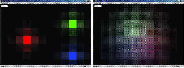
Figure 1: The game screen at starting time (left) and at a later time (right).

At the same time, the brightest spot in each color smear moves away from the other two. As the colors spread, they produce mixtures of the primary colors in various proportions in different boxes on the screen.

The object of the game is to make each color smear as small as possible and at the same time bring the three colors as close together as possible. The only tool available for achieving this is the click of the mouse at strategic points. Clicking the mouse will retract a color completely into a single box – the one that was clicked. But this retraction or “collapse” will occur only with a probability proportional to the preexisting intensity of that color in that box. So, if there is very little red in a certain box, it is unlikely that red can be collapsed into it by any amount of clicking. This is why, sometimes, a click of the mouse may produce no effect at all. An interesting sound effect will accompany the actual collapse of a color.

The quantum mechanically minded readers must already have noted that the three primary colors represent three particles. The intensity of a primary color is related to the probability of finding the corresponding particle at a given place. The mouse clicks simulate a particle detector’s attempts at detecting a particle. The retraction of a color into a single box simulates a wavefunction collapse. In the present model, the three particles are tied together by attractive forces. So, it is a bit tricky to see why quantum mechanics makes the three color smears move apart. This effect will be discussed later.

A score is computed in each time step. It depends on how small each color smear is and how close the three colors are. So, the goal is to produce a single white box and no other colored boxes. But this state of perfection can be seen to be impossible. The score displayed (at the top left corner) is the maximum score achieved during the course of a game.

It should be noted that, while the colors spread, nothing is lost. Colors that spread off-screen on one edge reappear on the opposite edge. This effect may be used for game strategies.

The game can be played at four levels of difficulty. The scoring formula respects the level of difficulty. The features of these levels will be discussed later.

3 The quantum three particle problem

This game is based on the quantum dynamics of three interacting distinguishable particles. Most quantum problems deal with the solution of the time-independent Schrödinger equation. But here we are concerned with the wavefunction collapse and subsequent change in the wavefunction. Hence, it is necessary to solve the time-dependent Schrödinger equation[10].

Let the positions of the three particles be ${\bf q}_{i}$, and their momenta be ${\bf p}_{i}$ ($i=1,2,3.$). Let the wavefunction of the system be $\psi(\{{\bf q}_{i}\},t)$ and its hamiltonian $H(\{{\bf q}_{i}\},\{{\bf p}_{i}\})$ where $t$ is time. Then the time-dependent Schrödinger equation to be solved is[12, 13]

$$i\hbar\frac{\partial\psi}{\partial t}=H\psi$$ (1)

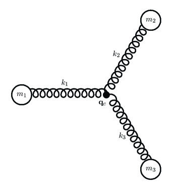
Figure 2: Three particles attached by “springs”

For simplicity I choose harmonic (“spring”) potentials to represent the interparticle forces (see figure 2). Also, The springs are assumed to have zero unextended length. The resulting hamiltonian is as follows.

$$H=\sum_{i=1}^{3}\frac{{\bf p}_{i}^{2}}{2m_{i}}+\sum_{i=1}^{3}\frac{k_{i}}{2}({\bf q}_{i}-{\bf q}_{c})^{2},$$ (2)

where $m_{i}$ is the mass and $k_{i}$ the spring constant for the $i^{\mbox{th}}$ particle. ${\bf q}_{c}$ is the position of the common center at which the three springs are tied.

It can be seen that, like most three particle problems, this cannot be separated in variables. The dependence on ${\bf q}_{c}$ complicates the hamiltonian significantly as it is not an independent coordinate. ${\bf q}_{c}$ depends on the particle coordinates due to the following zero net force condition.

$$\sum_{i=1}^{3}k_{i}({\bf q}_{i}-{\bf q}_{c})=0,$$ (3)

which gives

$${\bf q}_{c}=\frac{\sum_{j=1}^{3}k_{j}{\bf q}_{j}}{\sum_{j=1}^{3}k_{j}}.$$ (4)

Hence,

$$H=\sum_{i=1}^{3}\frac{{\bf p}_{i}^{2}}{2m_{i}}+\sum_{i=1}^{3}\frac{k_{i}}{2}\left({\bf q}_{i}-\frac{\sum_{j=1}^{3}k_{j}{\bf q}_{j}}{K}\right)^{2},$$ (5)

where $K=\sum_{j=1}^{3}k_{j}$.

Equation 1 can be solved numerically to obtain the time development of the wavefunction provided an intial value is specified. At any point in this time development, if a particle detector detects the first particle in a small region $R$, it will be with a probability

$$P_{1}=\int_{R}d^{3}{\bf q}_{1}\int_{-\infty}^{\infty}d^{3}{\bf q}_{2}\int_{-\infty}^{\infty}d^{3}{\bf q}_{3}\psi^{*}(\{{\bf q}_{i}\},t)\psi(\{{\bf q}_{i}\},t).$$ (6)

If the particle is actually detected, the wavefunction must collapse to

$$\psi_{c}(\{{\bf q}_{i}\},t)=A\Delta_{R}({\bf q}_{1}-{\bf q}_{0})\psi(\{{\bf q}_{i}\},t),$$ (7)

where $\Delta_{R}({\bf q}_{1}-{\bf q}_{0})$ is a sharply peaked function that is nonzero only in the region of detection $R$ centered about the position ${\bf q}_{0}$. The detailed form of this function depends on the detector sensitivity in the region $R$. In the limit $R\rightarrow 0$, it is the Dirac delta function:

$$\lim_{R\rightarrow 0}\Delta_{R}({\bf q}_{k}-{\bf q}_{0})=\delta^{3}({\bf q}_{k}-{\bf q}_{0}).$$ (8)

The constant $A$ is needed to renormalize $\psi$ after the collapse. The detection of the other two particles can be described similarly.

After the collapse, $\psi$ is replaced by $\psi_{c}$ and the time development continued as given by equation 1 until the next collapse.

4 The numerical technique

The computer screen being 2-dimensional, the above formulation will be reduced to its 2-dimensional equivalent for the purpose of the game. To use standard finite difference methods, the screen space is divided into a matrix of $m$ columns and $n$ rows to produce a total of $m\times n$ boxes. For the purpose of a game, we may sacrifice accuracy for speed as long as the qualitative aspects of the system are maintained. So, the maximum values of $m$ and $n$ are chosen to be 12 and 8.

To solve the Schrödinger equation, boundary conditions must be specified. There are several possible natural choices:

1. Perfectly reflecting boundary conditions.

2. Perfectly absorbing boundary conditions.

3. Periodic boundary conditions.

The perfectly reflecting boundary produces a discontinuity at the boundary that interferes with visualization. The perfectly absorbing boundary allows particles to go off screen, thus making them useless for visualization. The periodic condition seems to be the best for visualization. It identifies the left edge to the right and the bottom edge to the top (toroidal topology). Hence, particle current that disappears on one edge reappears on the opposite edge.

The discrete forms for the $x$ and $y$ components of each coordinate ${\bf q}_{i}$ may be written as

$$q_{ix}=a_{ix}\Delta x,\;\;\;\;q_{iy}=a_{iy}\Delta y,$$ (9)

where $i=1,2,3$, $a_{ix}=0,1,2,\ldots,m-1$, and $a_{iy}=0,1,2,\ldots,n-1$. $\Delta x$ is the mesh width in the $x$ direction and $\Delta y$ is the mesh width in the $y$ direction. If the mesh width in time is $\Delta t$, then equation 1 produces the following recursive formula for the computation of $\psi$.

$$\psi(\{{\bf q}_{i}\},t)=(1-iH\Delta t/\hbar)\psi(\{{\bf q}_{i}\},t-\Delta t).$$ (10)

In general, the above numerical algorithm for the solution of the Schrödinger equation is known to be unstable[11]. However, we can use it in the present case because wavefunction collapses are expected to preempt any instability. Besides, as noted before we are not looking for high accuracy.

The wavefunction $\psi$, at one instant of time, is a function of all coordinates ${\bf q}_{i}$. So, its discretized form must depend on all $a_{ix}$ and $a_{iy}$. Thus, for numerical computation, $\psi$ is represented by an array of 6 dimensions (one for each $a_{ix}$ and $a_{iy}$). In the notation of the C language it would be: $\psi[a_{1x}][a_{1y}][a_{2x}][a_{2y}][a_{3x}][a_{3y}]$. For compactness of notation I can write this as: $\psi[a][b][c][d][e][f]$ or $\psi_{a,b,c,d,e,f}$. Then the finite difference form of the operation by the hamiltonian $H$ is found from equation 5 using equation 9 and the following finite difference forms of the ${\bf p}_{i}^{2}$ operators.

$${\bf p}_{1}^{2}\psi_{a,b,c,d,e,f} = -\hbar^{2}\left(\frac{\psi_{a+1,b,c,d,e,f}-2\psi_{a,b,c,d,e,f}+\psi_{a-1,b,c,d,e,f}}{(\Delta x)^{2}}+\right.$$

$$\left.+\frac{\psi_{a,b+1,c,d,e,f}-2\psi_{a,b,c,d,e,f}+\psi_{a,b-1,c,d,e,f}}{(\Delta y)^{2}}\right),$$

$${\bf p}_{2}^{2}\psi_{a,b,c,d,e,f} = -\hbar^{2}\left(\frac{\psi_{a,b,c+1,d,e,f}-2\psi_{a,b,c,d,e,f}+\psi_{a,b,c-1,d,e,f}}{(\Delta x)^{2}}+\right.$$

$$\left.+\frac{\psi_{a,b,c,d+1,e,f}-2\psi_{a,b,c,d,e,f}+\psi_{a,b,c,d-1,e,f}}{(\Delta y)^{2}}\right),$$

$${\bf p}_{3}^{2}\psi_{a,b,c,d,e,f} = -\hbar^{2}\left(\frac{\psi_{a,b,c,d,e+1,f}-2\psi_{a,b,c,d,e,f}+\psi_{a,b,c,d,e-1,f}}{(\Delta x)^{2}}+\right.$$ (11)

$$\left.+\frac{\psi_{a,b,c,d,e,f+1}-2\psi_{a,b,c,d,e,f}+\psi_{a,b,c,d,e,f-1}}{(\Delta y)^{2}}\right).$$

Here the most common finite difference form for second derivatives is used. Using equations 5, 9, and 11 in equation 10, the wavefunction for successive time steps can be computed. The numerical method chosen here does not maintain normalization of $\psi$. Hence, after each time step computation, $\psi$ must be normalized[11].

Also after each time step computation, the screen image must be updated to provide an animated visual effect. The RGB coloring scheme on the computer screen provides a natural way of representing the three particle probabilities. The red, green and blue color intensities in a box are made proportional to the probabilities of finding each of the three particles in that box. The discretized version of equation 6 provides the probabilities to be used. They are as follows.

$$P_{1} = \sum_{c,d,e,f}\psi^{*}_{a,b,c,d,e,f}\psi_{a,b,c,d,e,f},$$

$$P_{2} = \sum_{a,b,e,f}\psi^{*}_{a,b,c,d,e,f}\psi_{a,b,c,d,e,f},$$

$$P_{3} = \sum_{a,b,c,d}\psi^{*}_{a,b,c,d,e,f}\psi_{a,b,c,d,e,f}.$$ (12)

So, the C++ code used to find the amount of red color (particle 1) in a box is as follows.

int CQFocusDoc::Red(int a, int b)
{
      int c, d, e, f;
      float red = 0;

      for(c=0;c<xpts;c++)
            for(d=0;d<ypts;d++)
                  for(e=0;e<xpts;e++)
                        for(f=0;f<ypts;f++)
                              red += norm(Psi[a][b][c][d][e][f]);

      return(255*sqrt(sqrt(red))); //Square root used to enhance
                                   //color for better visibility.
}

The amounts of the other two colors are computed similarly.

When the mouse button is clicked in a box, one of the three particles is picked randomly for collapse and then the decision to actually collapse it is made based on the probability given by equation 12. The following C++ code fragment makes these probabilistic decisions.

partnum = MyRandom(3); //Generates an integer random number between 0 and 2.
intensity = MyRandom(256);
intensity = (intensity*intensity*intensity)/(256*256);
// The above redifinition improves game by requiring less mouse clicking.

i = point.x/bwidth; // x pixel position divided by box width.
j = point.y/bheight; // y pixel position divided by box height.

switch(partnum)
{
case 0:
  if(intensity < pDoc->Red(i,j)) // Function Red(i,j) defined above.
    { pDoc->Collapse(partnum, CPoint(i,j)); setcollapse = true;}
  break;
case 1:
  if(intensity < pDoc->Green(i,j))
    { pDoc->Collapse(partnum, CPoint(i,j)); setcollapse = true;}
  break;
case 2:
  if(intensity < pDoc->Blue(i,j))
    { pDoc->Collapse(partnum, CPoint(i,j)); setcollapse = true;}
  break;
}

The wavefunction after the collapse is given by equation 7. The function $\Delta_{R}({\bf q}_{k}-{\bf q}_{0})$ in its discrete form is chosen as the discrete form of the Dirac delta function:

$$\Delta_{R}({\bf q}_{k}-{\bf q}_{0})=\left\{\begin{array}[]{ll}1,&\mbox{if $a_{kx}=a_{0x}$ and $a_{ky}=a_{0y}$}\\ 0,&\mbox{otherwise},\end{array}\right.$$ (13)

where the integer values $a_{kx}$, $a_{0x}$, $a_{ky}$ and $a_{0y}$ are defined as in equation 9. So, the C++ code for wavefunction collapse is as follows.

void CQFocusDoc::Collapse(int partnum, CPoint point)
{
  int a, b, c, d, e, f;
  switch(partnum)
  {
  case 0:
    for(a=0;a<xpts; a++)
      for(b=0;b<ypts;b++)
        for(c=0;c<xpts;c++)
          for(d=0;d<ypts;d++)
            for(e=0;e<xpts;e++)
              for(f=0;f<ypts;f++)
              {
                if(a!=point.x || b!=point.y)
                  Psi[a][b][c][d][e][f] = 0;
              }
    break;
  case 1:
    for(a=0;a<xpts; a++)
      for(b=0;b<ypts;b++)
        for(c=0;c<xpts;c++)
          for(d=0;d<ypts;d++)
            for(e=0;e<xpts;e++)
              for(f=0;f<ypts;f++)
              {
                if(c!=point.x || d!=point.y)
                  Psi[a][b][c][d][e][f] = 0;
              }
    break;
  case 2:
    for(a=0;a<xpts; a++)
      for(b=0;b<ypts;b++)
        for(c=0;c<xpts;c++)
          for(d=0;d<ypts;d++)
            for(e=0;e<xpts;e++)
              for(f=0;f<ypts;f++)
              {
                if(e!=point.x || f!=point.y)
                  Psi[a][b][c][d][e][f] = 0;
              }
    break;
  }
  Normalize();
}

Here partnum gives the randomly picked particle number and point identifies the box clicked.

5 The levels of difficulty

The game can be played at four different levels of difficulty. The difficulty level is increased by increasing the values of the spring constants $k_{i}$. This increases the rate at which the positions of maximum probability move apart. The reason will be seen in the next section.

The difficulty level is increased also by reducing the total number of boxes. This increases the speed of computation and hence increases the rate of spreading of the wavefunction.

The score allows for higher difficulty levels.

6 Some results

The primary purpose of this game is to provide repeated and consistent visual effects that mimic quantum wavefunction dynamics. As expected, the wavefunction collapse leaves the undetected particles unaffected. Also as expected, the probability profile of each particle spreads with time. The resulting mix of the primary colors produces some rather unusual color effects that may interest the artists amongst us. What is not-so-obvious is as follows. If we start with one particle in a collapsed state (with no velocity), with time its probability peak moves away from those of the other particles! As the potential function used here is attractive, this is somewhat surprising. However, closer scrutiny can explain this phenomenon.

Consider the standard one-particle harmonic oscillator. Higher energy eigenstates have probability peaks farther away from the origin. This means that particles that start off with higher momenta are likely to have their probability peaks farther away. For the present case, a particle collapsed to its position eigenstate has high probabilities for large momenta and hence, large energy. This makes its probability peak move away from the other particles.

References

- [1] D. M. Cook, Comput. Phys. 11, 240-245; 331-335 (1997).
- [2] R. Ehrlich, M. Dworzecka, and W. M. MacDonald, Comput. Phys. 6, 90-96 (1992).
-
[3]
W. Christian, See Physlets at
http://webphysics.davidson.edu/Applets/Applets.html. -
[4]
See Visual Quantum Mechanics by KSU Physics Education Group at
http://web.phys.ksu.edu/vqm/software/.(Not all software at this site work correctly). - [5] T. Biswas, Comput. Phys. 8, 446-450 (1994).
- [6] T. Biswas, Comput. Phys. 12, 488-492 (1998).
- [7] T. Biswas, Computing in Science and Engineering, 3, 84-88, (2001).
-
[8]
The game “Quantum Duck
Hunt” (Microsoft Windows software) can be found at the URL:
www.engr.newpaltz.edu/~biswast. -
[9]
The game “Quantum Focus” (Microsoft Windows software)
can be found at the URL:
www.engr.newpaltz.edu/~biswast. - [10] T. Biswas, eprint arXiv:quant-ph/0311079 (2003).
- [11] W. H. Press, S. A. Teukolsky, W. T. Vetterling, B. P. Flannery, Numerical Recipes in C (second edition, Cambridge University Press, 1992) pp. 851-853.
- [12] R. Shankar, Principles of Quantum Mechanics (Plenum Press).
-
[13]
T. Biswas, Quantum Mechanics – Concepts and
Applications, (available at the URL:
www.engr.newpaltz.edu/~biswast).