Benchmarking Iterative Projection Algorithms for Phase Retrieval

Abstract

Iterative projection algorithms for phase retrieval are tested on two simple ‘toy’ models. The result provides useful insights in the behavior of these algorithms.

Iterative transform methods pioneered by Gerchberg and Saxton Gerchberg:1972 , are well established techniques for iteratively recovering the phase from the knowledge of the diffraction amplitude. The development of iterative algorithms with feedback in the early nineteen-eighties by Fienup produced a remarkably successful optimization method capable of extracting phase information from adequately sampled intensity data fienup:1978 ; fienup:1982 ; cederquist:1988 . Finally, the important theoretical insight that these iterations may be viewed as projections in Hilbert space stark:1984 ; stark:1987 has allowed theoreticians to analyze and improve on the basic Fienup algorithm elser:2003 ; luke:1 ; luke:2 ; luke:3 .

These algorithms try to find the intersection between two sets, typically the set of all the possible objects with a given diffraction pattern (modulus), and the set of all the objects that are constrained within a given area called support (or solvent in crystallography). The search for the intersection is based on the information obtained by ‘projecting’ the current estimate on the two sets. An error metric exists to characterize the distance between the current estimate and a given feasibility set. The error metric and its gradient are used in conjugate gradient (CG) based methods such as SPEDEN speden . A projector $\bm{P}$ is an operator that takes to the closest point of a set from the current point $\rho$. A repetition of the same projection is equal to one projection alone ($\bm{P^{2}}=\bm{P}$). Another operator used here is the reflector $\bm{R}=2\bm{P}-\bm{I}$. We consider two sets, $S$ (support) and $M$ (modulus). The support constraint is convex, while the modulus constraint is non-convex. Problems arise for non-convex sets, where projections become multivalued luke:siam .

The support projector $\bm{P}_{s}$ acts on the object density $\rho$ by setting to 0 the density of the object outside a given region. The modulus projector $\bm{P}_{m}$ acts on the density $\rho$ in the Fourier domain $\tilde{\rho}$ by forcing the modulus $|\tilde{\rho}|$ to be equal to the known one $m$, but keeping the phase of the current object in the Fourier domain $\tilde{\rho}$. This operator is demonstrated to be a projector on the non-covex set of the magnitude constraint luke:siam . The same paper discusses the problems of multi-valued projections for non-convex sets, which do not statisfy the requirements for gradient-based minimization algorithms, and the related nonsmoothness of the squared set distance metric, which may lead to numerical instabilities. See also luke:siam1 for a follow-up discussion on the non-smooth analysis.

Several algorithms based on these concepts have now been proposed and a visual representation of their behaviour is usefull to characterize the algorithm in various situations, in order to help chose the most appropriate one for a particular problem.

The following algorithms require a starting point $\rho^{0}$, which is generated by assigning a random phase to the measured object amplitude in the Fourier domain $|\tilde{\rho}|$. The first algorithm called Error Reduction (ER) (Gerchberg and Saxton Gerchberg:1972 ) (see also Alternating Projections Onto Convex Sets bregman:1965 or Alternating Projections Onto Nononvex Sets stark:1984 ) is simply:

$$\rho^{(n+1)}=\bm{P_{s}P_{m}}\rho^{(n)\,,}$$ (1)

by projecting back and forth between two sets, it converges to the local minimum (gradient type). The eigenvalues of the support projectors are 0 and 1, with corrisponding eigenvectors the pixels outside and inside the support. Replacing the support projector $\bm{P}_{s}$ with its reflector $\bm{R}_{s}=2\bm{P}_{s}-\bm{I}$, the corrisponding eigenvalues become -1 and 1, i.e. the charge density $\rho$ outside the support is multiplied by -1. This algorithm is called solvent flipping in crystallography abrahams:1996 :

$$\rho^{(n+1)}=\bm{R_{s}P_{m}}\rho^{(n)}\,.$$ (2)

The Hybrid Input Output (HIO) fienup:1978 ; fienup:1982 is

$$\rho^{(n+1)}(x)=\begin{cases}\bm{P_{m}}\rho^{(n)}(x)&\text{if $x\in S$}\\ (\bm{I}-\beta\bm{P_{m}})\rho^{(n)}(x)&\text{otherwise}\end{cases}$$ (3)

It is often used in conjunction of the ER algorithm, alternating several HIO iterations and one ER iteration (HIO(20)+ER(1) in our case). Difference Map with $\gamma_{1}=-\beta^{-1}$, $\gamma_{2}=\beta^{-1}$ elser:2003 , which requires 4 projections (two time-consuming modulus constraint projections):

$$\rho^{(n+1)}=\{ \bm{I} +\bm{P_{S}}\left[\left(\beta+1\right)\bm{P_{m}}-\bm{I}\right]$$ (4)

$$- \bm{P_{m}}\left[\left(\beta-1\right)\bm{P_{s}}+\bm{I}\right]\}\rho^{(n)}$$

The Averaged Successive Reflections (ASR) luke:1 is:

$$\rho^{(n+1)}=\tfrac{1}{2}[\bm{R_{s}R_{m}}+\bm{I}]\rho^{(n)}$$ (5)

The Hybrid Projection Reflection (HPR) luke:2 is derived from a relaxation of ASR:

$$\rho^{(n+1)} = [\bm{R_{s}}\left(\bm{R_{m}}+(\beta-1)\bm{P_{m}}\right)$$ (6)

$$+ \bm{I}+(1-\beta)\bm{P_{m}}]\rho^{(n)}$$

It is equivalent to HIO if positivity is not enforced but it is written in a recursive form, instead of a case by case form such as Eq. 3. Finally Relaxed Averaged Alternating Reflectors RAAR (previously named RARS) luke:3

$$\rho^{(n+1)}=\left[\tfrac{1}{2}\beta\left(\bm{R_{s}R_{m}}+\bm{I}\right)+(1-\beta)\bm{P_{m}}\right]\rho^{(n)}$$ (7)

For $\beta=1$, HIO, HPR, ASR and RAAS coincide.

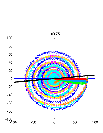
Figure 1: The basic features of the iterative projection algorithms can understood by this simple model of two lines intersecting (1). The aim is to find the intersection. The ER algorithm and the Solvent flipping algorithms converge in some gradient type fashion (the distance to the two sets never increases), with the solvent flip method being slightly faster when the angle between the two lines is small. HIO and variants move slightly in the direction where the gap between the two projections decreases, but at the same time in the direction of the gap, following a spiral path. When the two lines do not intersect (1, HIO and variants keep moving in the direction of the gap. ER, Solvent Flipping and RAAR converge at (or close to) the local minimum.

The first test is performed on the simplest possible case: find the intersection between two lines. Fig. 1 shows the behavior of the various algorithms, The two sets are represented by a horizontal blue line (support) and a tilted black line (modulus). ER simply projects back and forth between these two lines, and moves along the support line in the direction of the intersection. Solvent Flip projects onto the modulus, ‘reflects’ on the support, and moves along the reflection of the modulus constraint onto the support. The solvent flipping algorithm is slightly faster than ER due to the increase in the angle of the projections and reflections. HIO and variants (ASR, Difference Map, HPR and RAAS) move in a spiral around the intersection eventually reaching the intersection. For similar $\beta$ RAAS behaves somewhere in between ER and HIO with a sharper spiral, reaching the solution much earlier. Alternating 20 iteration of HIO and 1 of ER (HIO(20)+ER(1)) considerably speeds up convergence.

When a gap is introduced between the two lines (Fig. 1) so that the two lines do not intersect, HIO and variants move away from this local minimum in search for another ‘attractor’ or local minimum. This shows how these algorithms escape from local minima and explore the Hilbert space for other minima. ER, Solvent Flip, RAAS converges to or near the local minimum. By varying $\beta$ RAAS becomes a local minimizer for small $\beta$, and becomes like HIO for $\beta\simeq 1$. ER, solvent flip HIO+ER converge to the local minimum. The properties of SPEDEN cannot be fully apreciated in these examples since the support constraint is represented by a one dimensional set, and this conjugate gradient method is designed for multidimensional minimization. However it is important to remark that such algorithm converges quadratically to the local minimum, reaching the intersection in a single step when it exists, and the local minimum when a gap is introduced between the two sets in fewer steps than any of the other algorithm described here.

A more realistic example is shown in Fig. 2. Here the circumference of two circles represent the modulus constraint, while the support constraint is represented by a line. The two circles are used to represent a non-convex set with a local minimum. It is difficult to represent a true modulus constraint in real space. For a representation of the modulus constraint in reciprocal space see luke:siam . The advantage of this example is the simplicity in the ‘modulus’ projector operator (it projects onto the closest circle). Although a real modulus constraint projector is not as simple as the one used in this example, there are similarities: each Fourier space point provides an n-dimensional ellipsoid type equation.

We start from a position near the local minimum. ER, solvent flip and HIO+ER all fall into this trap (Fig. 2), although increasing the interval between ER iterations in the HIO+ER algorithm would allow it to escape this local minimum. HIO and variants move away from the local minimum, ‘find’ the other circle, but converge to the center of the circle, with all but Diff. Map. not reaching a solution. In the center of the circle the projection on the modulus constraint becomes ‘multivalued’, and its distance metric is ‘nonsmooth’. The introduction of a small a random number added to the resulting solution at every step allows all the HIO-type codes to escape stagnation and find the solution (Fig. 2). The random number can be as low as the numerical precision of the computer. For $\beta$ reduced to $.9$, RAAS would not reach the solution, but converge close to the local minimum. As a latest test in this series Fig. 2, shows the behaviour of the algorithms when the support is tangent to the circle, the two solutions coincide, and the the two constraints are parallel. The only algorithm to reach the solution is RAAS, but HIO+ER would also reach the solution if the interval between ER steps was sufficiently large.

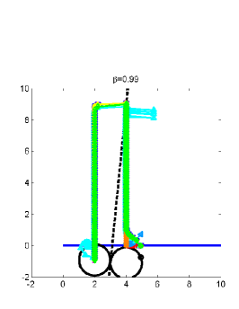
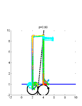
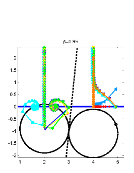
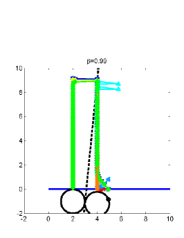
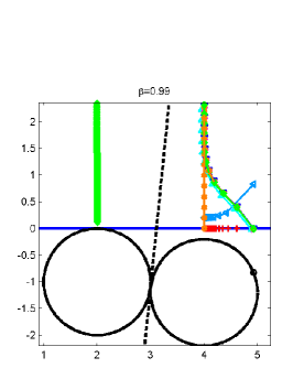
Figure 2: The horizontal line represents a support constraint, while the two circles represent a non convex constraint, i.e. the modulus constraint. The dashed line divides the region closer to one circle from the other. The starting point is on the circle to the right, possessing a local minimum distance to the line. (a) The gradient-type (ER and Solvent Flip) algorithms converge to the local minimum, while HIO and variants move away from the local minimum in the direction of the gap (vertical) untill they reach the region where the second circle is closer (delimited by the dashed line). From here they try to move in the same spiral-like path of the two lines (Fig. 1) untill they reach the point where the projecton on the circle and the line are parallel, and start moving toward the the center of the circle which has the correct solution. They stagnate in the center of the circle where the projection is multivalued. Only the Diff. Map reaches one of the two solutions. The addition of a small value of the order of the numerical precision after each iteration solves this stagnation (b). When one of the circles just touches the other constraint most algorithms either get stuck near the local minimum or stagnate. RAAS is the only one that reaches the vicinity of the solution (c).

I Positivity

The situation changes slightly when we consider the positivity constraint. The previous definitions of the algorithms still apply just replacing $\bm{P}_{S}$ with $\bm{P}_{S+}$:

$$\bm{P}_{S+}=\begin{cases}\rho(x)\ &\text{if $x\in S$ and $\rho(x)\geq 0$}\\ 0&\text{otherwise.}\end{cases}$$ (8)

The only difference is HIO which becomes:

$$\rho^{(n+1)}=\begin{cases}\bm{P_{m}}\rho^{(n)}(x)&\text{if $x\in S$ and $\bm{P_{m}}\rho^{(n)}(x)\geq 0$}\\ (1-\beta\bm{P_{m}})\rho^{(n)}&\text{otherwise.}\end{cases}$$ (9)

Fig. 3 shows that HIO bouches at the $x=0$ axis. As the positivity constraint gets closer to the solution, none of the algorithms converges to the solution (Fig. 3), with the HIO-type algorithms bouncing between the regions closer to the two circles. Only Difference Map for $\beta>1$ converges (Fig. 3). Also HIO+ER would reach the solution for larger intervals between ER iterations.

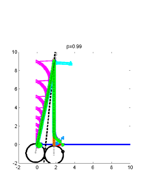
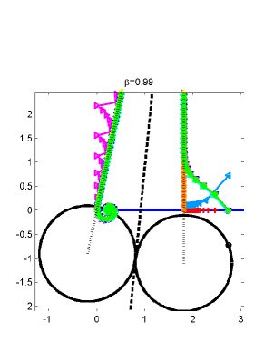
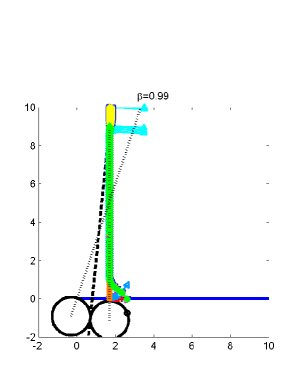
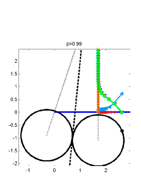
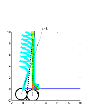
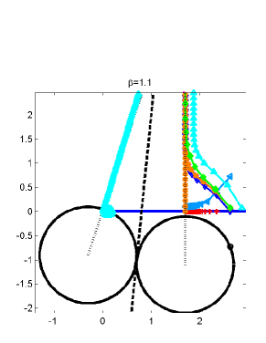
Figure 3: (a) The starting point is again on the circle to the right, close to a local minimum. HIO and variant move away from the local minimum in the direction of the gap untill they reach the region where the circle to the left is closer. Instead of moving in a spiral like fashon, the iterations move close to the dotted line joining the center of the left circle to the origin, except for HIO that bounches on the x=0 axis. (b) The solution is very close to 0, and the dotted line originating from the circle to the left and passing by the origin becomes more tilted. The various algorithms after moving in the vertical direction away from the local minimum, reach the dashed line and start moving toward the tilted dotted line, falling back in the region closer to the first minimum. Tthese algorithms bounce between the regions closer to each circle without reaching the solution. With $\beta>1$, i.e. inverting the order of the operators, Diff. Map converges, and RAAS diverges, while HIO HPR and ASR stagnate.

II Conclusions

ER is a simple but powerfull local minimizer, HIO and variants are very powerfull in escaping local minima, but in several situations fail to converge. When positivity is introduced, the recursive version of HIO (HPR) converges more ‘smoothly’ to the solution without bounching on the $x=0$ axis. Alternating between HIO and ER with the correct intervals would have worked in all the examples shown above. RAAS is a good (single parameter) way to change from ‘global’ to local minimizer, although it seems better to start from a high value of $\beta$ and decrease it afterwards. Difference Map is succesfull in a few more of the examples shown above for the proper choiche of $\beta$, however it involves 2 time consuming modulus constraint operations. To find when stagnation occours one can monitor the distances (using the proper error metrics) of the current solution before and after aplying various projectors, or monitor the autocorrelation between two succesive reconstructions. SPEDEN, a conjugate gradient based method, reaches a local minimum with quadradic convergence, and provides such kind of information.

The Solvent flipping algorithm does not show much success in the examples shown above. Despite this it was used to improve images abrahams:1996 , and in a modified form to solve 3D structures ab-initio chargeflip . Perhaps the reason for the latter success has more to do with the threshold constraint used. A threshold projector multiplies by 0 everything that is below a given threshold, while a threshold reflector multiplies it by -1. The application of this constraint has been proven succesfull in obtaining ab-initio solution in many circumstances applied in a variety of ways. Apart from Charge Flipping, which uses a threshold reflector chargeflip , in electron density modification procedure with SIR giacovazzo:preprint , in atomicity constraint Elser:acta , a modified histogram constraint using the Difference Map (H. He, private comm.), and for complex valued objects, in the shrink-wrap algorithm using an updated support constraint by thresholding the current object reconstruction at low resolution marchesini:prbr .

By compressing the image in small spots and by increasing the flat region, these algorithms based on the threshold constraint resemble the maximum entropy method maxent , which tries to reduce the amout of information in an image and maximize the number of pixels of equal value (solvent).

What distinguishes shrink-wrap and SIR algorithms is that they somehow solve the low resolution first, and gradually introduce high resolution information while slowly updating the low resolution information. Fienup has also shown that starting from a low resolution image, slowly increasing resolution improves the algorithm fienup:1990 . Also SPEDEN starting from a low resolution target has been shown to slowly extend the correct phase information to higher resolution. One possible explanation could be that the set based on low resolution is ‘more smooth’. Perhaps also slowly increasing the gray levels in an image, or the number of possible phases of its Fourier transform could improve convergence by gradually introducing more degrees of freedom in the resulting image, although a set defined by ‘quantized’ levels is also non-convex rendering it counterproductive.

- (1) R. Gerchberg and W. Saxton, Optik 35, 237 (1972).
- (2) J. R. Fienup, Opt. Lett. 3, 27-29 (1978).
- (3) J. R. Fienup, Appl. Opt. 21, 2758 (1982).
- (4) J. N. Cederquist, J. R. Fienup, J. C. Marron, R. G. Paxman, Opt. Lett. 13, 619. (1988).
- (5) A. Levi and H. Stark, J. Opt. Soc. Am. A1, 932-943 (1984).
- (6) H. Stark, Image Recovery: Theory and applications. (Academic Press, New York, 1987).
- (7) V. Elser, J. Opt. Soc. Am. A20, 40 (2003).
- (8) H. H. Bauschke, P. L. Combettes, and D. R. Luke. J. Opt. Soc. Am. A19, 1334-1345 (2002).
- (9) H. H. Bauschke, P. L. Combettes, and D. R. Luke, J. Opt. Soc. Am. A20, 1025-1034 (2003).
- (10) D. R. Luke, (2003) [PIMS-03-13].
- (11) S. P. Hau-Riege, H. Szöke, H. N. Chapman et al. (2004) [arXiv:physics.optics/0403091]
- (12) D. R. Luke, J. V. Burke, R. G. Lyon, SIAM Review 44 169-224 (2002).
- (13) D. R. Luke, J. V. Burke, R. G. Lyon, SIAM J. Contr. Opt. 42, 576-595 (2003).
- (14) L. M. Brègman, Sov. Math. Dokl. 6, 688-692 (1965).
- (15) J. P. Abrahams, A. W. G. Leslie, Acta Cryst. D52, 30-42 (1996)
- (16) V. Elser, Acta Cryst. A59, 201-209 (2003), [arXiv:cond-mat/0209690].
- (17) G. Oszlányi and A. Sütő, Acta Cryst. A60, 134-141 (2004) [arXiv:cond-mat/0308129]
- (18) B. Carrozzini, G. L. Cascarano, L.De Caro, et al. [arXiv:physics.optics/0404073]
- (19) S. Marchesini et al. Phys. Rev. B68, 140101(R) (2003) [arXiv:physics.optics/0306174]
- (20) G. Bricogne, Acta Cryst. A44, 517-545 (1988).
- (21) J. R. Fienup, A. M. Kowalczyk J. Opt. Soc. Am. A 7, 450 (1990).