Stochastic analysis of different rough surfaces

Abstract

This paper shows in detail the application of a new stochastic approach for the characterization of surface height profiles, which is based on the theory of Markov processes. With this analysis we achieve a characterization of the scale dependent complexity of surface roughness by means of a Fokker-Planck or Langevin equation, providing the complete stochastic information of multiscale joint probabilities. The method is applied to several surfaces with different properties, for the purpose of showing the utility of this method in more detail. In particular we show evidence of the Markov properties, and we estimate the parameters of the Fokker-Planck equation by pure, parameter-free data analysis. The resulting Fokker-Planck equations are verified by numerical reconstruction of the conditional probability density functions. The results are compared with those from the analysis of multi-affine and extended multi-affine scaling properties which is often used for surface topographies. The different surface structures analysed here show in detail the advantages and disadvantages of these methods.

1 Introduction

Among the great variety of complex and disordered systems the complexity of surface roughness is attracting a great deal of scientific interest Sayles1978 ; Vicsek1992-e ; Barabasi1995 ; Davies1999 ; Wendt2002a . The physical and chemical properties of surfaces and interfaces are to a significant degree determined by their topographic structure. Thus a comprehensive characterization of their topography is of vital interest from a scientific point of view as well as for many applications Dharmadhikari1999 ; Saitou2001 ; Sydow2003 .

Most popular methods used today for the characterization of surface roughness are based on the concepts of self-affinity and multi-affinity, where the multifractal $f(\alpha)$ spectrum has been regarded as the most complete characterization of a surface Feder1988 ; Family1991 ; Vicsek1992-e ; Barabasi1995 . One example of a measure of roughness which is commonly used in this context is the rms surface width $w_{r}(x)=\langle(h(\tilde{x})-\bar{h})^{2}\rangle^{1/2}_{r}$, where $h(\tilde{x})$ is the measured height at point $\tilde{x}$, $\langle\,\cdot\,\rangle_{r}$ denotes the average over an interval of length $r$ around the selected point $x$, and $\bar{h}$ the mean value of $h(\tilde{x})$ in that interval. Thus the roughness is measured at a specific location $x$ and over a specific scale $r$. Then a scaling regime of the ensemble average $\langle w_{r}\rangle$ in $r$, if it exists, is analyzed according to $\langle w_{r}^{\alpha}\rangle\sim r^{\xi_{\alpha}}$, usually $\alpha\in\mathds{Q}$. Here, $\langle\,\cdot\,\rangle$ denotes the mean over the available range in $x$. For a more thorough introduction into scaling concepts we refer the reader to the literature, e.g. Feder1988 ; Family1991 ; Vicsek1992-e ; Barabasi1995 . Terms concerning scaling concepts which are used in this paper are rapidly introduced in section 4. Here, we have to note the following points which concern stochastic aspects of roughness analysis: First, the ensemble average $\langle w_{r}\rangle$ must obey a scaling law as mentioned above, and second, the statistics of $w_{r}(x)$ are investigated over distinct length scales $r$, thus possible correlations between $w_{r}(x)$ and $w_{r^{\prime}}(x)$ on different scales $r,r^{\prime}$ are not examined.

In this paper we want to give a deeper introduction into a new approach to surface roughness analysis which has recently been introduced by us Friedrich1998a ; Waechter2003_plus_preprint and by Jafari2003 . This method is based on stochastic processes which should grasp the scale dependency of surface roughness in a most general way. No scaling feature is explicitly required, and especially the correlations between different scales $r$ and $r^{\prime}$ are investigated. To this end we present a systematic procedure as to how the explicit form of a stochastic process for the $r$-evolution of a roughness measure similar to $w_{r}(x)$ can be extracted directly from the measured surface topography. This stochastic approach turns out to be a promising tool also for other systems with scale dependent complexity such as turbulence Friedrich1998a ; Renner2001 ; Lueck1999 , financial data Friedrich2000a ; Ausloos2003 , and cosmic background radiation Ghasemi2003 . Also this stochastic approach has recently enabled the numerical reconstruction of surface topographies Jafari2003 .

Here we demonstrate our ansatz by analysing a number of data sets from different surfaces. The purpose is to show extensively the utility of this method for a wide class of rough surfaces. The examples show different kinds of scaling properties which are, in addition, briefly analysed. Among these examples is a collection of road surfaces measured with a specially designed profile scanner. Preliminary results of the analysis of one of these surfaces have already been presented Waechter2003_plus_preprint . AFM measurement data from an evaporated gold film have already been analysed in an earlier stage of the method Friedrich1998a . Since then, the method has been significantly refined and extended. Measurements of a steel crack surface were taken by confocal laser scanning microscopy (CLSM) Wendt2002a .

As a measure of surface roughness we use the height increment CenteredInc

$$h_{r}(x):=h(x+r/2)-h(x-r/2)$$ (1)

depending on the length scale $r$. For other scale dependent roughness measures, see Family1991 ; Barabasi1995 . The height increment $h_{r}$ is used because its moments, which are well-known as structure functions (see section 4), are closely connected with spatial correlation functions. Nevertheless, it should be pointed out that our method presented in the following could be easily generalized to any scale dependent measure, e.g. the above-mentioned $w_{r}(x)$ or wavelet functions Haase2003 . As a new ansatz, $h_{r}$ is regarded as a stochastic variable in $r$. Without loss of generality we consider the process as being directed from larger to smaller scales. The focus of our method is the investigation of how the surface roughness is linked between different length scales.

In the remainder of this paper we will first summarize in section 2 some central aspects of the theory of Markov processes which form the basis of our analysis procedure. Details concerning the measurement data are presented in section 3, their scaling properties are analyzed in section 4. The Markov properties of our examples are investigated in section 5. In section 6 we estimate for each data set the parameters of a Fokker-Planck equation. The ability of this equation to describe the statistics of $h_{r}$ in the scale variable $r$ is then examined in section 7, followed by concluding remarks in section 8.

2 Surface roughness as a Markov process

Complete information about the stochastic process would be available from the knowledge of all possible $n$-point, or more precisely $n$-scale, joint probability density functions (pdf) $p(h_{1},r_{1};h_{2},r_{2};\ldots;h_{n},r_{n})$ describing the probability of finding simultaneously the increments $h_{1}$ on the scale $r_{1}$, $h_{2}$ on the scale $r_{2}$, and so forth up to $h_{n}$ on the scale $r_{n}$. Here we use the notation $h_{i}(x)=h_{r_{i}}(x)$, see eq. (1). Without loss of generality we take $r_{1}<r_{2}<\ldots<r_{n}$. As a first question one has to ask for a suitable simplification. In any case the $n$-scale joint pdf can be expressed by multiconditional pdf

$$p(h_{1},r_{1};\ldots;h_{n},r_{n})=$$ (2)

$$p(h_{1},r_{1}|h_{2},r_{2};\ldots;h_{n},r_{n})\cdot p(h_{2},r_{2}|h_{3},r_{3};\ldots;h_{n},r_{n})$$

$${}\cdot\ldots\cdot p(h_{n-1},r_{n-1}|h_{n},r_{n})\cdot p(h_{n},r_{n})\,.$$

Here, $p(h_{i},r_{i}|h_{j},r_{j})$ denotes a conditional probability of finding the increment $h_{i}$ on the scale $r_{i}$ under the condition that simultaneously, i.e. at the same location $x$, on a larger scale $r_{j}$ the value $h_{j}$ was found. It is defined with the help of the joint probability $p(h_{i},r_{i};h_{j},r_{j})$ by

$$p(h_{i},r_{i}|h_{j},r_{j})=\frac{p(h_{i},r_{i};h_{j},r_{j})}{p(h_{j},r_{j})}\;.$$ (3)

An important simplification arises if

$$p(h_{i},r_{i}|h_{i+1},r_{i+1};\ldots;h_{n},r_{n})=p(h_{i},r_{i}|h_{i+1},r_{i+1})\;.$$ (4)

This property is the defining feature of a Markov process evolving from $r_{i+1}$ to $r_{i}$. Thus for a Markov process the $n$-scale joint pdf factorize into $n$ conditional pdf

$$p(h_{1},r_{1};\ldots;h_{n},r_{n})=p(h_{1},r_{1}\,|h_{2},r_{2})$$ (5)

$${}\cdot\ldots\cdot p(h_{n-1},r_{n-1}\,|h_{n},r_{n})\cdot p(h_{n},r_{n})\;.$$

The Markov property implies that the $r$-dependence of $h_{r}$ can be regarded as a stochastic process evolving in $r$, driven by deterministic and random forces. Here it should be noted that if condition (4) holds this is true for a process evolving in $r$ from large down to small scales as well as the reverse from small to large scales Renner2001Diss . Equation (5) also emphasizes the fundamental meaning of conditional probabilities for Markov processes since they determine any $n$-scale joint pdf and thus the complete statistics of the process.

For any Markov process a Kramers-Moyal expansion of the governing master equation exists Risken1984 . For our height profiles it takes the form

$$-r\,\frac{\partial}{\partial r}\;p(h_{r},r|h_{0},r_{0})\,=$$ (6)

$$\sum_{k=1}^{\infty}\left(-\frac{\partial}{\partial h_{r}}\right)^{k}D^{(k)}(h_{r},r)\,p(h_{r},r|h_{0},r_{0})\,.$$

The minus sign on the left side of eq. (6) expresses the direction of the process from larger to smaller scales, furthermore the factor $r$ corresponds to a logarithmic variable $\rho=\ln r$ which leads to simpler results in the case of the scaling behaviour FPE . To derive the Kramers-Moyal coefficients $D^{(k)}(h_{r},r)$, the limit $\Delta r\rightarrow 0$ of the conditional moments has to be performed:

$$D^{(k)}(h_{r},r)=\lim_{\Delta r\rightarrow 0}M^{(k)}(h_{r},r,\Delta r)\,,\qquad\mbox{where}$$ (7)

$$M^{(k)}(h_{r},r,\Delta r)=$$ (8)

$$\frac{r}{k!\Delta r}\int_{\scriptscriptstyle-\infty}^{\scriptscriptstyle+\infty}(\tilde{h}-h_{r})^{k}\,p(\tilde{h},r-\Delta r|h_{r},r)\,d\tilde{h}\,.$$

The moments $M^{(k)}(h_{r},r,\Delta r)$ characterize the alteration of the conditional probability $p(h_{r},r|h_{0},r_{0})$ over a finite step size $\Delta r=r_{0}-r$ and are thus also called “transitional moments”.

A second major simplification is valid if the noise included in the process is Gaussian distributed. In this case the coefficient $D^{(4)}$ vanishes (from eqs. (7) and (8) it can be seen that $D^{(4)}$ is a measure of non-gaussianity of the included noise). According to Pawula’s theorem, together with $D^{(4)}$ all the $D^{(k)}$ with $k\geq 3$ disappear and the Kramers-Moyal expansion (6) collapses to a Fokker-Planck equation Risken1984 , also known as Kolmogorov equation Kolmogorov1931 :

$$-r\,\frac{\partial}{\partial r}\;p(h_{r},r|h_{0},r_{0})\,=$$

$$\left\{-\frac{\partial}{\partial h_{r}}D^{(1)}(h_{r},r)+\frac{\partial^{2}}{\partial h_{r}^{2}}D^{(2)}(h_{r},r)\right\}p(h_{r},r|h_{0},r_{0})$$

The Fokker-Planck equation then describes the evolution of the conditional probability density function from larger to smaller length scales and thus also the complete $n$-scale statistics. The term $D^{(1)}(h_{r},r)$ is commonly denoted as the drift term, describing the deterministic part of the process, while $D^{(2)}(h_{r},r)$ is designated as the diffusion term, determined by the variance of a Gaussian, $\delta$-correlated noise (compare also eqs. (7) and (8)).

By integrating over $h_{0}$ it can be seen that the Fokker-Planck equation (2) is also valid for the unconditional probabilities $p(h_{r},r)$ (see also section 7). Thus it covers also the behaviour of the moments $\langle h_{r}^{n}\rangle$ (also called structure functions) including any possible scaling behaviour. An equation for the moments can be obtained by additionally multiplying with $h_{r}^{n}$ and integrating over $h_{r}$

$$-r\frac{\partial}{\partial r}\langle h_{r}^{n}\rangle=$$

$$n\langle D^{(1)}(h_{r},r)h_{r}^{n-1}\rangle+n(n-1)\langle D^{(2)}(h_{r},r)h_{r}^{n-2}\rangle\;.$$

For $D^{(1)}$ being purely linear in $h_{r}$ ($D^{(1)}=\alpha h_{r}$) and $D^{(2)}$ purely quadratic ($D^{(2)}=\beta h_{r}^{2}$), the multifractal scaling $\langle h_{r}^{n}\rangle\sim r^{\xi_{n}}$ with $\xi_{n}=n\alpha+n(n-1)\beta$ is obtained from (2). If in contrast $D^{(2)}$ is constant in $h_{r}$, a monofractal scaling where $\xi_{n}$ are linear in $n$ may occur, see Friedrich1998a .

Lastly, we want to point out that the Fokker-Planck equation (2) corresponds to the following Langevin equation (we use Itô’s definition) Risken1984

$$-\frac{\partial h_{r}}{\partial r}=D^{(1)}(h_{r},r)/r+\sqrt{D^{(2)}(h_{r},r)/r}\,\Gamma(r)\;,$$ (11)

where $\Gamma(r)$ is a Gaussian distributed, $\delta$-correlated noise. The use of this Langevin model in the scale variable opens the possibility to directly simulate surface profiles with given stochastic properties, similar to Jafari2003 .

With this brief summary of the features of stochastic processes we have fixed the scheme from which we will present our analysis of diverse rough surfaces. There are three steps: First, the verification of the Markov property. Second, the estimation of the drift and diffusion coefficients $D^{(1)}$ and $D^{(2)}$. Third, the verification of the estimated coefficients by a numerical solution of the corresponding Fokker-Planck equation, thus reconstructing the pdf which are compared to the empirical ones.

3 Measurement data

With the method outlined in section 2 we analysed a collection of road surfaces measured with a specially designed profile scanner as well as two microscopic surfaces, namely an evaporated gold film and a crack surface of a low-alloyed steel sample, as already mentioned in section 1.

The road surfaces have been measured with a specially designed surface profile scanner. The Longitudinal resolution was 1.04$\,\mathrm{mm}$, the profile length being typically 20$\,\mathrm{m}$ or 19000 samples, respectively. Between ten and twenty parallel profiles with a lateral distance of 10$\,\mathrm{mm}$ were taken for each surface, see fig. 1. The vertical error was always smaller than 0.5$\,\mathrm{mm}$ but in most cases approximately 0.1$\,\mathrm{mm}$. Details can be found in Waechter2002a .

For the Au film data, the surface of four optical glass plates had been coated with an Au layer of 60$\,\mathrm{nm}$ thickness by thermal evaporation Friedrich1998a . The topography of these films was measured by atomic force microscopy at different resolutions, resulting in a set of images of $256\times 256$ pixels each, where every pixel specifies the surface height relative to a reference plane, see fig. 5. Out of these images 99 could be used for the analysis presented here, resulting in about $6.5\cdot 10^{6}$ data points. Sidelengths vary between 36$\,\mathrm{nm}$ and 2.8$\,\mathrm{\mu m}$.

The sample of the crack measurements was a fracture surface of a low-alloyed steel (german brand 10MnMoNi5-5). A detailed description of the measurements can be found in Wendt2002a . Three CLSM (Confocal Laser Scanning Microscopy) images of size 512x512 pixels in different spatial resolutions were available, see fig. 9. Pixel sizes are 0.49, 0.98, and 1.95$\,\mathrm{\mu m}$, resulting in image widths of 251, 502, and 998$\,\mathrm{\mu m}$, repectively. Unavoidable artefacts of the CLSM method were removed by simply omitting for each image those data with the smallest and largest height value, similar to Wendt2002a . Nevertheless this cannot guarantee the detection of all the artefacts. The possible consequences are discussed together with the results.

For the analysis in the framework of the theory of Markov processes, we will normalize the measurement data by the quantity $\sigma_{\infty}$ defined by

$$\sigma_{\infty}^{2}=\lim_{r\rightarrow\infty}\langle h_{r}^{2}\rangle\,.$$ (12)

Thus it is possible to obtain dimensionless data with a normalization independent of the scale $r$, in contrast to e.g. $\sigma_{r}^{2}=\langle h_{r}^{2}\rangle$. As a consequence the results, especially $M^{(k)}(h_{r},r,\Delta r)$ and $D^{(k)}(h_{r},r)$ (cf. section 2), will also be dimensionless. From the definition it is easy to see that $\sigma_{\infty}$ can be derived via $\sigma_{\infty}^{2}=2\sigma_{x}^{2}=2\langle(h(x)-\bar{h})^{2}\rangle$ if $h(x)$ becomes uncorrelated for large distances $r$.

4 Scaling analysis

In this paper a number of examples was selected from all data sets under investigation. Because most popular methods of surface analysis are based on scaling features of some topographical measure, the examples were chosen with respect to their different scaling properties as well as their results from our analysis based on the theory of Markov processes.

In the analysis presented here we use the well-known height increment $h_{r}(x)$, which has been defined in eq. 1, as a scale-dependent measure of the complexity of rough surfaces CenteredInc . Scaling properties are reflected by the $r$-dependence of the so-called structure functions

$$S^{n}(r)=\langle|h_{r}^{n}|\rangle\,.$$ (13)

If one then finds

$$S^{n}(r)\sim r^{\xi_{n}}$$ (14)

for a range of $r$, this regime is called the scaling range. In that range the investigated profiles have self-affine properties, i.e., they are statistically invariant under an anisotropic scale transformation. If furthermore the dependence of the exponents $\xi_{n}$ on the order $n$ is nonlinear, one speaks of multi-affine scaling. Those properties are no longer identified by a single scaling exponent, but an infinite set of exponents. A detailed explanation of self- and multi-affine concepts is beyond the scope of this article. Instead, we would like to refer the reader to the literature Feder1988 ; Family1991 ; Vicsek1992-e ; Barabasi1995 . The power spectrum, which often is used to determine scaling properties, can easily be derived from the second order structure function. It is defined as the Fourier transform of the autocorrelation function $R(r)$, which itself is closely related to $S^{2}(r)$ by $R(r)=\langle h(x)^{2}\rangle-S^{2}(r)/2$, by comparing eqs. (1) and (13).

In addition to the $r$-dependence of the structure functions, a generalized form of scaling behaviour can be determined analogously to the Extended Self Similarity (ESS) method which is popular in turbulence research Benzi1993 . When the $S^{n}(r)$ are plotted against a structure function of specific order, say $S^{3}(r)$, in many cases an extended scaling regime is found according to

$$S^{n}(r)\sim\left(S^{3}(r)\right)^{\zeta_{n}}\,.$$ (15)

Clearly, meaningful results are restricted to the regime where $S^{3}$ is monotonous. It is easy to see that now the $\xi_{n}$ can be obtained by

$$\xi_{n}=\zeta_{n}\cdot\xi_{3}\,,$$ (16)

cf. Benzi1993 . While for turbulence it is widely accepted that by this means experimental defiencies can be compensated to some degree, for surface roughness the meaning of ESS lies merely in a generalized form of scaling properties.

It should be noted that the results of any scaling analysis may be influenced by the method of measurement, by the definition of the roughness measure, here $h_{r}(x)$ (or $w_{r}(x)$ as mentioned in section 1), as well as by the algorithms used for the analysis Wendt2002a ; Alber1998a . Nevertheless, this problem is not addressed here as the main focus of our investigations is the application of the theory of Markov processes to experimental data.

4.1 Surfaces with scaling properties

In fig. 1 we present road surface data with different kinds of scaling properties. For each data set a short profile section is shown. Structure functions of order one to six on double logarithmic scale are presented in fig. 2. Following the arguments in Renner2001 , higher order structure functions cannot be evaluated with sufficient precision from the given amount of data points. The worn asphalt pavement (Road 1) is an example of a comparably large scaling regime over more than one order of magnitude in $r$. A surface with similar features, namely a cobblestone road, has already been presented in Waechter2003_plus_preprint . Two separate scaling regions are found for a Y-shaped concrete stone pavement (Road 2). Additionally a sharp notch can be seen in the structure functions at $r=0.2\,\mathrm{m}$, indicating a strong periodicity of the pavement caused by the length of the individual stones. The third example, a “pebbled concrete” pavement (Road 3), consists of concrete stones with a top layer of washed pebbles. This material is also known as “exposed aggregate concrete”. Here, the scaling region of the structure functions is only small. For the basalt stone pavement (Road 4), being the fourth example, scaling properties are poor. We have nevertheless marked a possible scaling range and derived the respective scaling exponents for comparison with the other examples. Similar to the Y-shaped concrete stones, a periodicity can be found at about 0.1$\,\mathrm{m}$ length scale.

Figure 1: Measurement data from selected road surfaces with different kinds of scaling properties. Pavements are worn asphalt (Road 1), Y-shaped concrete stones (Road 2), pebbled concrete stones (Road 3), and basalt stones (Road 4), from top to bottom. For each surface a short section of the respective height profile is shown.

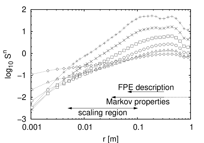
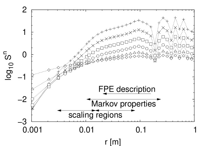
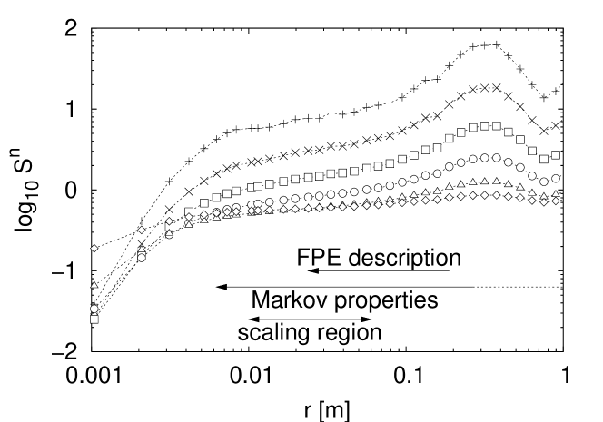
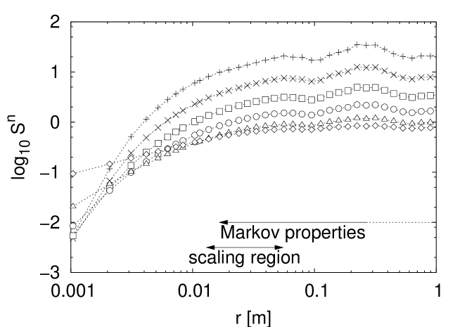
Figure 2: Structure functions $S^{n}(r)$ of selected road surfaces (see fig. 1) with different kinds of scaling properties on a log-log scale (see text). Symbols correspond to orders $n$; diamonds ($n=1$), triangles ($n=2$), circles ($n=3$), squares ($n=4$), x signs ($n=5$), and plus signs ($n=6$).

The results for the generalized scaling behaviour according to eq. (15) are shown in fig. 3. It can be seen that indeed for three of the surfaces in fig. 1 an improved scaling behaviour is found by this method. Only for Road 4 do the generalized scaling properties remain weak. In fig. 4 the scaling exponents $\xi_{n}$ of the structure functions within the marked scaling regimes in fig. 2 were determined and plotted against the order $n$ as open symbols. Additionally, values of $\xi_{n}$ were derived according to eqs. (15) and (16) and added as crosses. For Road 2 two sets of exponents correspond to the two distinct scaling regimes in fig. 2. Even though there is only one set of $\zeta_{n}$ found in fig. 3, two sets of $\xi_{n}$ are obtained due to the two different $\xi_{3}$, see eqs. (14) and (16).

All surfaces from fig. 1 show a more or less nonlinear dependence of the $\xi_{n}$ on $n$, indicating multi-affine scaling properties. The scaling exponents obtained via the generalized scaling according to eq. (15) are in good correspondence with the $\xi_{n}$ achieved by the application of eq. (14). Deviations are seen for Road 2 and at higher orders for Road 3, possibly caused by inaccuracies in the fitting procedure. For Road 4 no generalized scaling is observed (compare fig. 3) and thus values of $\xi_{n}$ cannot be derived from $\zeta_{n}$. From this we conclude that scaling properties for some cases are questionable as a comprehensive tool to characterize the complexity of a rough surface.

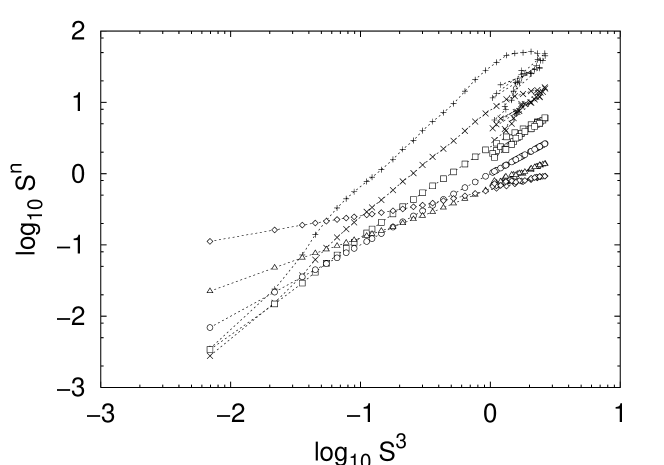
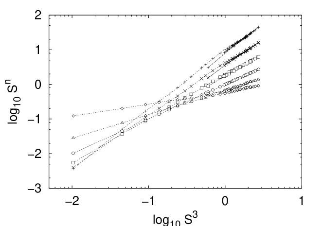
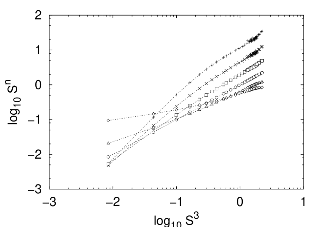
Figure 3: Generalized scaling analysis of the surfaces shown in fig. 1. Structure functions $S^{n}$ are displayed versus $S^{3}$ on a log-log scale. Symbols correspond to orders $n$ as in fig. 2.

Figure 4: Scaling exponents $\xi_{n}$ of the surfaces shown in fig. 1 achieved via eq. (14) (open symbols) and those obtained via $\zeta_{n}$ from eq. (16) (crosses). For Road 2 two sets of exponents were obtained from the two scaling regimes found for $S^{n}(r)$ in fig. 2.

An example for good scaling properties is the gold film surface (Au). To increase statistical accuracy, increments are evaluated here in the direction of the rows of the images as well as the columns. In fig. 5 two of the 99 images under investigation are shown. Figure 6 presents the structure functions $S^{n}(r)$, derived from all images. The surface is randomly covered with granules which show no typical diameter. A scaling regime of more than one order of magnitude in $r$ is found for the structure functions $S^{n}(r)$ in fig. 6. Generalized scaling behaviour is clearly present as shown in fig. 7(a). The scaling exponents $\xi_{n}$ presented in part (b) of the same figure are nearly linear in $n$, thus this surface can not be regarded as multi-affine, but appears to be self-affine. Here, the $\xi_{n}$ achieved via eq. (16) match perfectly those obtained from eq. (15).

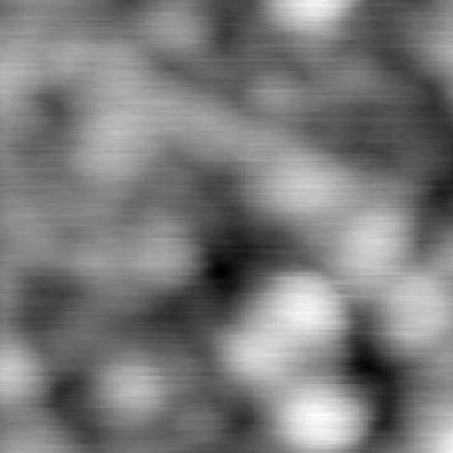
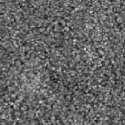
Figure 5: AFM images of the Au film surface. Sidelengths are 110$\,\mathrm{nm}$ and 1.1$\,\mathrm{\mu m}$. The relative surface height is represented as gray level. Maximum heights are 7.2$\,\mathrm{nm}$ and 13.3$\,\mathrm{nm}$, respectively.

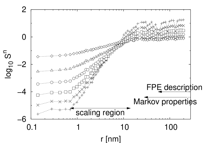
Figure 6: Structure functions $S^{n}(r)$ of the Au film surface on a log-log scale. Symbols correspond to orders $n$ as in fig. 2.

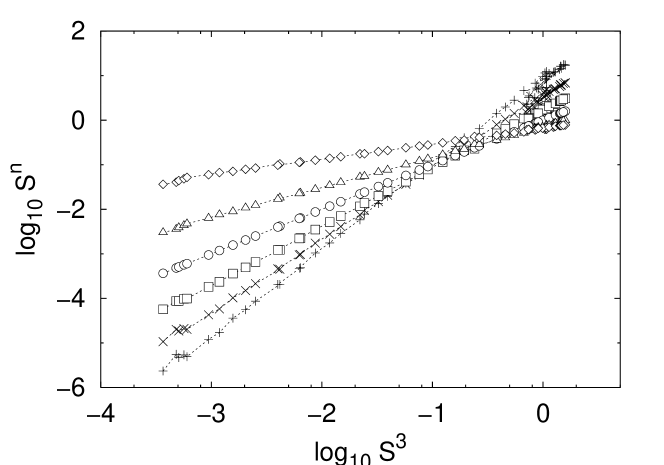
Figure 7: Generalized scaling properties (a) and scaling exponents (b) of the Au film surface shown in fig. 5. Scaling exponents $\xi_{n}$ achieved via eq. (15) are marked by open symbols, those obtained via $\zeta_{n}$ from eq. (16) by crosses. Compare also with fig. 3.

4.2 Surfaces without scaling properties

To complete the set of examples, we present two surfaces without scaling properties. The first one is a smooth asphalt road (Road 5), shown in fig. 8. No power law can be detected for the $S^{n}(r)$ but a generalized scaling is observed in fig. 11(a). The range of values of $S^{3}$, however, is relatively small.

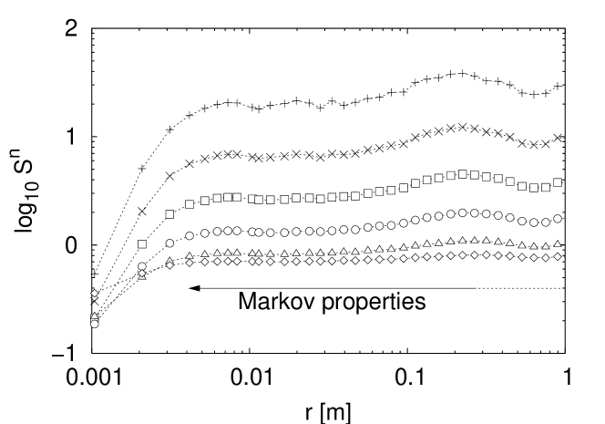
Figure 8: Measurement data (a) and structure functions (b) from a road surface without scaling properties (Road 5). The pavement is smooth asphalt. See also figs. 1 and 2.

The second example lacking a scaling regime is the steel fracture surface (Crack). One of the three CLSM images under investigation is shown in fig. 9(a). Figure 9(b) presents an additional REM image at a higher resolution, which gives an impression of the surface morphology. For the structure functions in fig. 10 no scaling properties are found, and the dependences of $S^{n}(r)$ on $S^{3}(r)$ in fig. 11(b) also deviate from proper power laws. It should be noted that in general scaling properties not only depend on the respective data set but also on the analysis procedure. Using other measures than $h_{r}(x)$, in Wendt2002a scaling regimes of those measures have been found, and scaling exponents could be obtained.

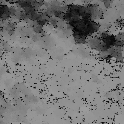
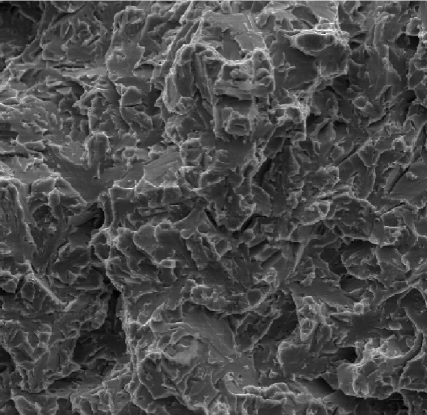
Figure 9: Measurement data from a steel crack surface (Crack). (a) CLSM image, side length 502$\,\mathrm{\mu m}$, (b) REM image, side length 140$\,\mathrm{\mu m}$.

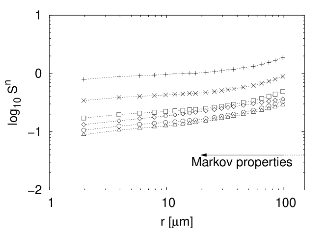
Figure 10: Structure functions $S^{n}(r)$ of the CLSM images from a steel crack surface (Crack) on a log-log scale. The symbols correspond to orders $n$ as in fig. 2.

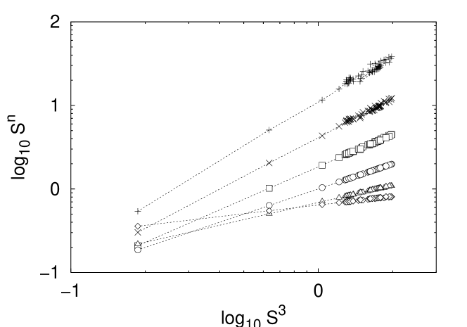
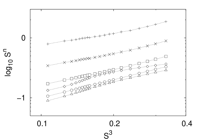
Figure 11: Generalized scaling properties of the surfaces shown in figs. 8 (Road 5 (a)) and 9 (Crack (b)). Compare also with figs. 3 and 7.

4.3 Conclusions on scaling analysis

To conclude the scaling analysis of our examples, we have chosen surfaces with a range of different scaling properties from good scaling over comparably wide ranges, such as for Road 1 and Au, to the absence of scaling, such as for Road 5 and Crack. The generalized scaling analysis, analogous to ESS Benzi1993 , leads to the same scaling exponents as the dependence of the structure functions $S^{n}(r)$ on the scale $r$, with some minor deviations.

5 Markov properties

As outlined in sections 1 and 2, we want to describe the evolution of the height increments $h_{r}(x)$ in the scale variable $r$ as realizations of a Markov process with the help of a Fokker-Planck equation. Consequently, the first step in the analysis procedure has to be the verification of the Markov properties of $h_{r}(x)$ as a stochastic variable in $r$.

For a Markov process the defining feature is that the $n$-scale conditional probability distributions are equal to the single conditional probabilities, according to eq. (4). With the given amount of data points the verification of this condition is only possible for three different scales. Additionally the scales $r$ are limited by the available profile length. For the sake of simplicity we will always take $r_{3}-r_{2}=r_{2}-r_{1}=\Delta r$. Thus we can test the validity of eq. (4) in the form

$$p(h_{1},r_{1}|\,h_{2},r_{1}\!+\!\Delta r)=p(h_{1},r_{1}|\,h_{2},r_{1}\!+\!\Delta r;h_{3}=0,r_{1}\!+\!2\Delta r)\,.$$ (17)

Note that in eq. (17) we take $h_{3}=0$ to restrict the number of free parameters in the pdf with double conditions.

Three procedures were applied to find out if Markov properties exist for our data. From the results of all three tests we will find a minimal length scale $l_{M}$ for which this is the case. The meaning of this so-called Markov length will be discussed below. In the following we will demonstrate the methods using the example of the Au surface.

5.1 Testing procedures

The most straightforward way to verify eq. (17) is the visual comparison of both sides, i.e., the pdf with single and double conditions. This is illustrated in fig. 12 for two different scale separations $\Delta r=17\,\mathrm{nm}$ and 35$\,\mathrm{nm}$. In each case a contour plot of single and double conditional probabilities $p(h_{1},r_{1}|h_{2},r_{2})$ and $p(h_{1},r_{1}|h_{2},r_{2};h_{3}\!\!=\!\!0,r_{3})$ is presented in the top panel of (a) and (b), respectively. Below two one-dimensional cuts at fixed values of $h_{2}\approx\pm\sigma_{\infty}$ are shown, representing directly $p(h_{1},r_{1}|h_{2}\!\!=\!\!\pm\sigma_{\infty},r_{2};h_{3}\!\!=\!\!0,r_{3})$. It can be seen that in panel (a), for the smaller value of $\Delta r$, the single and double conditional probability are different. This becomes clear from the crossing solid and broken contour lines of the contour plot as well as from the differing lines and symbols of the one-dimensional plots below. Panel (b), for $\Delta r=35$$\,\mathrm{nm}$, shows good correspondence of both conditional pdf. We take this finding as a strong hint that for this scale separation $\Delta r$ eq. (4) is valid and Markov properties exist. Following this procedure for all accessible values of $\Delta r$, the presence of Markov properties was examined. For this surface Markov properties were found for scale distances from $(25\pm 5)\,\mathrm{nm}$ upwards.

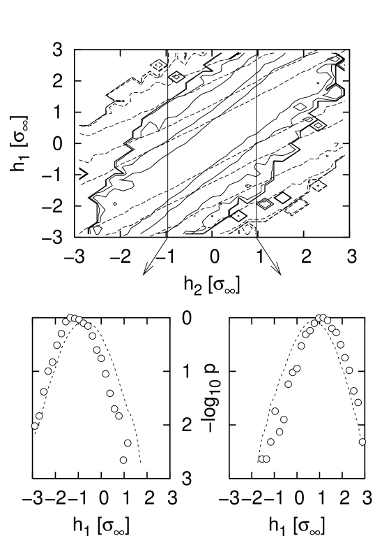
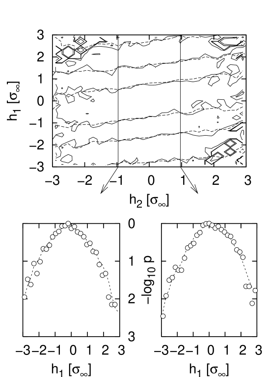
Figure 12: Test for Markov properties of Au film data for two different scale separations $\Delta r=14$$\,\mathrm{nm}$ (a) and $35$$\,\mathrm{nm}$ (b), where $\Delta r=r_{3}-r_{2}=r_{2}-r_{1}$ (see text). In both cases $r_{2}=169\,\mathrm{nm}$. In each case a contour plot of conditional probabilities $p(h_{1},r_{1}|h_{2},r_{2})$ (dashed lines) and $p(h_{1},r_{1}|h_{2},r_{2};h_{3}\!\!=\!\!0,r_{3})$ (solid lines) is shown in the top panel. Contour levels differ by a factor of 10, with an additional level at $p=0.3$. Below the top panels in each case, two one-dimensional cuts at $h_{2}\approx\pm\sigma_{\infty}$ are shown with $p(h_{1},r_{1}|h_{2},r_{2})$ as dashed lines and $p(h_{1},r_{1}|h_{2},r_{2};h_{3}\!\!=\!\!0,r_{3})$ as circles.

The validity of eq. (17) can also be be quantified mathematically using statistical tests. An approach via the well-known $\chi^{2}$ measure has been presented in Friedrich1998b , whereas in Renner2001 the Wilcoxon test has been used. Next, we give a brief introduction to this procedure, which will be used here, too. More detailed discussions of this test can be found in Bronstein1991 ; Renner2001 ; Renner2001Diss . For this procedure, we introduce the notation of two stochastic variables $x_{i},i=1,\ldots,n$ and $y_{j},j=1,\ldots,m$ which represent the two samples from which both conditional pdf of eq. (4) are estimated, i.e.

$$x(h_{r_{2}},r_{1},r_{2}) = h_{r_{1}}|_{h_{r_{2}}}$$

$$y(h_{r_{2}},h_{r_{3}},r_{1},r_{2},r_{3}) = h_{r_{1}}|_{h_{r_{2}};h_{r_{3}}}\;.$$ (18)

Here $\cdot|_{h_{x}}$ denotes the conditioning. All events of both samples are sorted together in ascending order into one sequence, according to their value. Now the total number of so called inversions is counted, where the number of inversions for a single event $y_{j}$ is just the number of events of the other sample which have a smaller value $x_{i}<y_{j}$. If eq. (17) holds and $n,m\geq 25$, the total number of inversions $Q$ is Gaussian distributed with

$$\langle Q\rangle = nm/2\quad\mathrm{and}$$

$$\sigma_{Q} = \sqrt{nm(n+m+1)/12}\;.$$ (19)

We normalize $Q$ with respect to its standard deviation and consider the absolute value

$$t=|Q-\langle Q\rangle|/\sigma_{Q}\;.$$ (20)

For its expectation value it is easy to show that $\langle t\rangle=\sqrt{2/\pi}$ (still provided that (17) is valid), where here the average $\langle\cdot\rangle$ is performed over $h_{2}$. If a larger value of $\langle t\rangle$ is measured for a specific combination of $r$ and $\Delta r$, we conclude that eq. (17) is not fulfilled and thus Markov properties do not exist. A practical problem with the Wilcoxon test is that all events $x_{i},y_{j}$ have to be statistically independent. This means that the intervals of subsequent height increments $h_{r}$ have to be separated by the largest scale involved. Thus the number of available data is dramatically reduced.

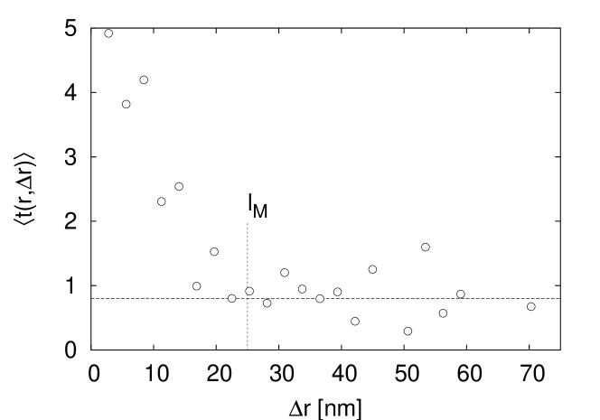
Figure 13: Wilcoxon test for the Au surface. The scale $r$ is 28$\,\mathrm{nm}$. The theroretically expected value $\langle t\rangle=\sqrt{2/\pi}$ is marked with a horizontal line, the Markov length $l_{M}=(25\pm 5)\,\mathrm{nm}$ with a vertical line.

In fig. 13 we present for the Au surface measured values of $\langle t(r,\Delta r)\rangle$ at a scale $r=28\,\mathrm{nm}$. The Markov length $l_{M}$ is marked where $\langle t(r,\Delta r)\rangle$ has approached its theroretical value $\sqrt{2/\pi}$.

Another method to show the validity of condition (17) is the investigation of the well-known necessary condition for a Markovian process, the validity of the Chapman-Kolmogorov equation Risken1984

$$p(h_{1},r_{1}|h_{3},r_{3})=\int_{-\infty}^{+\infty}p(h_{1},r_{1}|h_{2},r_{2})p(h_{2},r_{2}|h_{3},r_{3})\mbox{d}h_{2}\;.$$ (21)

We use this equation as a method to investigate the Markov properties of our data. This procedure was used for example in Friedrich1997a ; Friedrich1997b ; Ragwitz2001 ; Jafari2003 for the verification of Markov properties. It also served to show for the first time the existence of a Markov length in Friedrich1998b . The conditional probabilities in eq. (21) are directly estimated from the measured profiles. In fig. 14 both sides of the Chapman-Kolmogorov equation are compared for two different values of $\Delta r$. In an analogous way to fig. 12, for each $\Delta r$ the two conditional probabilities are presented together in a contour plot as well as in two cuts at fixed values of $h_{2}$. While for the smaller value $\Delta r=14$$\,\mathrm{nm}$ both the contour lines and the cuts at fixed $h_{2}$ clearly differ, we find a good correspondence for the larger value $\Delta r=35$$\,\mathrm{nm}$.

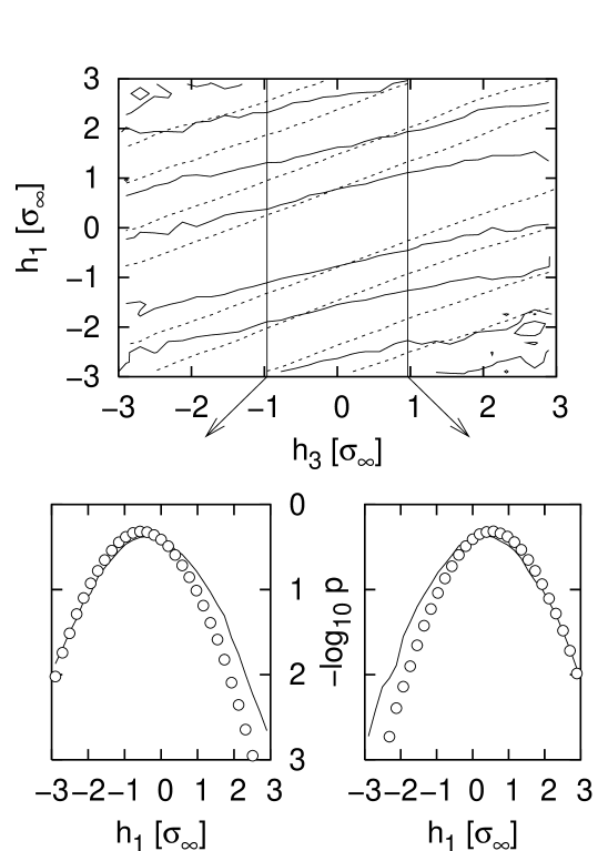
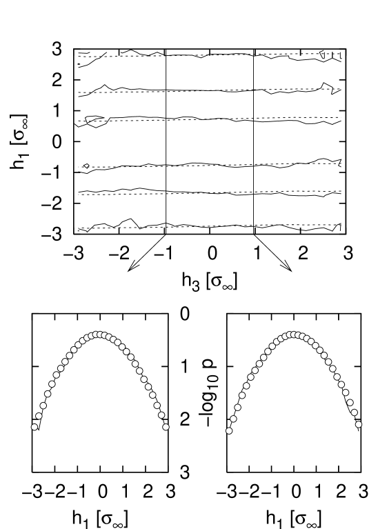
Figure 14: A check of the Chapman-Kolmogorov equation (21) for the Au surface for two different scale separations $\Delta r=14$$\,\mathrm{nm}$ (a) and 35$\,\mathrm{nm}$ (b). In both cases $r_{2}=169$$\,\mathrm{nm}$. The plots are organized in the same way as fig. 12. The pdf representing the left side of (21) are shown with solid lines, the integrated pdf of the right side of (21) as dashed lines and circles.

A third method which we did not use here but which is reported in the literature is based on the description of the stochastic process by a Langevin equation. With this knowledge of the Langevin equation (11) the noise can be reconstructed and analyzed with respect to its correlation Siefert2003 ; Marcq2001 .

5.2 Conclusions on Markov properties

The results of the methods described above were combined to determine whether Markov properties of the height increment $h_{r}(x)$ in the scale variable are present for our surface measurements. We found Markov properties for all the selected examples of surface measurement data.

Surface	$l_{M}$	Surface	$l_{M}$	Surface	$l_{M}$
Road 1	33$\,\mathrm{mm}$	Road 2	10$\,\mathrm{mm}$	Road 3	4.2$\,\mathrm{mm}$
Road 4	17$\,\mathrm{mm}$	Road 5	4.2$\,\mathrm{mm}$	Au	25$\,\mathrm{nm}$
Crack	20$\,\mathrm{\mu m}$

Table 1: Markov lengths $l_{M}$ for all the surfaces presented.

It is also common to all examples that these Markov properties are not universal for all scale separations $\Delta r$ but there exists a lower threshold which we call the Markov length $l_{M}$. It was determined in each case by systematic application of the three testing procedures for all accessible length scales $r$ and scale separations $\Delta r$. The resulting values are listed in table 1. The presence of Markov properties only for values of $\Delta r$ above a certain threshold has also been found for stochastic data generated by a large variety of processes and especially occurs in turbulent velocities Friedrich1998a ; Friedrich1998b ; Friedrich2000b ; Renner2001 ; Ghasemi2003 .

The meaning of this Markov length $l_{M}$ may be seen in comparison with a mean free path length of a Brownian motion. Only above this mean free path is a stochastic process description valid. For smaller scales there must be some coherence which prohibits a description of the structure by a Markov process. If for example the description of a surface structure requires a second order derivative in space, a Langevin equation description (11) becomes impossible. In this case a higher dimensional Langevin equation (at least two variables) is needed. It may be interesting to note that the Markov length we found for the Au surface of about 30$\,\mathrm{nm}$ coincides quite well with the size of the largest grain structures we see in fig. 5. Thus the Au surface may be thought of as a composition of grains (coherent structures) by a stochastic Markov process.

In the case of Road 2 with its strong periodicity at 0.2$\,\mathrm{m}$ the Markov properties end slightly above this length scale. It seems evident that here the Markov property is destroyed by the periodicity. While some of the other surfaces also have periodicities, these are never as sharp as for Road 2. An upper limit for Markov properties could not be found for any of the other surfaces.

Another interesting finding can be seen from figs. 2, 6, 8, and 10. There is no connection between the scaling range and the range where Markov properties hold. Regimes of scaling and Markov properties are found to be distinct, overlapping or covering, depending on the surface. Data sets which fulfill the Markov property do not in all cases show a scaling regime at all. Also, on the other hand, scaling features seem not to imply Markov properties, which has been indicated previously for some numerically generated data in Friedrich1998a . While there is always an upper limit of the scaling regime, we found only one surface for which the Markov properties possess an upper limit.

6 Estimation of drift and diffusion coefficients

As a next step we want to concentrate on extracting the concrete form of the stochastic process, if the Markov properties are fulfilled. As mentioned in section 2 our analysis is based on the estimation of Kramers-Moyal coefficients. The procedure we use to obtain the drift ($D^{(1)}$) and diffusion coefficient ($D^{(2)}$) for the Fokker-Planck equation (2) was already outlined by Kolmogorov Kolmogorov1931 , see also Risken1984 ; Renner2001 . First, the conditional moments $M^{(k)}(h_{r},r,\Delta r)$ for finite step sizes $\Delta r$ are estimated from the data via the moments of the conditional probabilities. This is done by application of the definition in eq. (8), which is recalled here:

$$M^{(k)}(h_{r},r,\Delta r)=\frac{r}{k!\Delta r}\int_{\scriptscriptstyle-\infty}^{\scriptscriptstyle+\infty}(\tilde{h}-h_{r})^{k}\;p(\tilde{h},r-\Delta r|h_{r},r)\;d\tilde{h}$$ (22)

The conditional probabilities in the integral are obtained by counting events in the measurement data as shown already in section 5. Here, one fundamental difficulty of the method arises: For reliable estimates of conditional probabilities we need a sufficient number of events even for rare combinations of $\tilde{h},h_{r}$. Consequently, a large amount of data points is needed. This problem becomes even more important if one takes into account that a large range in $r$ should be considered. The number of statistically independent intervals $h_{r}$ is limited by the length of the given data set and decreases with increasing $r$.

In a second step, the coefficients $D^{(k)}(h_{r},r)$ are obtained from the limit of $M^{(k)}(h_{r},r,\Delta_{r})$ when $\Delta r$ approaches zero (see definition in eq. (7)). For fixed values of $r$ and $h_{r}$ a straight line is fitted to the sequence of $M^{(k)}(h_{r},r,\Delta r)$ depending on $\Delta r$ and extrapolated against $\Delta r=0$. The linear dependence corresponds to the lowest order term when the $\Delta r$-dependence of $M^{(k)}(h_{r},r,\Delta r)$ is expanded into a Taylor series for a given Fokker-Planck equation Friedrich2002 ; Siefert2003 . Our interpretation is that this way of estimating the $D^{(k)}$ is the most advanced one, and also performs better than first parameterizing the $M^{k}$ and then estimating the limit $\Delta r\rightarrow 0$ for this parameterization, as previously suggested in Renner2001 ; Renner2001Diss .

There have been suggestions to fit functions to $M^{(k)}$ other than a straight line, especially for the estimation of $D^{(2)}$, see Renner2001Diss . Furthermore it has been proposed to use particular terms of the above-mentioned expansion to directly estimate $D^{(k)}(h_{r},r)$ without extrapolation Ragwitz2001 . On the other hand, in Sura2002 it becomes clear that there can be manifold dependences of $M^{(k)}$ on $\Delta r$ which in general are not known for a measured data set. Consequently, one may state that there is still a demand to improve the estimation of $D^{(k)}$. At the present time we suggest to show the quality of the estimated $D^{(k)}$ by verification of the resulting Fokker-Planck equation, once its drift and diffusion coefficients have been estimated. However, for our data neither nonlinear fitting functions nor correction terms applied to the $M^{(k)}$ resulted in improvements of the estimated $D^{(k)}$.

A crucial point in our estimation procedure is the range of $\Delta r$ where the fit can be performed. Only those $\Delta r$ can be used where Markov properties were found in the scale domain. In section 5 we showed that for our data Markov properties are given for $\Delta r$ larger than the Markov length $l_{M}$ (see table 1). In order to reduce uncertainty, a large range of $\Delta r$ as the basis of the extrapolation is desirable. From eq. (22) it can be seen, however, that $\Delta r$ must be smaller than $r$. As a compromise between accuracy and extending the scale $r$ to smaller values, in many cases an extrapolation range of $l_{M}\leq\Delta r\leq 2\,l_{M}$ was used (cf. table 2). This procedure is shown in fig. 15 for Road 1.

Surface	$l_{M}$	$l_{\mathit{max}}$	Surface	$l_{M}$	$l_{\mathit{max}}$
Road 1	33$\,\mathrm{mm}$	67$\,\mathrm{mm}$	Road 2	10$\,\mathrm{mm}$	21$\,\mathrm{mm}$
Road 3	4.2$\,\mathrm{mm}$	19$\,\mathrm{mm}$	Road 4	17$\,\mathrm{mm}$	25$\,\mathrm{mm}$
Road 5	4.2$\,\mathrm{mm}$	8.3$\,\mathrm{mm}$	Au	25$\,\mathrm{nm}$	84$\,\mathrm{nm}$
Crack	20$\,\mathrm{\mu m}$	44$\,\mathrm{\mu m}$

Table 2: Extrapolation ranges for all the presented surfaces. Listed are the smallest ($l_{M}$) and largest ($l_{\mathit{max}}$) values of $\Delta r$ used for extrapolation of the $D^{(k)}(h_{r},r)$.

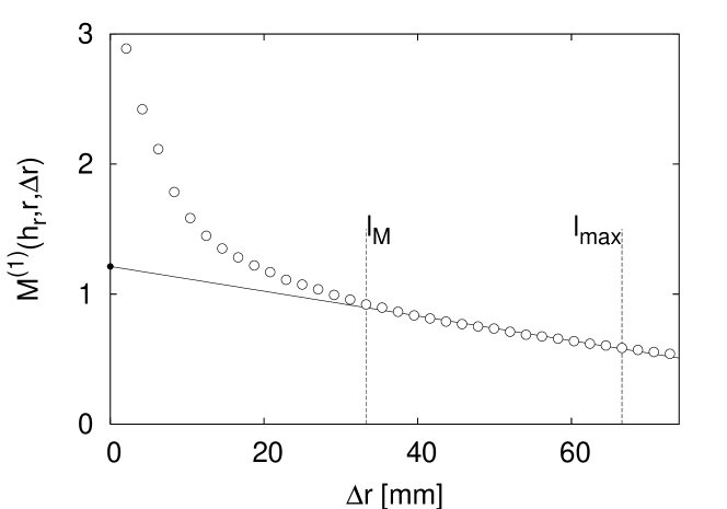
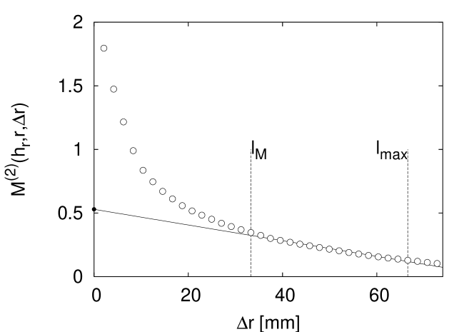
Figure 15: Extrapolation procedure for $D^{(1)}$ (a) and $D^{(2)}$ (b), illustrated for surface Road 1. Length scale $r$ is 108$\,\mathrm{mm}$, $h_{r}$ is $-\sigma_{\infty}$. Values of $M^{(1)}$ and $M^{(2)}$ inside the range marked by broken lines were used for the extrapolation. The results $D^{(1)}(h_{r},r)$ and $D^{(2)}(h_{r},r)$ are marked with filled circles on the vertical axis.

6.1 Estimation results

Following the procedure outlined above, $D^{(1)}(h_{r},r)$ and $D^{(2)}(h_{r},r)$ were derived for the measurement data presented in section 3, with the exception of Road 5 (see below). For the road surfaces, estimations were performed for length scales $r$ separated by ten measurement steps or 10.4$\,\mathrm{mm}$, respectively, to reach a sufficient density over the range where the coefficients were accessible. Figures 16 and 17 show estimations of the drift coefficients $D^{(1)}$ and the diffusion coefficients $D^{(2)}$ for the road surfaces, each performed for one fixed length scale $r$. The error bars are estimated from the errors of $M^{(k)}(h_{r},r,\Delta r)$ via the number of statistically independent events contributing to each value, assuming that each bin of $p(h_{1},r_{1}|h_{0},r_{0})$ containing $N$ events has an intrinsic uncertainty of $\pm\sqrt{N}$. Additionally, values of $D^{(4)}$ are added to the plots of $D^{(2)}$ which have been estimated in the same way. Thus it can be seen that in all cases $D^{(4)}$ is small compared to $D^{(2)}$, except for Road 4, and in most cases its statistical errors are larger than the values themselves. Negative values are not shown because the vertical axes start at zero. As $M^{(4)}$ is positive by definition, the occurence of negative values of $D^{(4)}$ results from the limit $\Delta r\rightarrow 0$ and should be only due to the statistical errors involved. Even if there is no evidence that $D^{(4)}$ is identically zero, the presented values give a hint that its influence in the Kramers-Moyal expansion (6) is rather small and the assumption of a Fokker-Planck equation (2) is justifiable, with the possible exception of Road 4.

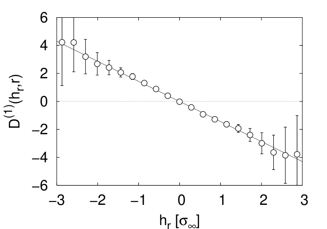
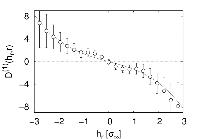
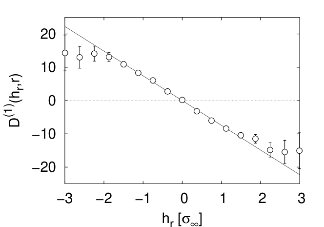
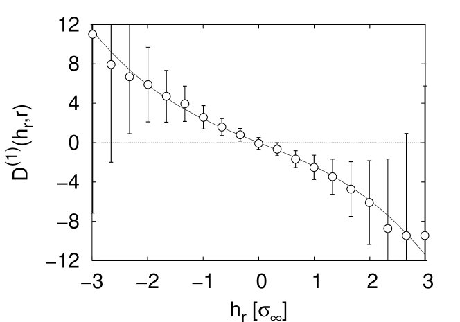
Figure 16: Estimated drift coefficients $D^{(1)}(h_{r},r)$ of the Fokker-Planck equation for the road surfaces shown in fig. 1. Scales $r$ are 108$\,\mathrm{mm}$ (Road 1), 114$\,\mathrm{mm}$ (Road 2), 94$\,\mathrm{mm}$ (Road 3), and 104$\,\mathrm{mm}$ (Road 4). Parameterizations are shown as lines.

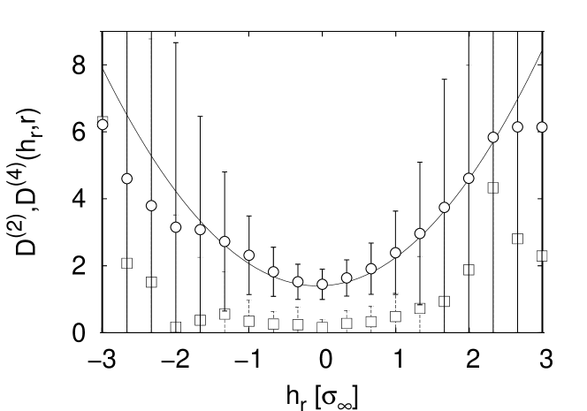
Figure 17: Estimated diffusion coefficients $D^{(2)}(h_{r},r)$ (circles) of the Fokker-Planck equation for road surfaces shown in fig. 1. Additionally the fourth Kramers-Moyal coefficients $D^{(4)}(h_{r},r)$ are shown as squares. Scales $r$ are as in fig. 16. Parameterizations are shown as lines.

Estimated drift and diffusion coefficients $D^{(1)}$ and $D^{(2)}$ for the Au surface are shown in fig. 18 for $r=169$$\,\mathrm{nm}$. Again, $D^{(4)}$ was added to the plot of $D^{(2)}$, in this case without error bars to enhance clarity. Errors of $D^{(4)}$ are in this case always much larger than the values themselves and would cover the values of $D^{(2)}$ as well as their errors. Also the error bars of $D^{(2)}$ appear to be quite large for the Au surface. The data here are measured as two-dimensional images, thus the number of statistically independent $h_{r}(x)$ decreases quadratically with increasing $r$, resulting in rather large error estimates. For the calculation of $D^{(k)}$ nevertheless all accessible $h_{r}(x)$ were used. As the regime of Markov properties starts at $\Delta r=25\,\mathrm{nm}$, the range $25\,\mathrm{nm}\leq\Delta r\leq 84\,\mathrm{nm}$ was used as basis for the extrapolation (see table 2). For $r<84\,\mathrm{nm}$ the upper limit was reduced in order to derive the coefficients also for smaller scales $r$ (compare also section 6). In this way the drift and diffusion coefficients of the Au film could be worked out from 281 down to 56$\,\mathrm{nm}$.

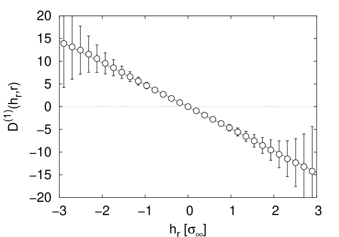
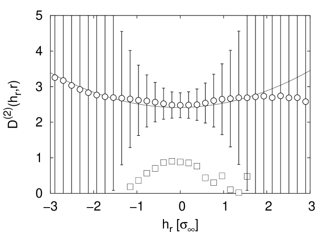
Figure 18: Estimated drift (a) and diffusion (b) coefficient of the Au surface for $r=169$$\,\mathrm{nm}$. Estimates of $D^{(4)}$ are added as squares in (b).

In the same way as for the other surfaces, estimations of the Kramers-Moyal coefficients were performed for the steel crack. The results are shown in fig. 19. Again, the estimates for $D^{(4)}$ are also presented, which are of the same order of magnitude as $D^{(2)}$ for higher values of $h_{r}$ ($|h_{r}|>0.5\sigma_{\infty}$).

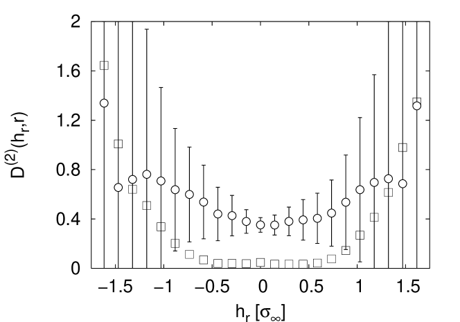
Figure 19: Estimated Kramers-Moyal coefficients for surface Crack for a length scale $r=49$$\,\mathrm{\mu m}$. (a) $D^{(1)}(h_{r},r)$, (b) $D^{(2)}(h_{r},r)$ and $D^{(4)}(h_{r},r)$.

For the surface Road 5 (cf. fig. 8) drift and diffusion coefficients could not be estimated. The reason can be seen in fig. 20. The diagram shows the dependence of $M^{(1)}(h_{r},r,\Delta_{r})$ and $M^{(2)}(h_{r},r,\Delta r)$ on $\Delta r$ for fixed $r$ and $h_{r}$, in this case 104$\,\mathrm{mm}$ and $-0.6\sigma_{\infty}$. For $\Delta r>l_{M}$ it can be seen that $M^{(1)}$ and $M^{(2)}$ behave like $1/\Delta r$. This behaviour can be explained by the presence of some additional uncorrelated noise, where additional means independent of the stochastic process. A similar behaviour was found for financial market data Renner2001b . In this case the integral in eq. (22) will tend to a constant for small $\Delta r$, independent of the value of $\Delta r$. Because we divide the integral by $\Delta r$, the $M^{(k)}$ will then diverge as $\Delta r$ approaches zero. Note that within the same mathematical framework the presence of uncorrelated noise can be quantitatively determined Siefert2003 .

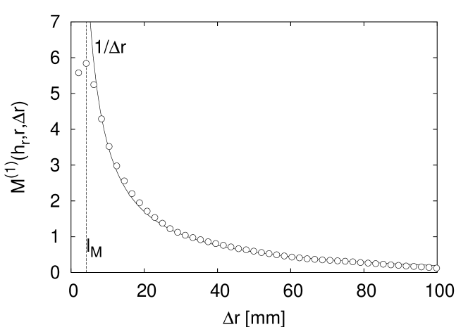
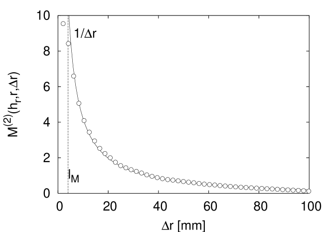
Figure 20: Uncorrelated noise in the case of surface Road 5. Dependence of (a) $M^{(1)}(h_{r},r,\Delta r)$ and (b) $M^{(2)}(h_{r},r,\Delta r)$ on $\Delta r$ for $r=104\,\mathrm{mm}$ and $h_{r}=-0.6\sigma_{\infty}$. The Markov length $l_{M}$ is marked with a dashed line. For illustration a function proportional to $1/\Delta r$ is fitted to the $M^{(k)}$.

6.2 Conclusions on the estimation of drift and diffusion coefficients

Estimations of the drift and diffusion coefficients $D^{(1)}(h_{r},r)$ and $D^{(2)}(h_{r},r)$ have been performed for all the surfaces introduced in section 3. An exception is Road 5, where the stochastic process in the scale variable, while still Markovian, appears to be dominated by additional uncorrelated noise. From eqs. (7) and (8) it can be seen that this leads to diverging Kramers-Moyal coefficients $D^{(k)}$, as is the case for Road 5.

As mentioned above, the magnitude of the fourth Kramers-Moyal coefficient $D^{(4)}$ is of particular importance. If $D^{(4)}$ can be taken as zero, the whole scale dependent complexity can be described by a Fokker-Planck equation. Otherwise, if $D^{(4)}$ is not zero, an infinite set of $D^{(k)}$ is necessary. In terms of a Langevin equation (11), for $D^{(4)}\neq 0$ no Gaussian noise is present. This case is related to unsteady stochastic processes Honerkamp1990 . As we see from the topographies in figs. 1 and 9, jumps are more likely to be present for the Road 4 and Crack surfaces than for the remaining ones. This impression is consistent with the result that here we find $D^{(4)}\neq 0$. As a consequence, in these cases the Fokker-Planck equation with a drift and diffusion coefficient is not sufficient to describe the stochastic process in the scale variable, because the higher coefficients cannot be neglected. The reconstruction of conditional probabilities (cf. section 7) failed for these surfaces.

The range of scales where the drift and diffusion coefficients could be estimated varies for the different surfaces, depending on the Markov length on one side and on the length of the measured profiles on the other side. In the case of Road 2 an additional upper limit for the Markov properties was caused by the influence of a strong periodicity of the pavement.

7 Verification of the estimated Fokker-Planck equations

In the previous section methods to estimate the Kramers-Moyal coefficients were discussed. We found that this estimation is not trivial. To prove the quality of the estimated $D^{(k)}$ we now want to verify the corresponding Fokker-Planck equations.

7.1 Parameterization of Drift and Diffusion Coefficients

With the estimations of the drift and diffusion coefficient from section 6 for each surface a Fokker-Planck equation (2) is defined which should describe the corresponding process. For the verification of these coefficients it is additionally desirable to generate parameterizations which define $D^{(1)}(h_{r},r)$ and $D^{(2)}(h_{r},r)$ not only at discrete values but at arbitrary points in the $(h_{r},r)$-plane.

Such parameterizations have already been shown in figs. 16, 17, 18, and 19, as lines together with the estimated discrete values. For $D^{(1)}$ it can be seen that for all surfaces a straight line with negative slope was used, with additional cubic terms for Road 2, Road 4, and Crack. The diffusion coefficients were in all cases parameterized as parabolic functions. The special shape of the diffusion coefficient for Road 2 was parameterized as one inner and one outer parabola for small and larger values of $h_{r}$, respectively (compare with fig. 17). We would like to note that both the drift and diffusion coefficients of the cobblestone road presented in Waechter2003_plus_preprint are best fitted by piecewise linear functions with steeper slopes for larger $h_{r}$.

It is easy to verify that with a linear $D^{(1)}$ and a constant $D^{(2)}$ the Fokker-Planck equation (2) describes a Gaussian process, while with a parabolic $D^{(2)}$ the distributions become non-Gaussian, also called intermittent or heavy tailed. For the Au surface it can be seen in fig. 18 that $D^{(2)}$ has only a weak quadratic dependence on $h_{r}$ and possibly could also be interpreted as constant (we nevertheless kept the small quadratic term because it is confirmed by the verification procedure below). If $D^{(2)}$ is constant in $h_{r}$ the type of noise in the corresponding Langevin equation (11) is no longer multiplicative but additive, which results in Gaussian noise in the process. Thus the statistics of $h_{r}$ in $r$ will always stay Gaussian, and all moments $\langle h_{r}^{n}\rangle$ with $n>2$ can be expressed by the first and second one. As a further consequence, the scaling exponents $\xi_{n}$ (see section 4) are obtained by $\langle h_{r}^{n}\rangle\sim\langle h_{r}^{2}\rangle^{n/2}$ as $\xi^{n}=\frac{n}{2}\xi_{2}$. This linear dependence on $n$ denotes self-affinity rather than multi-affinity and is confirmed by the scaling analysis in section 4.1.

7.2 Reconstruction of empirical pdf

Next, we want to actually evaluate the precision of our results. Therefore we return to eq. (2). Knowing $D^{(1)}$ and $D^{(2)}$ it should be possible to calculate the pdf of $h_{r}$ with the corresponding Fokker-Planck equation. Equation (2) can be integrated over $h_{0}$ and is then valid also for the unconditional pdf:

$$-r\,\frac{\partial}{\partial r}\;p(h_{r},r)\,=$$

$$\left\{-\frac{\partial}{\partial h_{r}}D^{(1)}(h_{r},r)+\frac{\partial^{2}}{\partial h_{r}^{2}}D^{(2)}(h_{r},r)\right\}\,p(h_{r},r)$$

Now at the largest scale $r_{0}$ where the drift and diffusion coefficients could be worked out the empirical pdf is parameterized and used as the initial condition for a numerical solution of eq. (7.2). For several values of $r$ the reconstructed pdf is compared to the respective empirical pdf, as shown below in this section. If our Fokker-Planck equation successfully reproduces these single scale pdf, the structure functions $\langle h_{r}^{n}\rangle$ can also easily be obtained.

A second verification is the reconstruction of the conditional pdf by a numerical solution of Fokker-Planck equation (2) for the conditional pdf. Reconstructing the conditional pdf this way is much more sensitive to deviations in $D^{(1)}$ and $D^{(2)}$. This becomes evident by the fact that the conditional pdf (and not the unconditional pdf of figs. 21 and 23) determine $D^{(1)}$ and $D^{(2)}$ and thus the stochastic process, see eqs. (7) and (8). The knowledge of the conditional pdf also gives access to the complete $n$-scale joint pdf (eq. 4). Here again the difference from the multiscaling analysis becomes clear, which analyses higher moments $\langle h_{r}^{n}\rangle=\int h_{r}^{n}\cdot p(h_{r})\,\mathrm{d}h_{r}$ of $h_{r}$, and does not depend on the conditional pdf. It is easy to show that there are many different stochastic processes which lead to the same single scale pdf $p(h_{r})$.

For both verification procedures we use a technique which is mentioned in Risken1984 and has already been used in Renner2001 ; Waechter2003_plus_preprint . An approximative solution of the Fokker-Planck eq. (2) for infinitesimally small steps $\Delta r$ over which $D^{(k)}$ can be taken as constant in $r$, is known Risken1984

$$p(h_{1},r-\Delta r|h_{0},r)=\frac{1}{2\sqrt{\pi D^{(2)}(h_{r},r)\Delta r}}$$ (24)

$$\times\exp{\left(-\frac{(h_{1}-h_{0}-D^{(1)}(h_{0},r)\Delta r)^{2}}{4D^{(2)}(h_{r},r)\Delta r}\right)}\,.$$

A necessary condition for a Markov process is the validity of the Chapman-Kolmogorov equation (21) Risken1984 , which allows to combine two conditional pdf with adjacent intervals in $r$ into one conditional pdf spanning the sum of both intervals. By an iterative application of these two relations we are able to obtain conditional probabilities $p(h_{i},r_{0}-i\Delta r|h_{0},r_{0})$ spanning large intervals in the scale $r$, given that for all involved scales $r_{i}$ the drift and diffusion coefficients are known.

In the following the results of this verification procedure are shown for those surfaces where the drift and diffusion coefficients of the Fokker-Planck equation could be obtained.

7.3 Verification results

The results of the reconstruction of the unconditional pdf for the road surfaces with scaling properties are presented in fig. 21. The pdf of Road 1 show at smaller scales a peak around 5$\,\mathrm{\sigma_{\infty}}$ which is not reproduced by our Fokker-Planck equation because in this regime of $h_{r}$ $D^{(1)}$ and $D^{(2)}$ could not be estimated with sufficient precision. Here it has to be noted that according to eq. (12) $\sigma_{\infty}>\sigma_{r}$ for any $r$, and thus 5$\,\mathrm{\sigma_{\infty}}$ is a large value for a pdf, denoting quite rare events (the $r$-dependence of $\sigma_{r}$ has been presented by $S^{2}(r)=\sigma_{r}^{2}$, see section 4). The magnitudes of the estimated drift and diffusion coefficients had to be adjusted by a factor of 0.65 to give optimal results in the reconstruction. For Road 2 it is likely that the correspondence between the emprical and reconstructed pdf could be improved by a more advanced parameterization of the nontrivial shape especially of the estimated drift coefficient (see fig. 16). Here, the estimated drift and diffusion coefficients could be used without adjustment. The reconstructed pdf for Road 3 are in perfect agreement with the empirical ones. A substantial adjustment factor of 0.20 for $D^{(1)}$ and 0.26 for $D^{(2)}$ was necessary to achieve the best result.

Figure 21: Numerical solution of the Fokker-Planck equation (7.2) compared to the empirical pdf (symbols) for road surfaces with scaling properties. For each surface, the topmost solid line corresponds to an empirical pdf parameterized at the largest scale, and the dashed lines to the reconstructed pdf. Scales are (from top to bottom) for Road 1: 316, 158, 79, 66$\,\mathrm{mm}$, for Road 2: 158, 79, 47, 20$\,\mathrm{mm}$, for Road 3: 188, 95, 47, 24$\,\mathrm{mm}$. Pdf are shifted in the vertical direction for clarity of presentation.

Reconstructed conditional pdf are shown in fig. 22 for the road surfaces. While there are deviations for larger values of $h_{0},h_{1}$, the overall agreement between the empirical and reconstructed pdf is good. Especially the rather complicated shape of the conditional pdf of Road 2 appears to be well modelled by our coefficients $D^{(1)},D^{(2)}$. As mentioned above, an improved parameterization of $D^{(1)}$ may lead to even better results. The magnitudes of $D^{(1)},D^{(2)}$ were adjusted by the same factors as for the unconditional pdf above.

Figure 22: Numerical solution of the Fokker-Planck equation (2) compared to the empirical pdf for road surfaces with scaling properties. Similar to fig. 12 in each case a contour plot of empirical (solid lines) and reconstructed pdf (broken lines) is shown on top, with contour levels as in fig. 12. Below two cuts at $h_{0}\approx\pm\sigma_{\infty}$ are located. Here, empirical pdf are plotted as symbols. Scales are $r_{0}=304\,\mathrm{mm}$, $r_{1}=158\,\mathrm{mm}$ (Road 1), $r_{0}=158\,\mathrm{mm}$, $r_{1}=112\,\mathrm{mm}$ (Road 2), and $r_{0}=188\,\mathrm{mm}$, $r_{1}=92\,\mathrm{mm}$ (Road 3).

Figure 23: Numerical solutions of the Fokker-Planck equations (2) and (7.2) compared to the empirical pdf for the Au surface.
(a) Results of the integrated equation (7.2) presented as in fig. 21. Scales $r$ are 281, 246, 148, and 56$\,\mathrm{nm}$ (from top to bottom).
(b), (c) Numerical solution of equation (2) for the conditional pdf compared to the empirical pdf at scales $r_{0}=183\,\mathrm{nm}$, $r_{1}=155\,\mathrm{nm}$ (b) and $r_{0}=281\,\mathrm{nm}$, $r_{1}=56\,\mathrm{nm}$ (c). The organisation of the diagram is as in fig. 22.

In the case of the Au film the drift and diffusion coefficients could be worked out from 281 down to 56$\,\mathrm{nm}$, see section 6. In contrast to this regime, the range of correlation between scales is only about 40$\,\mathrm{nm}$, i.e., height increments on scales which are separated by at least 40$\,\mathrm{nm}$ are uncorrelated. Nevertheless, both verification procedures outlined in section 7 gave good results over the whole range from 281 to 56$\,\mathrm{nm}$ as shown in fig. 23. Here the estimated $D^{(1)}$ and $D^{(2)}(h_{r},r)$ were multiplied by factors 1.3 and 2.2, respectively.

7.4 Discussion of the verification procedure

For the verification of the drift and diffusion coefficients estimated in section 6 numerical solutions of the Fokker-Planck equations (2) and (7.2) have been performed using these estimations. The reconstructed pdf have been compared to the empirical ones to validate the descripition of the data sets as realizations of stochastic processes obeying the corresponding Fokker-Planck equation.

Good results were obtained for most surfaces where the drift and diffusion coefficients could be derived. In the case of Road 4 and Crack we found that the higher Kramers-Moyal coefficients $D^{(3)}$ and $D^{(4)}$ were significantly different from zero, and the empirical pdf could not be reproduced with a Fokker-Planck equation (which only uses $D^{(1)}$ and $D^{(2)}$).

It may be surprising that the correspondence between the empirical and reconstructed pdf seems better for the conditional rather than for the unconditional pdf in some cases (compare figs. 21 and 22). One reason may be that in fig. 22 it is clear that the empirical pdf are not precisely defined for combinations of large $h_{0}$ and $h_{1}$. The eye concentrates on the central regions of the contour plots where the uncertainty of the empirical pdf is reduced, as well as deviations due to possible inaccuracies and uncertainties of our drift and diffusion coefficients. This effect is also confirmed by our mathematical framework where all steps in the procedure are based on the estimation and evaluation of the conditional (not the unconditional) pdf.

The reconstruction procedure allows also to adjust the estimated coefficients in order to improve the above-mentioned description, thus compensating for a number of uncertainties in the estimation process. While the functional form of $D^{(1)}$ and $D^{(2)}$ found in section 6 for all surfaces could be confirmed, in most cases the magnitudes of the estimated values had to be adjusted to give satisfactory results in this reconstruction procedure. We found this effect also when analysing turbulent velocities and financial data. One reason may be the uncertainties of the estimation procedure. A second source of deviations may be that the dependence of $M^{(k)}(h_{r},r,\Delta r)$ on $\Delta r$ is not always purely linear in the extrapolation range (see section 6). Thus fitting a straight line and extrapolating against $\Delta r=0$ may lead to coefficients $D^{(1)}$ and $D^{(2)}$ which still have the correct functional form in $h_{r}$ but incorrect magnitudes. As mentioned in section 6, in our case no general improvements could be achieved by the use of nonlinear (i.e. polynomial) fitting functions or higher order terms of the corresponding Taylor expansion. It is possible that the range of $\Delta r<l_{M}$ where no Markov properties are given is in most cases large enough that approximations for small $\Delta r$ are inaccurate. We would like to note that there are also data sets which did not require any adjustment of the estimated coefficients, see Road 2 and Waechter2003_plus_preprint . A last remark concerns the latest results in the case of Road 1, see fig. 15. If the fraction of $M^{(k)}(\Delta r)$ which is proportional to $1/\Delta r$ is substracted before performing the extrapolation, the resulting $D^{(k)}$ are substantially improved in their magnitudes. This may be a way to correct the extrapolation of the $D^{(k)}$ in cases where uncorrelated noise is involved.

In any case, whether an adjustment of $D^{(1)}$ and $D^{(2)}$ was needed or not, for the presented surfaces a Fokker-Planck equation was found which reproduces the conditional pdf. Together with the verification of the Markov property (4) thus a complete description of the $n$-scale joint pdf is given, which was the aim of our work.

8 Conclusions

For the analysis and characterization of surface roughness we have presented a new approach and applied it to different examples of rough surfaces. The objective of the method is the estimation of a Fokker-Planck equation (2) which describes the statistics of the height increment $h_{r}(x)$ in the scale variable $r$. A complete characterization of the corresponding stochastic process in the sense of multiscale conditional probabilities is the result.

The application to different examples of surface measurement data showed that this approach cannot serve as a universal tool for any surface, as it is also the case for other methods like those based on self- and multi-affinity. With given conditions, namely the Markov property and a vanishing fourth order Kramers-Moyal coefficient (cf. section 2), a comprehensive characterization of a single surface is obtained. The features of the scaling analysis are included, and beyond that a deeper insight in the complexity of roughness is achieved. As shown in Jafari2003 such knowledge about a surface allows the numerical generation of surface structures which should have the same complexity. This may be of high interest for many research fields based on numerical modelling.

The precise estimation of the magnitudes of the drift and diffusion coefficients for surface measurement data still remains an open problem. While for other applications a number of approaches have been developed Renner2001 ; Friedrich2002 ; Ragwitz2001 ; Sura2002 in any case a verification of the estimated Fokker-Planck equation is necessary and may lead to significant adjustments, as it is the case for some of our data sets.

- (1) R. S. Sayles and T. R. Thomas. Surface topography as a nonstationary random process. Nature, 271:431–434, 1978.
- (2) Tamas Vicsek. Fractal Growth Phenomena. World Scientific, Singapore, 2nd edition, 1992.
- (3) Albert-László Barabási and H. Eugene Stanley. Fractal concepts in surface growth. Cambridge University Press, Cambridge, 1995.
- (4) Steve Davies and Peter Hall. Fractal analysis of surface roughness by using spatial data. Journal of the Royal Statistical Society B, 61(1):3–37, 1999.
- (5) Ulrich Wendt, Katharina Stiebe-Lange, and M. Smid. On the influence of imaging conditions and algorithms on the quantification of surface topography. Journal of Microscopy, 207:169–179, 2002.
- (6) C. V. Dharmadhikari, R. B. Kshirsagar, and S. V. Ghaisas. Scaling behaviour of polished surfaces. Europhysics Letters, 45(2):215–221, 1999.
- (7) M. Saitou, M. Hokama, and W. Oshikawa. Scaling behaviour of polished (110) single crystal nickel surfaces. Applied Surface Science, 185(1-2):79–83, 2001.
- (8) Uwe Sydow, M. Buhlert, and P. J. Plath. Characterization of electropolished metal surfaces. Accepted for Discrete Dynamics in Nature and Society, 2003.
- (9) Jens Feder. Fractals. Plenum Press, New York, London, 1988.
- (10) Fereydoon Family and T. Vicsek, editors. Dynamics of fractal surfaces. World Scientific, Singapore, 1991.
- (11) Rudolf Friedrich, Thomas Galla, Antoine Naert, Joachim Peinke, and Th. Schimmel. Disordered structures analysed by the theory of Markov processes. In Jürgen Parisi, St. C. Müller, and W. Zimmermann, editors, A Perspective Look at Nonlinear Media, volume 503 of Lecture Notes in Physics, pages 313–326. Springer Verlag, Berlin, 1998.
- (12) Matthias Waechter, Falk Riess, Holger Kantz, and Joachim Peinke. Stochastic analysis of surface roughness. Europhysics Letters, 64(5):579–585, 2003. See also preprints arxiv:physics/0203068 and arxiv:physics/0310159.
- (13) G. R. Jafari, S. M. Fazeli, F. Ghasemi, S. M. Vaez Allaei, M. Reza Rahimi Tabar, A. Iraji Zad, and G. Kavei. Stochastic analysis and regeneration of rough surfaces. Physical Review Letters, 91(22):226101, 2003.
- (14) Christoph Renner, Joachim Peinke, and Rudolf Friedrich. Experimental indications for Markov properties of small-scale turbulence. Journal of Fluid Mechanics, 433:383–409, 2001.
- (15) Stephan Lueck, Joachim Peinke, and Rudolf Friedrich. Experimental evidence of a phase transition to fully developed turbulence in a wake flow. Physical Review Letters, 83(26):5495–5498, 1999.
- (16) Rudolf Friedrich, Joachim Peinke, and Christoph Renner. How to quantify deterministic and random influences on the statistics of the foreign exchange markets. Physical Review Letters, 84(22):5224–5227, 2000.
- (17) Marcel Ausloos and K. Ivanova. Dynamical model and nonextensive statistical mechanics of a market index on large time windows. Physical Review E, 68(4):046122, 2003.
- (18) F. Ghasemi, A. Bahraminasab, S. Rahvar, and M. Reza Rahimi Tabar. Stochastic nature of cosmic microwave background radiation. Preprint arxiv:astro-phy/0312227, 2003.
- (19) Please note that there have been different definitions of increments, especially the left-justified increment . Here we use the symmetrical increment in order to avoid the introduction of spurious correlations between scales Waechter2004a .
- (20) Maria Haase, 2003. Private communication.
- (21) Christoph Renner. Markovanalysen stochastisch fluktuierender Zeitserien. PhD thesis, Carl-von-Ossietzky University, Oldenburg, Germany, 2001. http://docserver.bis.uni-oldenburg.de/publikationen/dissertation/2002/r%enmar02/renmar02.html.
- (22) Hannes Risken. The Fokker-Planck equation. Springer, Berlin, 1984.
- (23) In contrast to other applications (like financial data), in this case the process direction from large to smaller scales is unimportant and was chosen arbitrarily. When the process direction is reversed, the coefficients change only slightly, preserving both the form and behaviour of the Fokker-Planck equation. The logarithmic variable was used in order to preserve consistency, see Renner2001 ; Friedrich1998a ; Friedrich2000a .
- (24) Andrej N. Kolmogorov. Über die analytischen Methoden in der Wahrscheinlichkeitsrechnung. Mathematische Annalen, 104:415–458, 1931.
- (25) Matthias Waechter, Falk Riess, and Norbert Zacharias. A multibody model for the simulation of bicycle suspension systems. Vehicle System Dynamics, 37(1):3–28, 2002.
- (26) R. Benzi, S. Ciliberto, R. Tripiccione, C. Baudet, F. Massaioli, and S. Succi. Extended self-similarity in turbulent flows. Physical Review E, 48(1):29, 1993.
- (27) Markus Alber and Joachim Peinke. An improved multifractal box-counting algorithm, virtual phase transition, and negative dimensions. Physical Review E, 57:5489, 1998.
- (28) Rudolf Friedrich, J. Zeller, and Joachim Peinke. A note in three point statistics of velocity increments in turbulence. Europhysics Letters, 41:153, 1998.
- (29) I. N. Bronstein and K. A. Semendjajew. Taschenbuch der Mathematik. Teubner, Stuttgart, 1991.
- (30) Rudolf Friedrich and Joachim Peinke. Statistical properties of a turbulent cascade. Physica D, 102:147, 1997.
- (31) Rudolf Friedrich and Joachim Peinke. Description of a turbulent cascade by a Fokker-Planck equation. Physical Review Letters, 78:863, 1997.
- (32) Mario Ragwitz and Holger Kantz. Indispensable finite time corrections for Fokker-Planck equations from time series data. Physical Review Letters, 87:254501, 2001.
- (33) Malte Siefert, Achim Kittel, Rudolf Friedrich, and Joachim Peinke. On a quantitative method to analyze dynamical and measurement noise. Europhysics Letters, 61:466, 2003.
- (34) Philippe Marcq and Antoine Naert. A Langevin equation for velocity increments in turbulence. Physics of Fluids, 13(9):2590–2595, 2001.
- (35) Rudolf Friedrich, Silke Siegert, Joachim Peinke, Stephan Lück, Malte Siefert, M. Lindemann, J. Raethjen, G. Deuschl, and G. Pfister. Extracting model equations from experimental data. Physics Letters A, 271(3):217–222, 2000.
- (36) Rudolf Friedrich, Cristoph Renner, Malte Siefert, and Joachim Peinke. Comment on “Indispensable finite time corrections for Fokker-Planck equations from time series data”. Physical Review Letters, 89(14):149401, 2002.
- (37) Philip Sura and Joseph Barsugli. A note on estimating drift and diffusion parameters from timeseries. Physics Letters A, 305:304–311, 2002.
- (38) Christoph Renner, Joachim Peinke, and Rudolf Friedrich. Markov properties of high frequency exchange rate data. Physica A, 298:499–520, 2001.
- (39) Josef Honerkamp. Stochastische dynamische Systeme. VCH, Weinheim, 1990.
- (40) Matthias Waechter, Alexei Kouzmitchev, and Joachim Peinke. A note on increment definitions for scale dependent analysis of stochstic data. Preprint arxiv:physics/0404021, 2004.