Deeply subrecoil two-dimensional Raman cooling

Abstract

We report the implementation of a two-dimensional Raman cooling scheme using sequential excitations along the orthogonal axes. Using square pulses, we have cooled a cloud of ultracold Cesium atoms down to an RMS velocity spread of 0.39(5) recoil velocities, corresponding to an effective temperature of 30$\ \mathrm{nK}$ (0.15 $T_{\mathrm{rec}}$). This technique can be useful to improve cold-atom atomic clocks, and is particularly relevant for clocks in microgravity.

I Introduction

Types of laser cooling that involve atoms continually absorbing and emitting photons cannot in general lead to atomic velocity distributions narrower than the recoil velocity $v_{\mathrm{rec}}=\hbar k/M$ where $k=2\pi/\lambda$ is the wavevector of photons with wavelength $\lambda$ and $M$ is the atomic mass. By contrast, Raman cooling Kasevich and Chu (1992) and velocity selective coherent population trapping Aspect et al. (1988, 1989) can reach below this recoil limit. These two techniques involve an effective cessation of the absorption of the light by the atoms once they have reached a sufficiently low velocity. We note that the only application of subrecoil cooling of which we are aware BenDahan et al. (1996) used one-dimensional (1D) Raman cooling.

Raman cooling has been demonstrated in one, two and three dimensions, but deeply subrecoil velocities were only obtained in one dimension Kasevich and Chu (1992); Reichel et al. (1995). In two and three dimensions, the lowest velocity spreads (1D RMS velocities) obtained were respectively 0.85 $v_{\mathrm{rec}}$ and 1.34 $v_{\mathrm{rec}}$ Davidson et al. (1994). Defining the recoil temperature as $k_{\mathrm{B}}T_{\mathrm{rec}}=Mv_{\mathrm{rec}}^{2}$, where $k_{\mathrm{B}}$ is the Boltzmann constant, these correspond to 0.72 and 1.80 $T_{\mathrm{rec}}$ respectively. In this paper, we report the implementation of an efficient 2D Raman cooling scheme that has produced velocity spreads as low as 0.39(5) $v_{\mathrm{rec}}$, corresponding to 0.15 $T_{\mathrm{rec}}$, and that should, under appropriate circumstances, reach even lower velocities. Our technique differs from that used previously in the shape of the Raman pulses and the use of sequential excitations along the orthogonal axes.

The use in atomic fountains of ultracold atoms, produced by laser cooling in optical molasses, has greatly improved the accuracy of neutral-atom atomic clocks. Such clocks work by launching the atoms vertically through a microwave cavity, to which the atoms fall back after a Ramsey time as long as about 1$\ \mathrm{s}$. The opening in the microwave cavity has a diameter typically less than 1$\ \mathrm{cm}$, so the transverse temperature must be low enough to allow a significant number of the launched atoms to pass through the cavity the second time. Atoms that do not make it through the second time contribute to the collisional shift without contributing to the signal. Fountain clocks experiments with the coldest atoms achieve RMS spreads as low as 2 $v_{\mathrm{rec}}$ Jefferts et al. (2003). Under these circumstances, many of the atoms are clipped by the second passage through the cavity after 1$\ \mathrm{s}$ of Ramsey time. For significantly longer Ramsey times, for example as envisioned for space-borne clocks, even lower temperatures, as obtained by subrecoil cooling, will be needed. Note that subrecoil longitudinal cooling is not necessarily desirable, because the longitudinal thermal expansion of the cloud reduces the atomic density and thus reduces the collisional shift. For that reason, the present work concentrates on two-dimensional Raman cooling of an atomic sample released from optical molasses, with a view to providing a valuable tool for future atomic clocks.

The paper is organized as follows: In section II, we summarize Raman cooling theory. In section III, we present the experimental details, with a stress on the fine tuning of the excitation spectrum of the Raman pulses. Section IV gives the results obtained with our apparatus, in terms of final velocity distribution and cooling dynamics. In the conclusion, we summarize and discuss our results and their applications.

II Raman cooling theory

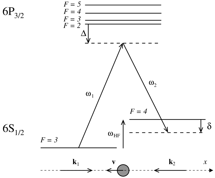
Figure 1: On top, the Raman transition for the Cesium atom. At the bottom, the beam configuration for a velocity selective transition. We have shown the usual conditions where $\delta$ and $\Delta$ are negative.

The theory of one-dimensional Raman cooling in free space, described in detail in Kasevich and Chu (1992); Moler et al. (1992), is based on a two-step cycle. We consider a cold cloud of cesium atoms initially in the hyperfine ground state $6S_{1/2},F=3$ (at this stage, we ignore the Zeeman, $m_{F}$, degeneracy). First, the atoms are placed in the light field of two off-resonant beams counter-propagating along the $x$-axis, with frequencies $\omega_{1}$ and $\omega_{2}$, and wavevectors $\mathbf{k}_{1}$ and $\mathbf{k}_{2}$ such that $\mathbf{k}_{1}\simeq-\mathbf{k}_{2}\simeq\mathbf{k}$, where $\mathbf{k}$ is a resonant wavevector for the transition $6S_{1/2}\rightarrow 6P_{3/2}$ (Fig. 1). This light field transfers the atoms with some (non zero) velocity along the beams to the other hyperfine state $6S_{1/2},F=4$, while changing their velocity by two recoil velocities $\hbar(\mathbf{k}_{1}-\mathbf{k}_{2})/M\simeq 2\hbar\mathbf{k}/M$. The detuning $\Delta$ from the $6P_{3/2}$ manifold is chosen to be much larger than the hyperfine splitting of the upper state and also large enough to avoid one-photon excitation. Second, a resonant pulse repumps the atoms to $F=3$ while giving them the possibility to reach an $x$-velocity close to zero via the emission of a spontaneous photon whose $x$-component of momentum can take any value between $\pm\hbar k$. The Raman detuning $\delta$, shown in Fig. 1 and defined as $\delta=\omega_{1}-\omega_{2}-\omega_{\mathrm{HF}}$, is chosen to select atoms with velocities $\mathbf{v}$ fulfilling the resonance condition

$$\delta=\delta_{\mathrm{LS}}+\delta_{\mathrm{D}}+4\delta_{\mathrm{rec}},$$ (1)

where

$$\delta_{\mathrm{LS}} = \frac{\Omega_{1}^{2}}{4}\left(\frac{1}{\Delta+\omega_{\mathrm{HF}}}-\frac{1}{\Delta}\right)-\frac{\Omega_{2}^{2}}{4}\left(\frac{1}{\Delta-\omega_{\mathrm{HF}}}-\frac{1}{\Delta}\right),$$

$$\delta_{\mathrm{D}} = 2\mathbf{k}\cdot\mathbf{v},$$

$$\delta_{\mathrm{rec}} = \frac{E_{\mathrm{rec}}}{\hbar}=\frac{\hbar k^{2}}{2M}.$$

In these equations, $\Omega_{1}$ and $\Omega_{2}$ are the effective electric dipole couplings of the Raman beams and $\omega_{\mathrm{HF}}$ is the hyperfine splitting. The three terms $\delta_{\mathrm{LS}}$, $\delta_{\mathrm{D}}$ and $4\delta_{\mathrm{rec}}$ are respectively the light shifts, the Raman Doppler effect and four times the recoil energy shift. This 3-level approach is a good approximation of our problem under the following conditions: the polarizations of the Raman beams are linear and the detuning $\Delta$ is large compared to the upper hyperfine splitting (see the discussion in section III.3). Choosing $\delta<0$ selects an initial velocity $\mathbf{v}$ whose $x$-component is opposed to the velocity change, which is what we want. Cooling the opposite side of the velocity distribution implies repeating the cycle with the directions of $\mathbf{k}_{1}$ and $\mathbf{k}_{2}$ reversed from that shown in Fig. 1.

Because of common mode rejection, only relative frequency noise between the Raman laser beams affects the Raman selectivity. By phase locking them relative to each other, this difference-frequency noise can be made much smaller than the noise of their separate frequencies, and negligible. The excitation spectrum is then fully determined by the shape and amplitude of the pulses. A careful tailoring of the pulse shape allows a precise excitation spectrum that does not excite atoms with a zero velocity along the $x$-axis (see for example Fig. 4a). By repeating the cooling cycle a large number of times, one forces the atoms to perform a random walk in velocity space until they hit the zero velocity state, a so-called dark state, where they tend to accumulate.

Our two-dimensional Raman cooling is a direct extension of the one-dimensional case, where the cooling cycles are alternatively applied to the $x$ and the $y$ directions.

The first Raman cooling experiments Kasevich and Chu (1992); Davidson et al. (1994) used Blackman pulses, which feature a power spectrum with very small wings outside the central peak, hence reducing off-resonant excitations. Although this might seem to be a very desirable feature, later work Reichel et al. (1995) showed experimentally and theoretically that square pulses, which produce an excitation spectrum featuring significant side lobes and a discrete set of zeros, give a better cooling in the one-dimensional case. It is also expected to be better in the two-dimensional case Reichel et al. (1995); Bardou et al. (2001). The dynamics of Raman cooling, as well as that of VSCPT, are related to non Gaussian statistics called Lévy flights Bardou et al. (2001, 1994). More precisely, for an excitation spectrum varying as $v^{\alpha}$ around $v=0$, the width of the velocity distribution scales with the cooling time $\Theta$ as $\Theta^{-1/\alpha}$. However the atoms efficiently accumulate in the cold peak of the distribution when $\Theta\rightarrow\infty$ only if $\alpha$ is greater than or equal to the dimensionality of the problem. Square pulses, for which $\alpha=2$, appear to be suitable for 2D cooling, and the present work concentrates on them.

III Experimental setup

III.1 Laser system

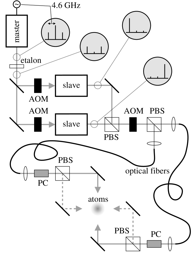
Figure 2: Schematic of the setup used to generate the Raman beams, showing the optical spectrum of the beams at various places. AOM: acousto-optic modulator; PBS: polarizing beam-splitter; PC: Pockels cell. The AOMs before the slave lasers are frequency shifters, and the AOM between the PBSs is a shutter.

Raman cooling requires two laser beams whose frequency difference is locked to a frequency close to the hyperfine frequency $\omega_{\mathrm{HF}}/2\pi\simeq 9.2\ \mathrm{GHz}$. The most common methods used to generate the two frequencies include direct electronic phase locking of two free running lasers Santarelli et al. (1994), acousto-optic modulation Bouyer et al. (1993), and electro-optic modulation Kasevich and Chu (1992). We used a different approach based on current modulation of a laser diode Ringot et al. (1999); Goldberg et al. (1983), as shown in Fig. 2. An extended-cavity master diode laser at 852$\ \mathrm{nm}$, with a free spectral range of 4.6$\ \mathrm{GHz}$, is current-modulated at $\omega_{\mathrm{HF}}/2$ in order to generate sidebands separated by $\omega_{\mathrm{HF}}$. The fraction of the power in the two first order sidebands, measured with an optical spectrum analyzer, is about 50%. The carrier is filtered out with a solid etalon having a free spectral range of 9.2$\ \mathrm{GHz}$ and a finesse of 8, and the remaining beam is used to injection-lock two slave diodes. The slave currents are adjusted in order to lock one slave to one sideband and the other slave to the other sideband. In the spectra of the slaves, the total contamination from the carrier and any of the unwanted sidebands is less than 1% of the total power. The phase coherence of the sidebands is fully transfered onto the slaves and the beatnote spectrum of the two slaves is measured  to be 1$\ \mathrm{Hz}$ wide. This includes contributions from the linewidth of the microwave generator used to modulate the master laser, the mechanical vibrations of the laser and optical system (but not of those mirrors after the fibers), and the resolution of the measurement apparatus. After transport in optical fibers, 40$\ \mathrm{mW}$ are available in each Raman beam.

As pointed out previously, cooling of opposite sides of the velocity distribution requires interchanging the directions of $\mathbf{k}_{1}$ and $\mathbf{k}_{2}$. This is done by interchanging the injection currents of the slaves so that the sidebands to which they lock are interchanged, thus interchanging their roles Szymaniec et al. (1997). The switching time, measured by monitoring the transmission of each Raman beam through a confocal cavity Szymaniec et al. (1997), is found to be about 30$\ \mathrm{\mu s}$ for a complete switch, similar to what was observed in Ref. Szymaniec et al., 1997. In the cooling experiment, we allow an extra 20$\ \mathrm{\mu s}$ as a safety margin. The swapping of the beams between the $x$ and the $y$ directions is done with Pockels cells and polarizing beam splitters (Fig. 2), in less than a microsecond. The extinction ratio of the Pockels cell switches is about 100.

III.2 Experimental details

A magneto-optical trap inside a glass cell is loaded with a few times $10^{7}$ atoms from a chirped-slowed atomic beam. The cloud has an RMS width of about 1 mm. After additional, 70$\ \mathrm{ms}$-long, molasses cooling, the atoms are dropped, pumped into $F=3$, and Raman cooled for 25$\ \mathrm{ms}$, before they fall out of the Raman beams. As shown in Fig. 3, the Raman beams are in the horizontal plane, along the $x$ and $y$ axes, providing cooling perpendicularly to the vertical direction. We found that controlling the horizontality of the Raman beams at a level of a few thousandths of a radian is enough to ensure that gravity does not perturb the cooling, but an error as large as 0.01 rad has a noticeable effect. The waist of the beams (radius at $1/e^{2}$ of peak intensity) is 4$\ \mathrm{mm}$ and they all have nominally the same power. When the atoms are dropped, they are slightly above the center of the beams, and after 25$\ \mathrm{ms}$ of cooling, they are at an approximately symmetric position below.

The repumping is provided by a retro-reflected vertical beam, tuned to the $F=4\rightarrow F^{\prime}=3$ transition, with an intensity a few times the saturation intensity and with the reflected polarization rotated in order to avoid a standing wave effect. The momentum of the photons absorbed from the repumping beams has no effect on the transverse velocity, and leads only to momentum diffusion in the vertical direction.

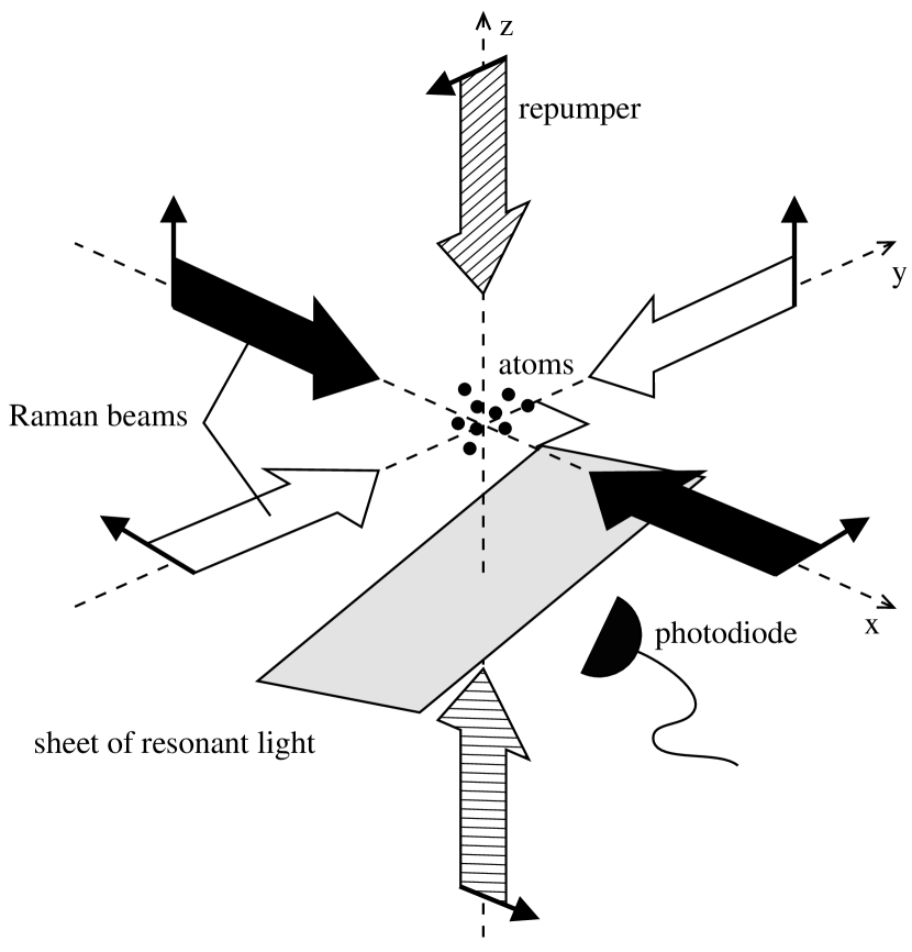
Figure 3: Geometry of the experiment. The Raman beams are in the horizontal plane, while the repumper beams are vertical. The polarizations are linear along the directions indicated by the arrows. The MOT beams are not shown. The atoms in $F=4$ are detected by fluorescence when they fall through a horizontal sheet of light resonant with the transition $F=4\rightarrow F^{\prime}=5$, located 2$\ \mathrm{cm}$ under the MOT position.

The velocity distribution along $x$ or $y$ is measured by Raman spectroscopy Kasevich et al. (1991), i.e. by transferring a narrow velocity class from $F=3$ to $F=4$ with a long Raman $\pi$ pulse. Two centimeters below the Raman beams, the atoms fall through a sheet of light tuned to the $F=4\rightarrow F^{\prime}=5$ cycling transition. The integrated fluorescence collected by a photodiode is proportional to the number of atoms transfered to the $F=4$ state. By scanning the Raman detuning $\delta$ for a succession of identically cooled atomic samples, one can probe all the velocities and reconstruct the velocity distribution. There is a small, uniform background signal; after subtraction of this background, we obtain velocity distributions such as that shown in Fig. 5.

Raman cooling as described here is essentially a 3-level scheme and our experiment requires the Zeeman sublevels to be degenerate within each hyperfine level. Good subrecoil Raman cooling can be achieved only if any Zeeman splitting is small compared to the Raman Doppler shift associated with a single recoil velocity, which is $8.2\ \mathrm{kHz}$. This is ensured by reducing the DC stray magnetic field with an opposing applied external magnetic field, and further reducing the DC and AC residual fields with a $\mu$-metal shield. Raman spectroscopy with non-velocity-selective, co-propagating beams and long pulses (300$\ \mathrm{\mu s}$) is used to optimize the field zeroing by adjusting for minimum spectral width. The Raman spectrum has a full width half maximum (FWHM) of 0.5$\ \mathrm{kHz}$, corresponding to a residual stray field smaller than $100\ \mathrm{\mu G}$, and equivalent to the Raman Doppler shift of atoms with a velocity $v_{\mathrm{rec}}/16$.

III.3 Excitation spectrum

The polarizations of each pair of Raman beams are crossed-linear in order to ensure that, because the detuning $|\Delta|$ is large compared to the hyperfine splitting (600$\ \mathrm{MHz}$) of the excited state, the light shifts are nearly the same for all the Zeeman sublevels of the ground state Miller et al. (1993). Under those conditions, the effective electrical dipole coupling $\Omega$ corresponding to an intensity $I$ has a value $\Omega=\Gamma\sqrt{0.67\;I/2I_{0}}$, where $\Gamma=2\pi\times 5.2\ \mathrm{MHz}$ is the natural linewidth of the excited state, and $I_{0}=1.1\ \mathrm{mW/cm^{2}}$ is the saturation intensity for the strongest transition. The Raman detuning $\delta$ has to be negative to cool the atoms, and is chosen in such a way that atoms with a zero velocity are resonant with the first zero point of the excitation spectrum . We extend Eq. (1) by defining the effective detuning seen by these zero velocity atoms as

$$\delta_{0}=\delta-\delta_{\mathrm{LS}}-4\delta_{\mathrm{rec}},$$

so that

$$\delta_{0}=\delta+0.67\frac{\Gamma^{2}I}{8I_{0}}\left(\frac{1}{\Delta-\omega_{\mathrm{HF}}}-\frac{1}{\Delta+\omega_{\mathrm{HF}}}\right)-\frac{2\hbar k^{2}}{M}.$$ (2)

The excitation spectrum, defined as the probability $\mathcal{P}$ of undergoing a Raman transition for any atom seeing an effective Raman detuning $\delta_{\mathrm{ex}}$, is given for a square pulse of length $t$ by the Rabi formula:

$$\mathcal{P}(\delta_{\mathrm{ex}})=\frac{\Omega_{\mathrm{R}}^{2}}{\delta_{\mathrm{ex}}^{2}+\Omega_{\mathrm{R}}^{2}}\sin^{2}\left(\frac{t}{2}\sqrt{\delta_{\mathrm{ex}}^{2}+\Omega_{\mathrm{R}}^{2}}\right),$$ (3)

where $\Omega_{\mathrm{R}}=\frac{I}{I_{0}}\cdot\frac{\Gamma^{2}}{4|\Delta|}\mathcal{C}$ is the Raman Rabi frequency. The coefficient $\mathcal{C}$ depends on the initial state in the $F=3$ manifold. It has a mean value $\overline{\mathcal{C}}=0.28$ and a total spread of $\pm 20\%$. The value of $\delta$ defined by Eq. (2) must fulfill $\mathcal{P}(\delta_{0})=0$. That is, for zero velocity atoms, $t\sqrt{\delta_{0}^{2}+\Omega_{\mathrm{R}}^{2}}=2\pi$. In the above, we have assumed that $\Omega_{1}=\Omega_{2}=\Omega$. In fact, the intensities $I_{1}$ and $I_{2}$ of the Raman beams may differ by as much as 20%. To take this into account, one would have to write Eq. (2) in the form of Eq. (1), and replace $I$ in the definition of $\Omega_{\mathrm{R}}$ with $\sqrt{I_{1}I_{2}}$.

The detuning $\delta$ depends on the light intensity in two different ways. Firstly, there is the differential light shift $\delta_{\mathrm{LS}}$ between the two hyperfine levels, which is proportional to the light intensity $I$. Secondly, according to Eq. (3), the frequency of the first zero of the excitation spectrum changes due to a “saturation” effect, as soon as $\Omega_{\mathrm{R}}t$ is not small compared to 1, that is to say when the maximum transfer probability is not small compared to unity. These dependences on the light intensity lead to complications because the Raman beams have a Gaussian profile and are never perfectly spatially homogeneous. Depending on their position in the beams, different atoms have different resonance conditions. In previous experiments Reichel et al. (1995); Reichel (1996), the differential light shift was reduced by using a detuning $\Delta$ large compare to the hyperfine splitting $\omega_{\mathrm{HF}}$, and the saturation effect was reduced by setting the maximum transfer probability to 0.5, thus using $\pi/2$ pulses instead of $\pi$ pulses.

Figure 4: Excitation spectrum of $50\ \mathrm{\mu s}$-long Raman pulses, with a maximum transfer probability of 0.8. In figures (a) and (c), the atomic cloud is centered on the Raman beams (nearly homogeneous illumination), in figures (b) and (d), the cloud is on the side of the beams (inhomogeneous illumination). The position of the dark state is indicated by the arrows. The dashed line in figure (a) is the parabola that matches the second derivative of the spectrum at the position of the dark state.

Because of a limitation in the available laser power, we worked at a detuning $|\Delta|$ of only 20$\ \mathrm{GHz}$, with pulses having a maximum transfer efficiency of 80% ($0.7\pi$-pulses). As shown below, although not negligible, the saturation shift and the light shift partially cancel out, thus limiting unwanted excitation of the dark state.

We measure the excitation spectrum by determining the transfer efficiency of such Raman pulses as a function of the Raman detuning $\delta$, with non-velocity-selective co-propagating beams. Figure 4 shows the excitation spectrum when the atomic cloud is centered on the Raman beams (a), resulting in a fairly homogeneous illumination, and when the cloud is on the edge of the beams (b), resulting in an inhomogeneous illumination. The arrows show the position of the Raman detuning corresponding to the dark state. Because the light shift and the saturation respectively shift and broaden the spectrum, locations in the cloud exposed to different light intensities yield different positions and shapes of the excitation spectrum. The spectra of the individual atoms contribute inhomogeneously to the measured spectrum. In both case (a) and (b), it appears that the spectrum is not fully symmetric and that the first minimum on the positive detuning side does not go as close to zero as does the minimum corresponding to the dark state. This comes from the fact that the saturation and the light shift have opposite effects on the position of the zero on one side of the spectrum, and similar effects on the other side. This effect becomes very visible in the inhomogeneous illumination case. However, the cancellation is not perfect, and the dispersion of the Raman coupling through the dependence of $\mathcal{C}$ on the Zeeman sublevel also leads to a “blurring” of the spectrum. As a result, the dark state features a small excitation probability, even in the homogeneous illumination case. On the time scale of our cooling sequence, this has not proven to be of importance.

With a detuning $|\Delta|=20\ \mathrm{GHz}$, our $50\ \mathrm{\mu s}$-long Raman $0.7\pi$ pulse corresponds at the center of the beam to a mean Raman Rabi frequency $\overline{\Omega}_{\mathrm{R}}=\overline{\mathcal{C}}\Gamma^{2}/4|\Delta|\cdot I/I_{0}=2\pi\times 7\ \mathrm{kHz}$, and an intensity $I\simeq 80\ \mathrm{mW/cm^{2}}$ for each beam. The probability of one-photon excitation is of the order of $\Gamma/|\Delta|$ per pulse. It results in a total probability of excitation of 10% for a typical cooling sequence of 300 pulses, which is low enough to avoid any significant perturbation of the cooling. The choice of a pulse length of 50$\ \mathrm{\mu s}$ means that the excitation spectrum covers most of the initial velocity distribution, as seen on Fig. 5.

IV Results

The elementary Raman cooling cycle is a $50\ \mathrm{\mu s}$ square Raman pulse with the $\omega_{1}$ beam along some direction, e.g. $+x$ (as in Fig. 1), and the $\omega_{2}$ beam along the opposite direction, e.g. $-x$, followed by a $10\ \mathrm{\mu s}$ resonant repumping pulse from counter-propagating beams along $z$. In this example, the elementary cycle provides cooling along the $+x$ axis. The rise and fall times of the Raman pulse are less than $1\ \mathrm{\mu s}$. In our experiment, the elementary cooling cycles are applied in pairs along a given direction. A complete cycle consists of 4 pairs of elementary cooling cycles applied successively along the directions $+x$, $+y$, $-y$ and $-x$. The full cooling sequence is typically composed of 40 complete cycles.

As pointed out previously, the switching time between perpendicular directions, limited by Pockels cell switching, is instantaneous with respect to the experimental timescale, but the switching time between parallel directions is $50\ \mathrm{\mu s}$. Using pairs of identical elementary cycles reduces the total number of complete cycles, and thus reduces the total time spent switching the beams. There is almost no loss of efficiency resulting from the application of two successive elementary cycles along the same direction because after only a few complete cooling cycles, the velocity distribution becomes narrow enough so that the atoms are in the tail of the excitation spectrum and the excitation probability per Raman pulse is small compared to 1 for most of the atoms.

Immediately after the cooling, the velocity distribution is probed with a $500\ \mathrm{\mu s}$ square $\pi$ pulse applied along the $x$ or the $y$ axis. Figure 5b shows the velocity distribution measured along the $x$ axis after 320 elementary cycles (40 complete cycles), corresponding to a $22.4\ \mathrm{ms}$ cooling sequence. The velocity spread, defined as $\sigma=\mathrm{FWHM}/\sqrt{8\ln 2}$, is reduced from about 4 $v_{\mathrm{rec}}$ after molasses cooling, corresponding to an effective temperature of 3$\ \mathrm{\mu K}$, to 0.39(5) $v_{\mathrm{rec}}$ , corresponding to an effective temperature of 30$\ \mathrm{nK}$. Note that a 20% contribution from the probe excitation linewidth is removed by deconvolution. A similar velocity distribution is measured along the $y$ axis. For either of these 1D velocity distributions, about 80% of the area is contained in the central cold peak. Most of the rest of the atoms are contained in two secondary peaks at positions where both excitation spectra are close to zero, as seen in Fig. 5a. From this we conclude  that in 2 dimensions, about 60% of the atoms are in the 2D cold peak.

It is worth noting that because we operate in the case where $\alpha$ is equal to the dimensionality of the cooling, the number of atoms in the cold peak of the 2D velocity distribution is predicted Reichel et al. (1995); Bardou et al. (2001) not to change any more as soon as we enter the subrecoil regime and the cold peak is clearly separated from the rest of the distribution. The main effect of continued cooling is to reduce the width of the cold peak without changing the number of atoms it contains. This is indeed what we observe as shown in Fig. 6.

During the entire Raman cooling process, the 2D velocity width is reduced by a factor of 10, while the size of the cloud along $x$ and $y$ does not change significantly, leading to a 100-fold increase of the 2D phase space density. Of course, taking into account the heating and expansion along the $z$ direction (which we did not measure), the increase in the 3D phase space density would be smaller, perhaps a few tens. We note however that Raman cooling in free space is not a promising way to increase the phase space density to reach quantum degeneracy because the spatial density stays roughly constant. This means that a great deal of additional cooling is required. On the other hand, a high spatial density is not desirable for clock applications, because it leads to collisional frequency shifts.

    (a)     (b)

Figure 5: (a) Velocity distribution along the $x$ axis before Raman cooling (circles), and after 15$\ \mathrm{ms}$ of 2D Raman cooling (heavy line). (b) Velocity distribution along the $x$ axis after a 22.4$\ \mathrm{ms}$ 2D Raman cooling sequence consisting of 320 Raman pulses. Also shown in both graphs in dotted and dashed lines are the excitation spectra used to cool along the directions $x$ and $-x$, tuned to match their first zeros on the dark state.

An important issue is the isotropy of the velocity distribution in the cooling plane. The cooling scheme is fundamentally anisotropic, and we only measured the velocity spread along the cooling directions $x$ and $y$. However there are good reasons to believe that the peak of cold atoms at the center of the final distribution is isotropic (in two dimensions). As indicated in Bardou et al. (1994), the dynamics of each individual atom is dominated by fairly distinct phases, where it either performs a random walk in velocity space outside the subrecoil range, or stays close to the dark state, in the subrecoil range, until it gets excited and resumes the random walk. The argument for a final isotropic velocity distribution relies on two considerations. Firstly, the total excitation probability for an atom close to the dark state during a complete cycle is isotropic. Indeed, close to the null velocity, the excitation probabilities for an elementary cycle along $\pm x$ or $\pm y$ are small compared to 1 and proportional respectively to $v_{x}^{2}$ and $v_{y}^{2}$ (power law with a coefficient $\alpha=2$), leading to a total excitation probability for the complete cycle proportional to the sum $v_{r}^{2}=v_{x}^{2}+v_{y}^{2}$. This probability only depends on the “distance” $v_{r}$ from the dark state, and is therefore isotropic. Secondly, atoms excited from the subrecoil range perform several steps during their random walk before going back to the subrecoil range at a random point which is uncorrelated with the previous position they occupied close to the dark state.

The combination of the effectively isotropic excitation of the subrecoil atoms and the homogeneous filling of the subrecoil region should produce an isotropic cold peak. We checked that a simple Monte Carlo simulation ignoring Zeeman sublevels gives a perfectly isotropic distribution in the $x-y$ plane.

We also studied the experimentally measured velocity spread $\sigma$ as a function of the cooling time $\Theta$. The results are shown on Fig. 6. As stated in section III, subrecoil cooling theory predicts that the velocity spread is described at long times by the power law $\Theta^{-1/\alpha}$, where $\alpha$ is the excitation spectrum power law coefficient. Our data do not cover a range of cooling times large enough to fully enter the asymptotic regime, and to allow an accurate experimental determination of $\alpha$. However, Fig. 6 shows that our data is compatible with cooling dynamics described by the theoretical power law $\Theta^{-1/2}$ ($\alpha=2$) at times longer than 10$\ \mathrm{ms}$.

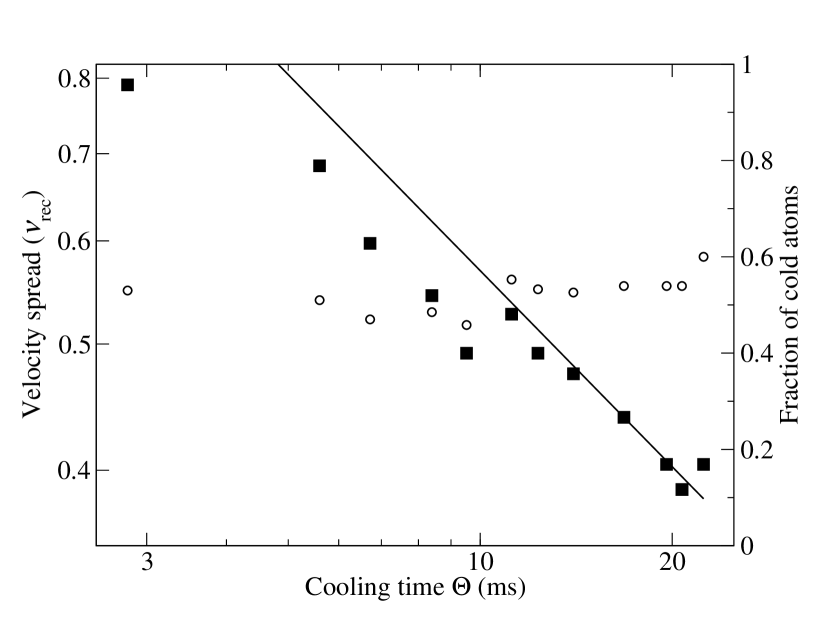
Figure 6: Filled squares: Velocity spread $\sigma$ as a function of the cooling time $\Theta$. The straight line is the power law $\beta\Theta^{-1/2}$, whose multiplicative factor $\beta$ has been adjusted manually to make the line fit the data at long times. Open circles: Fraction of atoms in the cold peak determined as explained in the text.

It is expected that because of the experimental imperfections, the velocity spread would eventually reach a finite value at long times. Nonetheless, Fig. 6 does not show any evident saturation, which indicates that a longer cooling time, for instance in micro-gravity, would lead to an even smaller velocity spread.

One of the potential limitations of Raman cooling is photon reabsorption Castin et al. (1998). However, with a spatial density less than $10^{10}\ \mathrm{cm^{-3}}$ and an optical depth of the order of unity, we do not expect photon reabsorption to hinder the cooling Perrin et al. (1999). In clock applications, the density would typically be significantly lower than in these experiments and reabsorption should be completely negligible.

To keep the cooling sequence simple, we use Raman pulses with a fixed length. The choice of 50$\ \mathrm{\mu s}$-long pulses is convenient because the resulting excitation spectrum covers most of the initial velocity distribution, and more importantly, covers the maximum excursion range of the atoms during their random walk. Indeed, an atom close to zero velocity can be pushed away from the center of the velocity distribution by a maximum amount of about 4 $v_{\mathrm{rec}}$: two recoil velocities during the Raman transition plus one or two (or exceptionally more) during the repumping process. The excitation spectrum covers 5 $v_{\mathrm{rec}}$ between the two first zeros.

It should be possible to use longer pulses (narrower excitation spectrum) in combination with short pulses (wider excitation spectrum) that recycle atoms far from zero velocity Reichel et al. (1995). The increased filtering effect of longer pulses produces an narrower distribution at the cost of a smaller number of atoms in the cold peak. In any case, the best cooling strategy results from a tradeoff between the width of the distribution and the fraction of atoms in the cold peak, and depends on the total cooling time available.

V Conclusions

Our scheme produces a narrower velocity distribution with respect to the recoil velocity than what was previously achieved with 2D Raman cooling Davidson et al. (1994). There are two main differences from that previous scheme, where the cooling was performed in a vertical plane, from the four directions at the same time. First, we use one pair of Raman beams at a time, in order to avoid unwanted excitation of the dark state. Indeed, in Ref. Davidson et al. (1994), the careful use of circular polarization avoided diffracting the atoms from standing waves created by counter-propagating beams of the same frequency, but higher order photon transitions of the type $(\omega_{1},\mathbf{k})(\omega_{2},\mathbf{-k})(\omega_{2},\mathbf{k})(\omega_{1},\mathbf{-k})$ would still be able to transfer 4 $v_{\mathrm{rec}}$ to the atoms. Second, since we cool in the horizontal plane, gravity has no effect on the velocity components which are being cooled and does not accelerate atoms out of the cold peak, allowing for a more effective cooling.

To be used in an cold-atom atomic clock, Raman cooling has to be coupled with a launching mechanism like moving molasses. An easy solution is to first launch the atoms and then collimate them with Raman cooling on their way towards the first microwave cavity. The cooling time depends on the size of the Raman beams and the launch speed.

In that perspective, our setup performs quite well in comparison with a newer scheme relying on sideband cooling in optical lattices Hamann et al. (1998), which has produced polarized samples with a velocity spread of 0.85 $v_{\mathrm{rec}}$ in 3D, in a fountain-like geometry Treutlein et al. (2001). While it is appealing for its simplicity, sideband cooling has a fundamental limit for the lowest velocity spread achievable, which is about 0.7 times the recoil velocity associated with the wavevector of the lattice used to trap the atoms Kastberg et al. (1995). Raman cooling has no such a limitation.

It is worth noticing that, although deeply subrecoil velocities are obtained for long cooling times, only accessible in micro-gravity, 2D Raman cooling can still provide subrecoil velocities in a few milliseconds, as shown in Fig. 6. Implementing the scheme on a moving-molasses earth-bound fountain, where a 1.5$\ \mathrm{cm}$-interaction region with the Raman beams combined with a typical launch velocity of 5$\ \mathrm{m/s}$ leads to an interaction time of 3$\ \mathrm{ms}$, would yield a substantial improvement in terms of brightness of the atomic source, reducing the transverse velocity spread from a few recoils to less than a recoil velocity.

For a micro-gravity-operated atomic beam, the improvement would be even more dramatic because the launch velocity can be much smaller than in a fountain, making the interaction time with the Raman beams much longer. The maximum cooling time is more likely to be limited by the maximum longitudinal heating acceptable. How the increase of brightness translates into an increase of the stability of a space-borne atomic clock depends on geometrical details and on the factors which actually limit the stability and/or the accuracy. For simplicity, let us assume that the atomic cloud is severely clipped by the opening of the second microwave cavity, as is the case in current fountain clocks, and that the signal-to-noise ratio is the main limiting factor of the short-term stability . Reducing the transverse velocity spread from 2 $v_{\mathrm{rec}}$ to 0.4 $v_{\mathrm{rec}}$ (our current result) would increase the flux of atoms through the cavity by a factor of 25. That would translate into a 5-fold increase of the signal-to-noise ratio, leading to a 5-fold increase of the short-term stability for a given averaging time, or a 25-fold reduction in the averaging time needed to achieve a given short-term stability.