Using symmetries and generating functions to calculate and minimize moments of inertia

Abstract

This paper presents some formulae to calculate moments of inertia for solids of revolution and for solids generated by contour plots. For this, the symmetry properties and the generating functions of the figures are utilized. The combined use of generating functions and symmetry properties greatly simplifies many practical calculations. In addition, the explicit use of generating functions gives the possibility of writing the moment of inertia as a functional, which in turn allows to utilize the calculus of variations to obtain a new insight about some properties of this fundamental quantity. In particular, minimization of moments of inertia under certain restrictions is possible by using variational methods.

PACS {45.40.-F, 46.05.th, 02.30.Wd}

Keywords: Moment of inertia, symmetries, center of mass, generating functions, variational methods.

1 Introduction

The moment of inertia (MI) plays a fundamental role in the mechanics of the rigid rotator [1], and is a useful tool in applied physics and engineering [2]. Hence, its explicit calculation is of greatest interest. In the literature, there are alternative methods to facilitate the calculations of MI for beginners [4], at a more advanced level [5], or using an experimental approach [6]. Most textbooks in mechanics, engineering and calculus show some methods to calculate MI’s for certain types of figures [1, 2, 3]. However, they usually do not exploit the symmetry properties of the object to make the calculation easier.

In this paper, we show some quite general formulae in which the MI’s are written in terms of generating functions. On one hand, by combining considerations of symmetry with the generating functions approach, we are able to calculate the MI’s for many solids much easier than using common techniques. On the other hand, the explicit use of generating functions permits to express the MI’s as functionals; thus, we can use the methods of the calculus of variations (CV) to study the mathematical properties of the MI for several kind of figures. In particular, minimization processes of MI’s under certain restrictions are developed by applying variational methods.

The paper is organized as follows: in Secs. 2, 3 we derive expressions for the MI’s of solids of revolution. In Sec. 4 we calculate MI’s of solids by using the contour plots of the figure, finding formulae for thin plates as a special case. Sec. 5, shows some applications of our formulae, exploring some properties of the MI by using methods of the CV. Sec. 6, contains the analysis and conclusions.

2 MI’s for solids of revolution generated around the X-axis

2.1 Moment of inertia with respect to the X-axis

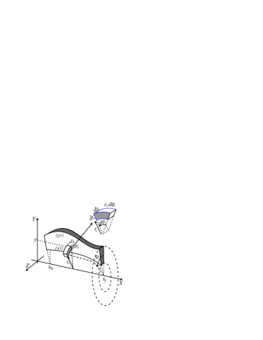
Figure 1: Solid of revolution generated from the $X-$axis. The unit of integration is a piece of hoop with cross sectional area $\left(dx\right)\left(dr_{x}\right)$ and length $r_{x}\ d\theta$. We show a rotated view of the piece of hoop in the upper right corner, for an easier visualization of its dimensions.

Let us evaluate the moment of inertia of a solid of revolution with respect to the axis that generates it, in this case the $X-$axis according to Fig. 1. We shall assume henceforth, that the solid of revolution is generated by two functions $f_{1}\left(x\right)$ and $f_{2}\left(x\right)$ that fulfill the condition $0\leq$ $f_{1}\left(x\right)\leq f_{2}\left(x\right)$ for all $x\in\left[x_{0},x_{f}\right]$.

Owing to the cylindrical symmetry exhibited by the solids of revolution, it is more convenient to work in a cylindrical system of coordinates. The coordinates are denoted by $x,r_{x},\theta$ where $r_{x}$ is the distance from the $X-$axis to the point, the coordinate $\theta$ is defined such that $\theta=0$ when the vector radius is parallel to the $Y-$axis, and increases when going from $Y$ (positive) to $Z$ (positive) as shown in Fig. 1.

We consider a thin hoop with rectangular cross sectional area equal to $\left(dx\right)\left(dr_{x}\right)$ and perimeter $2\pi r_{x}$ as Fig. 1 displays. Our infinitesimal element of volume will be a very short piece of this hoop, lying between $\theta$ and $\theta+d\theta$, the arc length for this short section of the hoop is $r_{x}\ d\theta$. Therefore, the infinitesimal element of volume and the corresponding differential of mass, are given by

$$dV=\left(dx\right)\left(dr_{x}\right)r_{x}\left(d\theta\right)\ ;\ dm=\rho\left(x,r_{x},\theta\right)\ dV\ ,$$ (2.1)

the distance from the $X-$axis  to this element of volume is $r_{x}$. Therefore, the differential moment of inertia for this element reads

$$dI_{X}=r_{x}^{2}\ dm=r_{x}^{3}\rho\left(x,r_{x},\theta\right)\left(dx\right)\left(dr_{x}\right)\left(d\theta\right)\ ,$$

and the total moment of inertia is given by

$$I_{X}=\int_{x_{0}}^{x_{f}}\left\{\int_{f_{1}\left(x\right)}^{f_{2}\left(x\right)}\left[\int_{\theta_{0}}^{\theta_{f}}\rho\left(x,r_{x},\theta\right)\ d\theta\right]r_{x}^{3}\ dr_{x}\right\}\ dx\ .$$ (2.2)

In this expression we first form the complete hoop (no necessarily closed), it means that we integrate in $\theta$ because when we form the hoop, the $x$ and $r_{x}$ variables are maintained constant and the integration only involves $\theta$ as a variable. After the completion of the hoop, we form a hollow cylinder of minimum radius $f_{1}\left(x\right)$, maximum radius $f_{2}\left(x\right)$ and height $dx$. We make it by integrating concentric hoops, where the radii $r_{x}$ of the hoops run from $f_{1}\left(x\right)$ to $f_{2}\left(x\right)$. Clearly, the variable $x$ is constant in this step of the integration. Finally, we integrate the hollow cylinders to obtain the solid of revolution, it is performed by running the $x$ variable from $x_{0}\$to$\ x_{f}$ as we can see in Fig 1. This procedure gives us the formula of Eq. (2.2).

The expression given by Eq. (2.2) is valid for any solid of revolution (characterized by the generating functions $f_{1}\left(x\right)$, $f_{2}\left(x\right)$) which can be totally inhomogeneous. Even, the revolution does not have to be from $0$ to $2\pi$. If we assume a complete revolution for the solid with $\rho=\rho\left(x,r_{x}\right)$ the formula simplifies to

$$I_{X}=2\pi\int_{x_{0}}^{x_{f}}\left[\int_{f_{1}\left(x\right)}^{f_{2}\left(x\right)}\rho\left(x,r_{x}\right)\ r_{x}^{3}\ dr_{x}\right]\ dx\ ,$$ (2.3)

and even simpler for $\rho=\rho\left(x\right)$

$$I_{X}=\frac{\pi}{2}\int_{x_{0}}^{x_{f}}\rho\left(x\right)\left[f_{2}\left(x\right)^{4}-f_{1}\left(x\right)^{4}\right]\ dx\ .$$ (2.4)

We see that all these expressions for the MI of solids of revolution along the axis of symmetry, are written in terms of the generating functions $f_{1}\left(x\right)$ and $f_{2}\left(x\right)$. In particular, it follows from Eq. (2.4) that for homogeneous solids of revolution (and even for inhomogeneous ones whose density depend only on $x$ i.e. the height of the solid), the volume integral involving the calculation of MI is reduced to a simple integral in one variable. We point out that common textbooks misuse the cylindrical properties of these type of solids, evaluating explicitly all the three integrals even for homogeneous objects.

2.2 Moments of inertia with respect to the $Y$ and $Z\$axes

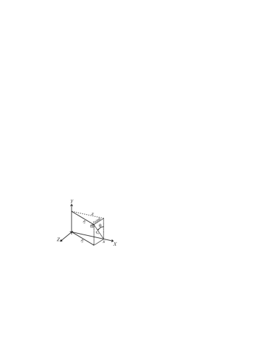
Figure 2: Distance from the $Y-$axis to a differential element of volume. In terms of the coordinates defined in Sec. 2.1 the square distance yields $r_{y}^{2}=x^{2}+r_{x}^{2}\sin^{2}\theta$.

Let us calculate the moment of inertia of the solid of revolution with respect to the $Y-$axis. We use the same element of volume of the previous section. The square distance from the $Y-$axis to such element of volume is $x^{2}+r_{x}^{2}\sin^{2}\theta$, as shown in Fig. 2. Therefore, the moment of inertia of this element of volume with respect to $Y$ reads

$$dI_{Y}=\left(r_{x}^{2}\sin^{2}\theta+x^{2}\right)\,dm\ ,$$

with $dm$ given by Eq. (2.1). Integrating in a way similar to the previous section, the MI becomes

$$I_{Y} = \int_{x_{0}}^{x_{f}}\left\{\int_{f_{1}\left(x\right)}^{f_{2}\left(x\right)}\left[\int_{\theta_{0}}^{\theta_{f}}\rho\left(x,r_{x},\theta\right)\sin^{2}\theta\ d\theta\right]r_{x}^{3}\ dr_{x}\right\}\ dx+$$ (2.5)

$$+\int_{x_{0}}^{x_{f}}\left\{\int_{f_{1}\left(x\right)}^{f_{2}\left(x\right)}\left[\int_{\theta_{0}}^{\theta_{f}}\rho\left(x,r_{x},\theta\right)\ d\theta\right]r_{x}\ dr_{x}\right\}x^{2}\ dx\ .$$

Once again, this formula is valid for any inhomogeneous solid of revolution (even incomplete) generated by the functions $f_{1}\left(x\right)$, $f_{2}\left(x\right)$. When assuming a complete solid of revolution with $\rho=\rho\left(x,r_{x}\right)$, and taking into account Eq. (2.3), the latter formula reduces to

$$I_{Y}=\frac{1}{2}I_{X}+2\pi\int_{x_{0}}^{x_{f}}x^{2}\left[\int_{f_{1}\left(x\right)}^{f_{2}\left(x\right)}\rho\left(x,r_{x}\right)\ r_{x}\ dr_{x}\right]\ dx\ .$$ (2.6)

From this expression we derive the interesting property $I_{Y}\geq I_{X}/2$, which is valid for any complete solid of revolution with azimuthal symmetry. Additionally, for $\rho=\rho\left(x\right)$ we have

$$I_{Y}=\frac{1}{2}I_{X}+\pi\int_{x_{0}}^{x_{f}}\rho\left(x\right)\ x^{2}\left[f_{2}\left(x\right)^{2}-f_{1}\left(x\right)^{2}\right]\ dx\ .$$ (2.7)

By the same token, for the $Z-$axis, which is perpendicular to the $X$ and $Y-$axes and with the origin as the intersection point, we have the following general formula

$$I_{Z} = \int_{x_{0}}^{x_{f}}\left\{\int_{f_{1}\left(x\right)}^{f_{2}\left(x\right)}\left[\int_{\theta_{0}}^{\theta_{f}}\rho\left(x,r_{x},\theta\right)\cos^{2}\theta\ d\theta\right]r_{x}^{3}\ dr_{x}\right\}\ dx+$$ (2.8)

$$+\int_{x_{0}}^{x_{f}}\left\{\int_{f_{1}\left(x\right)}^{f_{2}\left(x\right)}\left[\int_{\theta_{0}}^{\theta_{f}}\rho\left(x,r_{x},\theta\right)\ d\theta\right]r_{x}\ dr_{x}\right\}x^{2}\ dx\ .$$

We emphasize that in the case of a complete revolution, the formula (2.8), coincides exactly with $I_{Y}$ in Eq. (2.6) when $\rho$ does not depend on $\theta$, as expected from the cylindrical symmetry. Indeed, for $I_{Z}$ to be equal to $I_{Y}$, the requirement of azimuthal symmetry could be softened by demanding the conditions

$$\rho=\rho\left(x,r_{x}\right)\rho\left(\theta\right)\ \ ;\ \ \int_{\theta_{0}}^{\theta_{f}}\rho\left(\theta\right)\sin^{2}\theta\ d\theta=\int_{\theta_{0}}^{\theta_{f}}\rho\left(\theta\right)\cos^{2}\theta\ d\theta\ ,$$ (2.9)

for if the conditions (2.9) are held, we get that

$$\int_{\theta_{0}}^{\theta_{f}}\rho\left(\theta\right)\cos^{2}\theta\ d\theta=\frac{1}{2}\int_{\theta_{0}}^{\theta_{f}}\rho\left(\theta\right)\ d\theta\ ,$$

and $I_{Y}=I_{Z}$ even for an incomplete solid of revolution with no azimuthal symmetry.

From Eqs. (2.5-2.8), we see that for the calculation of the MI for axes perpendicular to the axis of symmetry, we use the same limits of integration as for the symmetry axis; thus, we do not have to care about the partitions. Once again, these MI’s are written in terms of the generating functions of the solid $f_{1}\left(x\right)$ and $f_{2}\left(x\right)$.

Finally, we emphasize that textbooks do not usually report the moments of inertia for solids of revolution with respect to axes perpendicular to the axis of symmetry. However, they are important in many physical problems. For instance, a solid of revolution acting as a physical pendulum requires the calculation of such MI’s, see example 8.

Figure 3: Frustum of a right circular cone with a conical well as a solid of revolution. The shadowed surface is the one that generates the solid. $f_{1}\left(x\right)$ and $f_{2}\left(x\right)$ are the functions that provide the limits of integration.

Example 1

MI’s for a truncated cone with a conical well (see Fig. 3). The generating functions read

$$f_{1}\left(x\right) = \left\{\begin{array}[]{ccc}R\left(1-\frac{x}{h}\right)&if&x\in\left[0,h\right]\\[2.84526pt] 0&if&x\in\left(h,H\right]\end{array}\right.$$ (2.12)

$$f_{2}\left(x\right) = \left(\frac{a_{1}-a_{2}}{H}\right)x+a_{2}\ ,$$ (2.13)

where all the dimensions involved are displayed in Fig. 3. For uniform density, we can replace Eqs. (2.13) into Eqs. (2.4, 2.7) to get

$$I_{X} = \frac{\pi\rho}{10}\left\{H\left(a_{1}^{4}+a_{2}^{4}+a_{1}a_{2}^{3}+a_{1}^{3}a_{2}+\allowbreak a_{1}^{2}a_{2}^{2}\right)-R^{4}h\right\}$$

$$I_{Y} = I_{Z}=\frac{1}{2}I_{X}+\frac{\pi\rho H^{3}}{5}\left[\frac{1}{2}a_{1}a_{2}+a_{1}^{2}+\frac{1}{6}a_{2}^{2}-\frac{R^{2}}{6}\left(\frac{h}{H}\right)^{3}\right]\ .$$

It is more usual to give the radius of gyration (RG) instead of the MI. For this we calculate the mass of the solid by using Eq. (A.1), finding

$$M=\frac{\pi\rho}{3}\left[\allowbreak H\left(a_{1}a_{2}+a_{1}^{2}+a_{2}^{2}\right)-\allowbreak R^{2}h\right]\ .$$ (2.14)

The radii of gyration become

$$K_{X}^{2} = \frac{3\left\{\allowbreak H\left(a_{1}^{4}+a_{2}^{4}+a_{1}a_{2}^{3}+a_{1}^{3}a_{2}+\allowbreak a_{1}^{2}a_{2}^{2}\right)-R^{4}h\right\}}{10\left[\allowbreak H\left(a_{1}a_{2}+a_{1}^{2}+a_{2}^{2}\right)-\allowbreak R^{2}h\right]}$$

$$K_{Y}^{2} = K_{Z}^{2}=\frac{K_{X}^{2}}{2}+\frac{3}{5}H^{3}\frac{\left[\frac{1}{2}a_{1}a_{2}+a_{1}^{2}+\frac{1}{6}a_{2}^{2}-\frac{R^{2}}{6}\left(\frac{h}{H}\right)^{3}\right]}{\left[\allowbreak H\left(a_{1}a_{2}+a_{1}^{2}+a_{2}^{2}\right)-\allowbreak R^{2}h\right]}\ .$$ (2.15)

By making $R=0$ (and/or $h=0$) we find the RG’s for the truncated cone. With $R=0$ and $a_{1}=0$, we get the RG’s of a cone for which the axes $Y$ and $Z$ pass through its base. Making $R=0$ and $a_{2}=0$, we find the RG’s of a cone but with the axes $Y$ and $Z$ passing through its vertex. Finally, by setting up $R=0$, and $a_{1}=a_{2}$; we obtain the RG’s for a cylinder. In many cases of interest, we need to calculate the MI’s for axes $X_{C}Y_{C}Z_{C}$ passing through the center of mass (CM), these MI’s can be calculated by finding the position of the CM with respect to the original coordinate axes, and using Steiner’s theorem (also known as “the parallel axis theorem”). Applying Eqs. (A.2-A.4) the position of the CM for the truncated cone with a conical well is given by $\left(x_{CM},0,0\right)$ with

$$x_{CM}=\frac{\left[\left(2a_{1}a_{2}+3a_{1}^{2}+a_{2}^{2}\right)H^{2}-R^{2}h^{2}\right]}{4\left[\allowbreak H\left(a_{1}a_{2}+a_{1}^{2}+a_{2}^{2}\right)-\allowbreak R^{2}h\right]}\ .$$ (2.16)

Gathering Eqs. (2.15, 2.16) we find

$$K_{X_{C}}^{2}=K_{X}^{2}\ ;\ K_{Y_{C}}^{2}=K_{Y}^{2}-x_{CM}^{2}\ ;\ K_{Z_{C}}^{2}=K_{Z}^{2}-x_{CM}^{2}\ .$$

2.3 Another alternative of calculation and a proof of consistency

In addition to the the parallel and the perpendicular axis theorems, there is another useful theorem about MI’s that is not usually included in common texts, namely [7]

$$I_{X}+I_{Y}+I_{Z}=2\sum\limits_{i}m_{i}R_{i}^{2}\ ,$$ (2.17)

where $X,Y,Z$ are three mutually perpendicular intersecting axes,$\ m_{i}$ is the mass of the $i-$th particle and $R_{i}$ is its distance from the intersection. We shall see that our general formulae for MI’s of solids of revolution, fulfill the theorem. From Eqs. (2.2, 2.5, 2.8) we have

$$I_{X}+I_{Y}+I_{Z}=2\int_{x_{0}}^{x_{f}}\int_{f_{1}\left(x\right)}^{f_{2}\left(x\right)}\int_{\theta_{0}}^{\theta_{f}}\left(x^{2}+r_{x}^{2}\right)\rho\left(x,r_{x},\theta\right)\ r_{x}\ \left(d\theta\right)\left(dr_{x}\right)\left(dx\right)\ .$$ (2.18)

Moreover, if we take into account that the distance from the intersecting point (the origin of coordinates) to the element of volume is $R^{2}=x^{2}+r_{x}^{2}$, and using Eq. (2.1) we conclude that

$$I_{X}+I_{Y}+I_{Z}=2\int_{V}R^{2}\ dm\ ,$$ (2.19)

which is the continuous version of the theorem established in Eq. (2.17). As well as providing a proof of consistency, this theorem could reduce the task to estimate the MI’s, especially when a certain spherical symmetry is involved.

Further, it is interesting to see that the MI’s $I_{X},I_{Y},I_{Z},$ in Eqs. (2.2, 2.5, 2.8) fulfill the triangular inequalities

$$I_{X}\leq I_{Y}+I_{Z}\ ,$$

and same for any cyclic change of the labels. The triangular inequalities follow directly from the definition of MI, and are valid for any arbitrary object. Though the demostration of these inequalities is straightforward, they are not usually considered in the literature. In the case of thin plates, one of them becomes an equality.

Example 2

The following example shows the usefulness of the theorem of Eqs. (2.17, 2.19) in practical calculations. Let us consider the MI of a sphere centered at the origin, whose density is factorizable in spherical coordinates such that $\rho=\rho(R)$. Where $R$ is the distance from the origin of coordinates to the point. The symmetry of $\rho$ leads to $I_{X}=I_{Y}=I_{Z}$ and the theorem in Eq. (2.19) gives

$$3I_{X}=8\pi\int_{0}^{R_{0}}\rho\left(R\right)\ R^{4}\ dR\ ,$$ (2.20)

the mass of the sphere is

$$M=4\pi\int_{0}^{b}\rho(R)R^{2}\ dR\ ,$$ (2.21)

from which the moment of inertia can be written as

$$I_{X}=\frac{2}{3}M\frac{\int_{0}^{b}\rho(R)R^{4}\ dR}{\int_{0}^{b}\rho(R)R^{2}\ dR}\ .$$ (2.22)

We can calculate for instance, the classical MI of an electron in a hydrogen-like atom, with respect to an axis that passes through its CM. For example, for the state $\left(1,0,0\right)$ we have that $\rho(R)=2\left(Z/a_{0}\right)^{3/2}e^{-ZR/a_{0}}$, where $Z$ is the atomic number and $a_{0}$ the Bohr’s radius. The MI becomes

$$I_{X}=\frac{8m_{e}}{Z^{2}}a_{0}^{2}\ .$$

3 MI’s of solids of revolution generated around the Y-axis

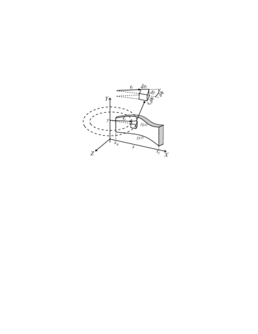
Figure 4: Solid of revolution generated around the $Y-$axis. The unit of integration is a piece of hoop with cross sectional area $\left(dy\right)\left(dr_{y}\right)$ and length $r_{y}\ d\phi$.

By using a couple of generating functions $f_{1}\left(x\right)$ and $f_{2}\left(x\right)\$like in the previous section, we are able to generate another solid of revolution by rotating such functions around the $Y-$axis instead of the $X-$axis as Fig. 4 displays. In this case however, we should assume that $x_{0}\geq 0$; such that all points in the generating surface have always non-negative $x$ coordinates. Instead, we might allow the functions $f_{1}\left(x\right)$, $f_{2}\left(x\right)$ to be negative though still demanding that $f_{1}\left(x\right)\leq f_{2}\left(x\right)$ in the whole interval of $x$. In this case, it is more convenient to use another cylindrical system in which we define the coordinates $\left(r_{y},y,\phi\right)$, where $r_{y}$ is the distance from the $Y-$axis to the point, and the angle $\phi$ has been defined such that $\phi=0$ when the vector radius is parallel to the $Z-$axis (positive), increasing when going from $Z$ (positive) to $X$ (positive). One important comment is in order, since the surface that generates the solid lies on the $XY-$plane, the $x$ coordinate of any point of this surface (which is always non-negative according to our assumptions) coincides with the coordinate$\ r_{y}$, therefore we shall write $f_{1}\left(r_{y}\right)\$and $f_{2}\left(r_{y}\right)$ instead of $f_{1}\left(x\right),\ f_{2}\left(x\right)$ for the functions that bound the generating surface.

The procedure to evaluate the MI in the general case is analogous to the techniques used in section 2, the results are

$$I_{X} = \int_{x_{0}}^{x_{f}}\left\{\int_{f_{1}\left(r_{y}\right)}^{f_{2}\left(r_{y}\right)}\left[\int_{\phi_{0}}^{\phi_{f}}\rho\left(r_{y},y,\phi\right)\cos^{2}\phi\ d\phi\right]\ dy\right\}r_{y}^{3}\ dr_{y}+$$ (3.1)

$$+\int_{x_{0}}^{x_{f}}\left\{\int_{f_{1}\left(r_{y}\right)}^{f_{2}\left(r_{y}\right)}\left[\int_{\phi_{0}}^{\phi_{f}}\rho\left(r_{y},y,\phi\right)d\phi\right]\ y^{2}\ dy\right\}r_{y}\ dr_{y}\ ,$$

$$I_{Y}=\int_{x_{0}}^{x_{f}}\left\{\int_{f_{1}\left(r_{y}\right)}^{f_{2}\left(r_{y}\right)}\left[\int_{\phi_{0}}^{\phi_{f}}\rho\left(r_{y},y,\phi\right)d\phi\right]\ dy\right\}r_{y}^{3}\ dr_{y}\ ,$$ (3.2)

$$I_{Z} = \int_{x_{0}}^{x_{f}}\left\{\int_{f_{1}\left(r_{y}\right)}^{f_{2}\left(r_{y}\right)}\left[\int_{\phi_{0}}^{\phi_{f}}\rho\left(r_{y},y,\phi\right)\sin^{2}\phi\,d\phi\right]\ dy\right\}r_{y}^{3}\ dr_{y}+$$ (3.3)

$$+\int_{x_{0}}^{x_{f}}\left\{\int_{f_{1}\left(r_{y}\right)}^{f_{2}\left(r_{y}\right)}\left[\int_{\phi_{0}}^{\phi_{f}}\rho\left(r_{y},y,\phi\right)d\phi\right]\ y^{2}\ dy\right\}r_{y}\ dr_{y}\ .$$

As before, these expressions become simpler in the case of a complete revolution with azimuthal symmetry,

$$I_{Y}=2\pi\int_{x_{0}}^{x_{f}}\left[\int_{f_{1}\left(r_{y}\right)}^{f_{2}\left(r_{y}\right)}\rho\left(r_{y},y\right)\ dy\right]\ r_{y}^{3}\ dr_{y}\ ,$$ (3.4)

$$I_{X}=\frac{1}{2}I_{Y}+2\pi\int_{x_{0}}^{x_{f}}\left[\int_{f_{1}\left(r_{y}\right)}^{f_{2}\left(r_{y}\right)}\rho\left(r_{y},y\right)\ y^{2}\ dy\right]r_{y}\ dr_{y}\ ,$$ (3.5)

and in this case $I_{X}=I_{Z}$, as expected from symmetry arguments. Further, assuming $\rho=\rho\left(r_{y}\right)$ the expressions simplifies to

$$I_{Y}=2\pi\int_{x_{0}}^{x_{f}}r_{y}^{3}\ \rho\left(r_{y}\right)\left[f_{2}\left(r_{y}\right)-f_{1}\left(r_{y}\right)\right]\ dr_{y}\ ,$$ (3.6)

$$I_{X}=I_{Z}=\frac{1}{2}I_{Y}+\frac{2\pi}{3}\int_{x_{0}}^{x_{f}}\rho\left(r_{y}\right)\left[\ f_{2}\left(r_{y}\right)^{3}-f_{1}\left(r_{y}\right)^{3}\right]r_{y}\ dr_{y}\ .$$ (3.7)

We can verify again that the property $I_{X}=I_{Z}\geq I_{Y}/2$ appears in the case of azimuthal symmetry, Eq. (3.5). This property is also satisfied in the case of incomplete solids of revolution, if conditions analogous to Eq. (2.9) for the $\phi$ angle are fulfilled. Moreover, the theorem given by Eqs. (2.17, 2.19) is also held by these formulae, giving an alternative way for the calculation. Finally, the triangular inequalities also hold.

These formulae are especially useful in the case in which the generating functions $f_{1}\left(x\right)$,$\ f_{2}\left(x\right)\$do not admit inverses, since in such case we cannot find the corresponding inverse functions $g_{1}\left(x\right)$,$\ g_{2}\left(x\right)$ to generate the same figure by rotating around the $X-$axis. This is the case in the following example

Figure 5: Solid of revolution created by rotating the generating functions $f_{1}\left(x\right)=0$, and $f_{2}\left(x\right)=h+A\sin\left(\frac{n\pi x}{R}\right)$ around the $Y-$axis. The $x\$variable lies in the interval $\left[0,R\right]$. From the picture it is clear that one of the generators do not admit an inverse.

Example 3

Calculate the MI’s of a homogeneous solid formed by rotating the functions

$$f_{1}\left(x\right)=0\ ;\ f_{2}\left(x\right)=h+A\sin\left(\frac{n\pi x}{R}\right)\ ,$$ (3.8)

around the $Y-axis\$(see Fig. 5), where the functions are defined in the interval $x\in\left[0,R\right]$, and $n$ are positive integers. We demand $h\geq\left|A\right|$, if $n>1$; besides, if $n=1$ and $\left|A\right|>h$ we demand $A>0$. These requirements assure that $f_{2}\left(x\right)\geq f_{1}\left(x\right)$ for all $x\in\left[0,R\right]$. The mass of the solid, obtained from (A.8) reads

$$M=\frac{\pi R^{2}\rho}{n\pi}\left[n\pi h+2A\left(-1\right)^{n+1}\right]$$

and replacing the generating functions into the Eqs. (3.6, 3.7) we get

$$K_{Y}^{2} = \frac{R^{2}}{2}\left(\frac{n\pi h+4A(6n^{-2}\pi^{-2}-1)(-1)^{n}}{n\pi h+2A(-1)^{n+1}}\right)$$

$$K_{X}^{2} = K_{Z}^{2}=\frac{K_{Y}^{2}}{2}+\frac{1}{18}\frac{3n\pi h[2h^{2}+3A^{2}]+4A(-1)^{n+1}[9h^{2}+2A^{2}]}{[n\pi h+2A(-1)^{n+1}]}\ .$$

the position of the CM (obtained from Eqs. A.5-A.7), and the RG’s for axes that pass through the CM read

$$\mathbf{r}_{CM} = \left(0,y_{CM},0\right)\ \ ;\ \ y_{CM}=\frac{2n\pi h^{2}+n\pi A^{2}+8Ah\left(-1\right)^{n+1}}{4\left[n\pi h+2A\left(-1\right)^{n+1}\right]}$$

$$K_{X_{C}}^{2} = K_{X}^{2}-y_{CM}^{2}\ ;\ K_{Y_{C}}^{2}=K_{Y}^{2}\ ;\ K_{Z_{C}}^{2}=K_{Z}^{2}-y_{CM}^{2}$$

Observe that $f_{2}\left(x\right)$ does not have inverse. Hence, we cannot generate the same figure by constructing an equivalent function to be rotated around the $X-$axis.

Finally, it worths pointing out that by considering homogeneous solids of revolution, we obtain the same expressions derived with a different approach in Ref. [8].

4 Moments of inertia based on the contour plots of some figures

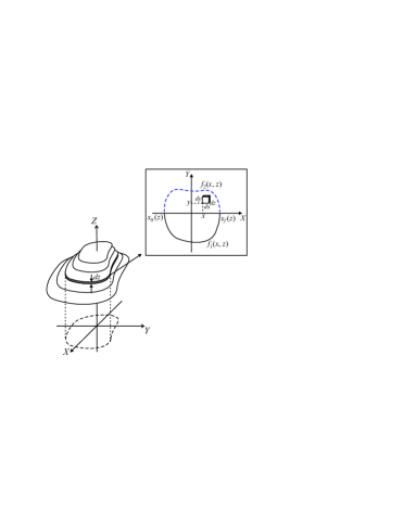
Figure 6: Contour plots of a solid utilized to calculate its moments of inertia.

Suppose that we know the contour plots of certain solid in the $XY$ plane, i.e. the surfaces shaped by the intersection between planes parallel to the $XY$ plane and the solid (see Fig. 6). Assume that for a certain value of the $z$ coordinate, the surface defined by the contour is bounded by the functions $f_{1}\left(x,z\right)$ and $f_{2}\left(x,z\right)$ in the $y$ coordinate, and by $x_{0}\left(z\right)$, $x_{f}\left(z\right)$ in the $x$ coordinate, as shown in the frame on the upper right corner of Fig. 6. Let us form a thin plate of thick $dz$ with the surface described above. In turn we can divide such thin plate into small rectangular boxes with surface $dx\ dy$ and depth $dz$ as shown in Fig. 6, it is well known from the literature [1] that the MI with respect to the $X-$axis in cartesian coordinates reads

$$I_{X}=\int_{V}\left(y^{2}+z^{2}\right)\ dm$$

now, since our infinitesimal elements of volume are rectangular boxes with volume $dV=dx\ dy\ dz$, the contribution of each rectangular box to the MI around the $X-$axis is given by

$$dI_{X}=\left(y^{2}+z^{2}\right)\ dm=\left(y^{2}+z^{2}\right)\rho\left(x,y,z\right)\ dx\ dy\ dz\ ,$$

integrating over all variables, we obtain

$$I_{X}=\int_{z_{0}}^{z_{f}}\left\{\int_{x_{0}\left(z\right)}^{x_{f}\left(z\right)}\left[\int_{f_{1}\left(x,z\right)}^{f_{2}\left(x,z\right)}y^{2}\rho\ dy\right]dx\right\}dz+\int_{z_{0}}^{z_{f}}\left\{\int_{x_{0}\left(z\right)}^{x_{f}\left(z\right)}\left[\int_{f_{1}\left(x,z\right)}^{f_{2}\left(x,z\right)}\rho\ dy\right]dx\right\}z^{2}\ dz\ .$$ (4.1)

The procedure for $I_{Y}$ and $I_{Z}$ is analogous, the results are.

$$I_{Y} = \int_{z_{0}}^{z_{f}}\left\{\int_{x_{0}\left(z\right)}^{x_{f}\left(z\right)}\left[\int_{f_{1}\left(x,z\right)}^{f_{2}\left(x,z\right)}\rho\ dy\right]x^{2}\ dx\right\}dz+\int_{z_{0}}^{z_{f}}\left\{\int_{x_{0}\left(z\right)}^{x_{f}\left(z\right)}\left[\int_{f_{1}\left(x,z\right)}^{f_{2}\left(x,z\right)}\rho\ dy\right]dx\right\}z^{2}\ dz\ ,$$ (4.2)

$$I_{Z} = \int_{z_{0}}^{z_{f}}\left\{\int_{x_{0}\left(z\right)}^{x_{f}\left(z\right)}\left[\int_{f_{1}\left(x,z\right)}^{f_{2}\left(x,z\right)}y^{2}\rho\ dy\right]dx\right\}dz+\int_{z_{0}}^{z_{f}}\left\{\int_{x_{0}\left(z\right)}^{x_{f}\left(z\right)}\left[\int_{f_{1}\left(x,z\right)}^{f_{2}\left(x,z\right)}\rho\ dy\right]x^{2}\ dx\right\}dz\ .$$ (4.3)

Once again, we can check that results (4.1, 4.2, 4.3) satisfy Eq. (2.19). This equation gives us another way to calculate the three MI’s. Finally, the formulae fulfill the triangular inequalities.

An interesting case arises when we consider the MI’s of thin plates. Suppose a thin plate lying on the XY plane. $\sigma\left(x,y\right)$ denotes its surface density. This solid is generated by contour plots with volumetric density

$$\rho\left(x,y,z\right)=\sigma\left(x,y\right)\ \delta\left(z\right)\ ,$$ (4.4)

where $\delta\left(z\right)$ denotes Dirac’s delta function. Replacing Eq. (4.4) into the general formula (4.1) we get

$$I_{X} = \int_{z_{0}}^{z_{f}}H_{1}\left(z\right)\ \delta\left(z\right)\ dz+\int_{z_{0}}^{z_{f}}H_{2}\left(z\right)\ \delta\left(z\right)\ z^{2}\ dz\ ,$$

$$H_{1}\left(z\right) \equiv \int_{x_{0}\left(z\right)}^{x_{f}\left(z\right)}\left[\int_{f_{1}\left(x,z\right)}^{f_{2}\left(x,z\right)}y^{2}\sigma\left(x,y\right)\ dy\right]dx\ ;\ H_{2}\left(z\right)\equiv\int_{x_{0}\left(z\right)}^{x_{f}\left(z\right)}\left[\int_{f_{1}\left(x,z\right)}^{f_{2}\left(x,z\right)}\sigma\left(x,y\right)\ dy\right]dx\ ,$$

and using the properties of $\delta\left(z\right)$ we get

$$I_{X}=H_{1}\left(0\right)=\int_{x_{0}\left(0\right)}^{x_{f}\left(0\right)}\left[\int_{f_{1}\left(x,0\right)}^{f_{2}\left(x,0\right)}y^{2}\sigma\left(x,y\right)\ dy\right]dx\ ,$$

the $z$ coordinate is evaluated at zero all the time, hence there is only one contour, we write it simply as

$$I_{X}=\int_{x_{0}}^{x_{f}}\left[\int_{f_{1}\left(x\right)}^{f_{2}\left(x\right)}y^{2}\sigma\left(x,y\right)\ dy\right]dx\ .$$ (4.5)

Similarly $I_{Y},\ I_{Z}$ can be evaluated replacing (4.4) into (4.2) and (4.3)

$$I_{Y}=\int_{x_{0}}^{x_{f}}\left[\int_{f_{1}\left(x\right)}^{f_{2}\left(x\right)}\sigma\left(x,y\right)\ dy\right]x^{2}\ dx\ ;\ I_{Z}=I_{X}+I_{Y}\ .$$ (4.6)

Hence, Eqs. (4.5, 4.6) give us the MI’s for a thin plate delimited by $f_{1}\left(x\right)$ and $f_{2}\left(x\right)$ and by $x_{0}$,$\ x_{f}$; with surface density $\sigma\left(x,y\right)$. It worths noting that the second of Eqs. (4.6) arises from the application of (4.4) into (4.3) without assuming the perpendicular axes theorem; showing the consistency of our results.

The formulae shown in this section are written in terms of generating functions as in the previous sections. However, these generators are functions of several variables. In developing these formulae we have not used any particular symmetry; nevertheless, explicit use of some symmetries could simplify many specific calculations as shown in the following examples.

Figure 7: Frustum of a right elliptical cone. The shadowed surfaces show a contour for a certain value of the $z$ coordinate, as well as its projection onto the $XY-$plane.

Example 4

Let us assume a truncated right elliptical cone as shown in Fig. 7. Such figure is characterized by the semi-major and semi-minor axes in the base (denoted by $a_{1}$,$b_{1}$ respectively), its height $H$, and its semi-major and semi-minor axes in the top (denoted by$\ a_{2}$, $b_{2}$ respectively). Suppose that the truncated cone is located such that the major base lies on the $XY$ plane and the center of such major base is on the origin of coordinates, as shown in Fig. 7. Now, since we are assuming that the figure is not oblique, then all the contours (see right top on Fig. 7) are concentric ellipses centered at the origin, with the same eccentricity. Therefore, it is more convenient to describe such ellipses in terms of their eccentricity $\varepsilon\$and the semi-major axis $a\left(z\right)$. The contours are then delimited by

$$f_{1}\left(x,z\right) = -\sqrt{\left[a\left(z\right)^{2}-x^{2}\right]\left(1-\varepsilon^{2}\right)}\ ;\ f_{2}\left(x,z\right)=\sqrt{\left[a\left(z\right)^{2}-x^{2}\right]\left(1-\varepsilon^{2}\right)}\ ,$$

$$x_{0}\left(z\right) = -a\left(z\right)\ ;\ x_{f}\left(z\right)=a\left(z\right)\ ;\ \varepsilon\equiv\sqrt{1-\left(\frac{b\left(z\right)}{a\left(z\right)}\right)^{2}}\ ,$$ (4.7)

where $f_{1,2}\left(x,z\right)$ are the functions that generate the complete ellipse of semi-major axis $a\left(z\right)$ and eccentricity $\varepsilon\$(independent of $z$). By simple geometric arguments, we could see that the semi-major axis of one contour of the truncated cone at certain height $z$ is given by

$$a\left(z\right)=a_{1}+\left(\frac{a_{2}-a_{1}}{H}\right)z\ ,$$ (4.8)

Assuming that the density is constant Eq. (4.3) becomes

$$I_{Z} = \frac{2\rho}{3}\left(\sqrt{1-\varepsilon^{2}}\right)^{3}\int_{0}^{H}\left\{\int_{-a\left(z\right)}^{a\left(z\right)}\left[\left(\sqrt{a\left(z\right)^{2}-x^{2}}\right)^{3}\right]dx\right\}dz$$

$$+2\rho\sqrt{1-\varepsilon^{2}}\int_{0}^{H}\left\{\int_{-a\left(z\right)}^{a\left(z\right)}\left[\sqrt{a\left(z\right)^{2}-x^{2}}\right]x^{2}\ dx\right\}dz\ ,$$

where we have already made the integration in $y$. Integration in $x$ yields

$$I_{Z}=\frac{\pi\rho}{4}\left(2-\varepsilon^{2}\right)\sqrt{1-\varepsilon^{2}}\left[\int_{0}^{H}a\left(z\right)^{4}\ dz\right]\ ,$$ (4.9)

and taking into account the Eq. (4.8) we find

$$I_{Z}=\frac{\pi\rho H}{20}\left(2-\varepsilon^{2}\right)\sqrt{1-\varepsilon^{2}}\left[a_{1}^{4}+a_{2}^{4}+a_{1}a_{2}^{3}+a_{1}^{3}a_{2}+a_{1}^{2}a_{2}^{2}\right]\ .$$ (4.10)

Now, the mass of the figure is obtained from Eq. (A.12) and reads

$$M=\frac{\pi\rho H}{3}\sqrt{1-\varepsilon^{2}}\left(a_{1}^{2}+a_{2}^{2}+a_{1}a_{2}\right)\ ,$$ (4.11)

therefore, the radius of gyration $K_{Z}^{2}\$could be written as

$$K_{Z}^{2}=\frac{3}{20}\left(2-\varepsilon^{2}\right)\left[\frac{a_{1}^{4}+a_{2}^{4}+a_{1}a_{2}^{3}+a_{1}^{3}a_{2}+a_{1}^{2}a_{2}^{2}}{a_{1}a_{2}+a_{1}^{2}+a_{2}^{2}}\right]\ .$$

Further, $K_{X}^{2}$ and $K_{Y}^{2}$ can be derived from Eqs. (4.1, 4.2, 4.11) obtaining

$$K_{X}^{2} = \frac{3}{20}\frac{\left[\left(1-\varepsilon^{2}\right)\left(a_{1}^{4}+a_{2}^{4}+a_{1}a_{2}^{3}+a_{1}^{3}a_{2}+\allowbreak a_{1}^{2}a_{2}^{2}\right)+4H^{2}\left(a_{2}^{2}+\frac{1}{6}a_{1}^{2}+\frac{1}{2}a_{1}a_{2}\right)\right]}{\left(a_{1}^{2}+a_{2}^{2}+a_{1}a_{2}\right)}$$

$$K_{Y}^{2} = \frac{3}{20}\frac{\left[\left(a_{1}^{4}+a_{2}^{4}+a_{1}a_{2}^{3}+a_{1}^{3}a_{2}+\allowbreak a_{1}^{2}a_{2}^{2}\right)+4H^{2}\left(a_{2}^{2}+\frac{1}{6}a_{1}^{2}+\frac{1}{2}a_{1}a_{2}\right)\right]}{\left(a_{1}^{2}+a_{2}^{2}+a_{1}a_{2}\right)}\ .$$

when $\varepsilon=0$ we get the radii of gyration of a truncated cone with circular cross section. In addition, when $\varepsilon=0$ and $a_{2}=0$, the RG’s reduce to the expressions for a cone with the axes $X$ and $Y$ passing through its base. Setting $\varepsilon=0,$ $a_{1}=0$, we also get the RG’s of a cone but with the $X,Y$ axes passing through its vertex. Using $\varepsilon=0,$ $a_{1}=a_{2}$ we obtain the RG’s of a cylinder. Finally, with $a_{2}=0$ we get a cone with elliptical cross section, and when $a_{1}=a_{2}$ we obtain a cylinder with elliptical cross section. Now, if we are interested in the MI for coordinates ($X_{C},Y_{C},Z_{C}$) passing through the CM, we should calculate the position of the CM from Eqs. (A.9-A.11) and use Steiner’s theorem obtaining

$$\mathbf{r}_{CM} = \left(0,0,z_{CM}\right)\ ;\ z_{CM}=\frac{\left(2a_{1}a_{2}+a_{1}^{2}+3a_{2}^{2}\right)H}{4\left(a_{1}a_{2}+a_{1}^{2}+a_{2}^{2}\right)}\ ,$$ (4.12)

$$K_{X_{C}}^{2} = K_{X}^{2}-z_{CM}^{2}\ ;\ K_{Y_{C}}^{2}=K_{Y}^{2}-z_{CM}^{2}\ ;\ \ K_{Z_{C}}^{2}=K_{Z}^{2}\ .$$ (4.13)

Example 5

Frustum of a right rectangular pyramid: The contour plots are rectangles. Since the figure is not oblique, the ratios between the sides of the rectangle are constant. We define $a_{1},b_{1}$ the length and width of the major base; $a_{2},b_{2}$ the dimensions of the minor base, and $H$ the height of the solid, from which we have

$$c\equiv\frac{b_{1}}{a_{1}}=\frac{b_{2}}{a_{2}}=\frac{b\left(z\right)}{a\left(z\right)}\text{ for all }z\in\left[0,H\right]\ ,$$

where it was assumed that the major base of the figure lies on the $XY$ plane centered in the origin with the lengths $a_{1}$ parallel to the $X-$axis and the widths $b_{1}$ parallel to the $Y-$axis. The contours are delimited by

$$f_{1}\left(x,z\right) = -\frac{c}{2}a\left(z\right)\ ;\ f_{2}\left(x,z\right)=\frac{c}{2}a\left(z\right)\ ,$$

$$x_{0}\left(z\right) = -\frac{a\left(z\right)}{2}\ ;\ x_{f}\left(z\right)=\frac{a\left(z\right)}{2}\ .$$

The functional dependence on $z$ is equal to the one in example 4, so $a\left(z\right)\$is also given by Eq. (4.8). The integration of Eq. (4.3) gives

$$I_{Z}=\frac{c\rho}{12}\left(1+c^{2}\right)\int_{0}^{H}a\left(z\right)^{4}\ dz\ ,$$

which is very similar to $I_{Z}$ in Eq. (4.9) for the truncated cone with elliptical cross section, and since $a\left(z\right)$ in this example is also given by Eq. (4.8), the result of $I_{Z}$ for the truncated pyramid is straightforward by analogy with Eq. (4.10)

$$I_{Z}=\frac{c\rho H}{60}\left(1+c^{2}\right)\left(a_{1}^{4}+a_{2}^{4}+a_{1}a_{2}^{3}+a_{1}^{3}a_{2}+\allowbreak a_{1}^{2}a_{2}^{2}\right)\ ,$$

the mass is obtained from Eq. (A.12) or by analogy with Eq. (4.11)

$$M=\frac{c\rho H}{3}\left[a_{1}^{2}+a_{2}^{2}+a_{1}a_{2}\right]\ ,$$

and the radius of gyration becomes

$$K_{Z}^{2}=\frac{\left[1+\left(\frac{b_{1}}{a_{1}}\right)^{2}\right]}{20}\left(\frac{a_{1}^{4}+a_{2}^{4}+a_{1}a_{2}^{3}+a_{1}^{3}a_{2}+\allowbreak a_{1}^{2}a_{2}^{2}}{a_{1}^{2}+a_{2}^{2}+a_{1}a_{2}}\right)\ .$$

When $a_{2}=0$ we get the RG of a pyramid, if $a_{1}=a_{2}$ we obtain the RG of the rectangular box. The RG’s $K_{X}^{2},$ $K_{Y}^{2}$ are given by

$$K_{X}^{2} = \frac{3}{5}\frac{\frac{1}{12}\left(\frac{b_{1}}{a_{1}}\right)^{2}\left(a_{1}^{4}+a_{2}^{4}+a_{1}a_{2}^{3}+a_{1}^{3}a_{2}+\allowbreak a_{1}^{2}a_{2}^{2}\right)+H^{2}\left(\frac{1}{2}a_{1}a_{2}+\frac{1}{6}a_{1}^{2}+a_{2}^{2}\right)}{\left[a_{1}^{2}+a_{2}^{2}+a_{1}a_{2}\right]}\ ,$$

$$K_{Y}^{2} = \frac{3}{5}\frac{\frac{1}{12}\left(a_{1}^{4}+a_{2}^{4}+a_{1}a_{2}^{3}+a_{1}^{3}a_{2}+\allowbreak a_{1}^{2}a_{2}^{2}\right)+H^{2}\left(\frac{1}{2}a_{1}a_{2}+\frac{1}{6}a_{1}^{2}+a_{2}^{2}\right)}{\left[a_{1}^{2}+a_{2}^{2}+a_{1}a_{2}\right]}\ .$$

Finally, the expression for the position of the CM coincides with the results in example 4, Eq. (4.12) with the corresponding meaning of $a_{1},a_{2}$ in each case. The similarity of all these results with the ones in example 4, comes from the equality in the modulation function of the contours $a\left(z\right)$. More about it later.

Example 6

The general ellipsoid, centered at the origin of coordinates is described by

$$\frac{x^{2}}{a^{2}}+\frac{y^{2}}{b^{2}}+\frac{z^{2}}{c^{2}}=1\ ,$$ (4.14)

we shall assume that $a\geq b\geq c$. A more suitable way to write Eq. (4.14) is the following

$$y^{2} = \left(a\left(z\right)^{2}-x^{2}\right)\left(1-\varepsilon^{2}\right)\ ,$$

$$a\left(z\right) \equiv a\sqrt{1-\frac{z^{2}}{c^{2}}}\text{\ \ };\ b\left(z\right)\equiv b\sqrt{1-\frac{z^{2}}{c^{2}}}\ ,$$

$$\varepsilon \equiv \sqrt{1-\left(\frac{b\left(z\right)}{a\left(z\right)}\right)^{2}}=\sqrt{1-\left(\frac{b}{a}\right)^{2}}\ .$$ (4.15)

For fixed values of $z$, we get ellipses whose projections onto the $XY-$plane are centered at the origin with semi-major axis $a\left(z\right)$ and semi-minor axis $b\left(z\right)$. The Eqs. (4.15) show that such ellipses have constant eccentricity, and so we arrive to the delimited functions of Eqs. (4.7) with $a\left(z\right)$ and $b\left(z\right)$ given by Eqs. (4.15). Therefore, the first two integrations are performed in the same way as in the truncated elliptical cone explained in example 4. Then we can use the result in Eq. (4.9) (except for the limits of integration in $Z$), the last integral is carried out by using Eqs. (4.15).

$$I_{Z}=\frac{\pi\rho}{4}\left(2-\varepsilon^{2}\right)\sqrt{1-\varepsilon^{2}}\left[\int_{-c}^{c}a\left(z\right)^{4}\ dz\right]=\frac{4}{15}\pi a^{4}c\rho\left(2-\varepsilon^{2}\right)\sqrt{1-\varepsilon^{2}}\ .$$

The mass of the ellipsoid is given by $M=\left(4/3\right)\pi\rho abc=\left(4/3\right)\pi\rho a^{2}c\sqrt{1-\varepsilon^{2}}$, so that

$$K_{Z}^{2}=\frac{a^{2}\left(2-\varepsilon^{2}\right)}{5}=\frac{\left(a^{2}+b^{2}\right)}{5}\ ,$$

it could be seen that the RG is independent of $c$, this dependence has been absorbed into the mass. Similarly, we can get the RG’s $K_{X}^{2}$ and $K_{Y}^{2}$ applying Eqs. (4.1, 4.2), the results are

$$K_{X}^{2}=\frac{1}{5}\left(b^{2}+c^{2}\right)\ ;\ K_{Y}^{2}=\frac{1}{5}\left(a^{2}+c^{2}\right)\ .$$

in this case all axes pass through the center of mass of the object.

Observe that the MI’s for the general ellipsoid (example 6) were easily calculated by resorting to the results obtained for the truncated cone with elliptical cross section (example 4); it was because both figures have the same type of contours (ellipses) though in each case such contours are modulated (scaled with the $z$ coordinate) in different ways. This symmetry between the profiles of both contours permitted to make the first two integrals in the same way for both figures, shortening the calculation of the MI for the general ellipsoid considerably.

As for the truncated cone with elliptical cross section (example 4) and the truncated rectangular pyramid (example 5), they show the opposite case, i. e. they have different contours but the modulation is of the same type, this symmetry also facilitates the calculation of the MI of the truncated pyramid. We emphasize that this kind of symmetries in either the contours or modulations, can be exploited for a great variety of figures to simplify the calculation of their MI’s.

5 Applications utilizing the calculus of variations

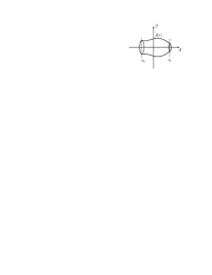
Figure 8: Optimization of the generating function to minimize the moment of inertia of a solid of revolution, the mass is the constraint and the solid lies in the interval $\left[x_{0},x_{f}\right]$ of length $L$.

In all the equations shown in this paper, the MI’s can be seen as functionals of some generating functions. For simplicity, we take a homogeneous solid of complete revolution around the $X-$axis with $f_{1}\left(x\right)=0$. The MI’s are functionals of the remaining generating function, from Eqs. (2.4, 2.7) and relabeling $f_{2}\left(x\right)\equiv f\left(x\right)$, we get

$$I_{X}[f] = \frac{\pi\rho}{2}\int_{x_{0}}^{x_{f}}f\left(x^{\prime}\right)^{4}\ dx^{\prime}\ ,$$ (5.1)

$$I_{Y}[f] = \frac{I_{X}[f]}{2}+\pi\rho\int_{x_{0}}^{x_{f}}x^{\prime 2}f\left(x^{\prime}\right)^{2}\ dx^{\prime}\ .$$ (5.2)

Then, we can use the methods of the calculus of variations (CV) , in order to optimize the MI. To figure out possible applications, imagine that we should build up a figure such that under certain restrictions (that depend on the details of the design) we require a minimum of energy to set the solid at certain angular velocity starting from rest. Thus, the optimal design requires the moment of inertia around the axis of rotation to be a minimum.

As an specific example, suppose that we have a certain amount of material and we wish to make up a solid of revolution of a fixed length with it, such that its MI around a certain axis becomes a minimum. To do it, let us consider a fixed interval $\left[x_{0},x_{f}\right]$ of length $L$, to generate a solid of revolution of mass $M$ and constant density $\rho$ (see Fig. 8). Let us find the function $f\left(x\right)$, such that $I_{X}$ or $I_{Y}$ become a minimum. Since the mass is kept constant, we use it as the fundamental constraint

$$M=\pi\rho\int_{x_{0}}^{x_{f}}f\left(x^{\prime}\right)^{2}\ dx^{\prime}=\text{constant.}$$ (5.3)

In order to minimize $I_{X}$ we should minimize the functional

$$G_{X}\left[f\right]=\int_{x_{0}}^{x_{f}}g\left(f,x^{\prime}\right)\ dx^{\prime}=I_{X}\left[f\right]-\lambda\pi\rho\int_{x_{0}}^{x_{f}}f\left(x^{\prime}\right)^{2}\ dx^{\prime}\ \$$ (5.4)

where $\lambda$ is the Lagrange’s multiplicator associated with the constraint (5.3). In order to minimize $G_{X}\left[f\right]$, we should use the Euler-Lagrange equation [9]

$$\frac{\delta G_{X}[f]}{\delta f(x)}=\frac{\partial g(f,x)}{\partial f}-\frac{\partial}{\partial x}\frac{\partial g(f,x)}{\partial(df/dx)}=0\ \$$ (5.5)

obtaining

$$\frac{\delta G_{X}[f]}{\delta f(x)}=2\pi\rho f\left(x\right)^{3}-2\pi\lambda\rho f\left(x\right)=0\ ,$$ (5.6)

whose non-trivial solution is given by

$$f\left(x\right)=\sqrt{\lambda}\equiv R\ .$$ (5.7)

Analizing the second variational derivative we realize that this condition corresponds to a minimum. Hence, $I_{X}$ becomes minimum under the assumptions above for a cylinder of radius $\sqrt{\lambda}$, such radius can be obtained from the condition (5.3), yielding $R^{2}=M/\pi\rho L$ and $I_{X}$ becomes

$$I_{X,cylinder}=\frac{1}{2}\frac{M^{2}}{\pi\rho L}\ .$$ (5.8)

Now, we look for a function that minimizes the MI of the solid of revolution around an axis perpendicular to the axis of symmetry. From Eqs. (5.2, 5.3), we see that the functional to minimize is

$$G_{Y}[f]=\frac{I_{X}[f]}{2}+\pi\rho\int_{x_{0}}^{x_{f}}x^{\prime 2}f\left(x^{\prime}\right)^{2}\ dx^{\prime}-\lambda\pi\rho\int_{x_{0}}^{x_{f}}f\left(x^{\prime}\right)^{2}\ dx^{\prime}\ ,$$ (5.9)

making the variation of $G_{Y}[f]$ with respect to $f\left(x\right)$ we get

$$f\left(x\right)^{2}=2\left(\lambda-x^{2}\right)\equiv R^{2}-2x^{2}\ ,$$ (5.10)

where we have written $2$$\lambda=R^{2}$. By taking $x_{0}=-L/2,\ x_{f}=L/2$, the function obtained is an ellipse centered at the origin with semimajor axis $R\$along the $Y-$axis, semiminor axis $R/\sqrt{2}\$along the $X-$axis, and with eccentricity $\varepsilon=1/\sqrt{2}$. When it is revolved we get an ellipsoid of revolution (spheroid); such spheroid is the solid of revolution that minimizes the MI with respect to an axis perpendicular to the axis of revolution. From the condition (5.3) we find

$$R^{2}=\frac{M}{\pi\rho L}+\frac{L^{2}}{6}\ .$$ (5.11)

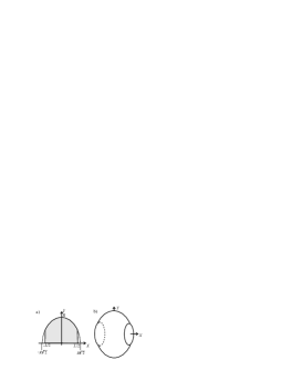
Figure 9: (a) Elliptical function that generates the solids of revolution that minimize$\ I_{Y}$. The shaded region is the one that generates the solid. (b) Truncated spheroid obtained when the shaded region is revolved.

In the most general case, the spheroid generated this way is truncated, as it is shown in Fig. 9, and the condition $R\geq L/\sqrt{{2}}$ should be fulfilled for $f\left(x\right)$ to be real. The spheroid is complete when $R=L/\sqrt{{2}}$, and the mass obtained in this case is the minimum one for the spheroid to fill up the interval $[-L/2,L/2]$, this minimum mass is given by

$$M_{\min}=\frac{\pi\rho L^{3}}{3}\ ,$$ (5.12)

from (5.2), (5.10), (5.11) and (5.12) we find

$$I_{Y,spheroid}=\frac{M_{\min}L^{2}\left[5\mu+5\mu^{2}-1\right]}{60}\ ;\ \mu\equiv\frac{M}{M_{\min}}.$$ (5.13)

Assuming that the densities and masses of the spheroid and the cylinder coincide, we estimate the quotients

$$\frac{I_{Y,cylinder}}{I_{Y,spheroid}} =\frac{\left(5\mu+5\mu^{2}-1\right)}{5\mu\left(\mu+1\right)}<1,$$

$$\frac{I_{X,cylinder}}{I_{X,spheroid}} =\left(1+\frac{1}{5}\mu^{-2}\right)^{-1}<1\ \ .$$ (5.14)

Eqs. (5.14) show that $I_{Y,sph}<I_{Y,cyl}$ while $I_{X,cyl}<I_{X,sph}$. In both cases if $M>>M_{\min}$ the MI’s of the spheroid and the cylinder coincide, it is because the truncated spheroid approaches the form of a cylinder when the amount of mass to be distributed in the interval of length $L$ is increased.

On the other hand, in many applications what really matters are the MI’s around axes passing through the CM. In the case of homogeneous solids of revolution the axis that generates the solid passes through the CM, but this is not necessarily the case for an axis perpendicular to the former. If we are interested in minimizing $I_{Y_{C}}$, i.e. the MI with respect to an axis parallel to $Y$ and passing through the CM, we should write the expression for $I_{Y_{C}}\$by using the parallel axis theorem and by combining Eqs. (5.2, 5.3, A.2)

$$I_{Y_{C}}[f] =\frac{I_{X}[f]}{2}+\pi\rho\int_{x_{0}}^{x_{f}}x^{\prime 2}f\left(x^{\prime}\right)^{2}\ dx^{\prime}$$

$$-\frac{\pi\rho}{\int_{x_{0}}^{x_{f}}f\left(x^{\prime}\right)^{2}dx^{\prime}}\left[\int_{x_{0}}^{x_{f}}x^{\prime}f(x^{\prime})^{2}\ dx^{\prime}\right]^{2}\ ,$$ (5.15)

thus, the functional to be minimized is

$$G_{Y_{C}}\left[f\right]=I_{Y_{C}}[f]-\lambda\pi\rho\int_{x_{0}}^{x_{f}}f\left(x^{\prime}\right)^{2}\ dx^{\prime}\ ,$$ (5.16)

after some algebra, we arrive to the following minimizing function

$$f\left(x\right)^{2}=R^{2}-2\left(x-x_{CM}\right)^{2}\ ,$$ (5.17)

where we have written $2\lambda=R^{2}$. It corresponds to a spheroid (truncated, in general) centered at the point $\left(x_{CM},0,0\right)$ as expected, showing the consistency of the method.

Finally, it worths remarking that the techniques of the CV shown here can be extrapolated to more complex situations, as long as we are able to see the MI’s as functionals of certain generating functions. The situations shown here are simple for pedagogical reasons, but they open a window for other applications with other constraints,  for which the minimization cannot be done by intuition. For instance, if our constraint consists of keeping the surface constant, the solutions are not easy to guess, and should be developed by variational methods.

6 Analysis and conclusions

Most textbooks report MI’s for only a few number of simple figures. By contrast, the examples illustrated in this work have been chosen to be more general, and can also cover many particular cases. On the other hand, in the specific case of solids of revolution, only the MI with respect to the symmetry axis is usually reported. Perhaps the most advantageous feature of the methods developed in this paper is that the three moments of inertia $I_{X},I_{Y},I_{Z}$ can be calculated by applying the same limits of integration, and we do not have to worry about the partitions. It is because all three moments of inertia are written in terms of the generating functions of the solid. For instance, any solid of revolution acting as a physical pendulum provides an example in which the MI with respect to an axis perpendicular to the axis of symmetry is necessary, an specific case is example 8 for the Gaussian bell (see appendix B.1). Moreover, we examine the conditions for the perpendicular MI’s to be degenerate, we find that this degeneracy occurs even for inhomogeneous solids as long as the density has an azimuthal symmetry. Remarkably, even for incomplete solids of revolution with the azimuthal symmetry broken, such degeneracy may occur under certain conditions.

Finally, we point out that for solids of revolution in which densities depend only on the height of the solid, the expressions for the MI become simple integrals, such fact makes the integration process much easier. Simple integrals are advantageous even in the case in which we cannot evaluate them analytically. Numerical methods to evaluate MI’s utilize typically the geometrical shape of the body; instead, numerical methods for simple integrals are usually easier to manage.

As for the technique of contour plots, we can realize that many different figures could have the same type of contours though a different modulation of them, one specific example is the case of a cone with elliptical cross section and a general ellipsoid, in both solids the contours are ellipses but they are modulated (scaled with the $z$ coordinate) in different ways. On the other hand, in some cases the contours are different but the modulation is of the same type, for example a cone and a pyramid has the same type of modulation (scaling) but their contours are totally different. In both situations we can save a lot of effort by making profit from the similarities. The reader can check the examples 4, 5 and 6, in order to figure out the way in which we can exploit these symmetries in practical calculations.

Furthermore, textbooks always consider homogeneous figures to estimate the MI, assumption that is not always realistic. As for our formulae, though they simplify considerably when we consider homogeneous bodies, the methods are tractable in many cases when inhomogeneous objects are considered, allowing more realistic results.

Another interesting remark is that these methods can be used to calculate products of inertia in the case in which the complete tensor of inertia is necessary. Moreover, expressions for the CM proceed by similar arguments, and the appendix A, shows some formulae for the CM of solids of revolution and solids built up by contour plots. In such expressions we realize that the same limits of integration defined for the calculation of the MI’s are used to calculate the CM.

Finally, since all our formulae for MI’s depend on certain generating functions, we can see the MI of a wide variety of figures as a functional, making the MI’s suitable to utilize methods of the calculus of variations. In particular, minimization of the MI under certain restrictions is possible utilizing variational methods, it could be very useful in applied physics and engineering.

The authors acknowledge to Dr. Héctor Múnera for revising the manuscript.

Appendix A Calculation of centers of mass

A.1 CM of solids of revolution generated around the $X-axis$

Taking into account the definition of the center of mass for continuous systems

$$\vec{r}_{CM}=\frac{\int\vec{r}\ dm}{\int dm}\ ,$$

we can get general formulae to calculate the CM of a solid by using a similar procedure to the one followed to get MI’s. First of all we calculate the total mass based on the density and the geometrical shape of the body. In the case of solids of revolution around the $X-$axis, the total mass of the solid is given by

$$M=\int dm=\int_{x_{0}}^{x_{f}}\left\{\int_{f_{1}\left(x\right)}^{f_{2}\left(x\right)}\left[\int_{\theta_{0}}^{\theta_{f}}\rho\left(x,r_{x},\theta\right)\ d\theta\right]r_{x}\ dr_{x}\right\}\ dx\ ,$$ (A.1)

and the CM coordinates read

$$X_{CM} = \frac{1}{M}\int_{x_{0}}^{x_{f}}\left\{\int_{f_{1}\left(x\right)}^{f_{2}\left(x\right)}\left[\int_{\theta_{0}}^{\theta_{f}}\rho\left(x,r_{x},\theta\right)\ d\theta\right]r_{x}\ dr_{x}\right\}x\ dx\ ,$$ (A.2)

$$Y_{CM} = \frac{1}{M}\int_{x_{0}}^{x_{f}}\left\{\int_{f_{1}\left(x\right)}^{f_{2}\left(x\right)}\left[\int_{\theta_{0}}^{\theta_{f}}\rho\left(x,r_{x},\theta\right)\cos\theta\ d\theta\right]r_{x}^{2}\ dr_{x}\right\}\ dx\ ,$$ (A.3)

$$Z_{CM} = \frac{1}{M}\int_{x_{0}}^{x_{f}}\left\{\int_{f_{1}\left(x\right)}^{f_{2}\left(x\right)}\left[\int_{\theta_{0}}^{\theta_{f}}\rho\left(x,r_{x},\theta\right)\sin\theta\ d\theta\right]r_{x}^{2}\ dr_{x}\right\}\ dx\ ,$$ (A.4)

the limits of integrations are the ones defined in Sec. 2.1. In the case of complete revolution with $\rho=\rho\left(x,r_{x}\right)$, we obtain $Y_{CM}=Z_{CM}=0$, as expected from the cylindrical symmetry.

A.2 CM of solids of revolution generated around the $Y-axis$

By using the coordinate system and the limits of integration defined in Sec. 3, we can evaluate the CM for solids of revolution generated around the $Y-$axis obtaining

$$X_{CM} = \frac{1}{M}\int_{x_{0}}^{x_{f}}\left\{\int_{f_{1}\left(r_{y}\right)}^{f_{2}\left(r_{y}\right)}\left[\int_{\phi_{0}}^{\phi_{f}}\sin(\phi)\rho\left(r_{y},y,\phi\right)\ d\phi\right]\ dy\right\}r_{y}^{2}\ dr_{y}\ ,$$ (A.5)

$$Y_{CM} = \frac{1}{M}\int_{x_{0}}^{x_{f}}\left\{\int_{f_{1}\left(r_{y}\right)}^{f_{2}\left(r_{y}\right)}\left[\int_{\phi_{0}}^{\phi_{f}}\rho\left(r_{y},y,\phi\right)\ d\phi\right]\ y\ dy\right\}r_{y}\ dr_{y}\ ,$$ (A.6)

$$Z_{CM} = \frac{1}{M}\int_{x_{0}}^{x_{f}}\left\{\int_{f_{1}\left(r_{y}\right)}^{f_{2}\left(r_{y}\right)}\left[\int_{\phi_{0}}^{\phi_{f}}\rho\left(r_{y},y,\phi\right)\cos(\phi)\ d\phi\right]\ dy\right\}r_{y}^{2}\ dr_{y}\ ,$$ (A.7)

$$M = \int_{x_{0}}^{x_{f}}\left\{\int_{f_{1}\left(r_{y}\right)}^{f_{2}\left(r_{y}\right)}\left[\int_{\phi_{0}}^{\phi_{f}}\rho\left(r_{y},y,\phi\right)\ d\phi\right]\ dy\right\}r_{y}\ dr_{y}\ .$$ (A.8)

In the case of a complete revolution with $\rho=\rho\left(r_{y},y\right)$, we get $X_{CM}=Z_{CM}=0$, due to the cylindrical symmetry.

A.3 CM of solids formed by contour plots

In this case, we use the limits of integration defined in Sec. 4. The CM coordinates read

$$x_{CM} = \frac{1}{M}\int_{z_{0}}^{z_{f}}\left\{\int_{x_{0}\left(z\right)}^{x_{f}\left(z\right)}\left[\int_{f_{1}\left(x,z\right)}^{f_{2}\left(x,z\right)}\rho\left(x,y,z\right)\ dy\right]x\ dx\right\}dz\ ,$$ (A.9)

$$y_{CM} = \frac{1}{M}\int_{z_{0}}^{z_{f}}\left\{\int_{x_{0}\left(z\right)}^{x_{f}\left(z\right)}\left[\int_{f_{1}\left(x,z\right)}^{f_{2}\left(x,z\right)}\rho\left(x,y,z\right)\ y\ dy\right]\ dx\right\}dz\ ,$$ (A.10)

$$z_{CM} = \frac{1}{M}\int_{z_{0}}^{z_{f}}\left\{\int_{x_{0}\left(z\right)}^{x_{f}\left(z\right)}\left[\int_{f_{1}\left(x,z\right)}^{f_{2}\left(x,z\right)}\rho\left(x,y,z\right)\ dy\right]\ dx\right\}z\ dz\ ,$$ (A.11)

$$M = \int_{z_{0}}^{z_{f}}\left\{\int_{x_{0}\left(z\right)}^{x_{f}\left(z\right)}\left[\int_{f_{1}\left(x,z\right)}^{f_{2}\left(x,z\right)}\rho\left(x,y,z\right)\ dy\right]\ dx\right\}dz\ .$$ (A.12)

Appendix B Some additional examples for the calculation of moments of inertia

In this appendix we carry out additional calculations of moments of inertia for some specific figures, by applying the formulae written in sections 2, 3 and 4; in order to illustrate the power of the methods.

B.1 Examples of moments of inertia for solids of revolution

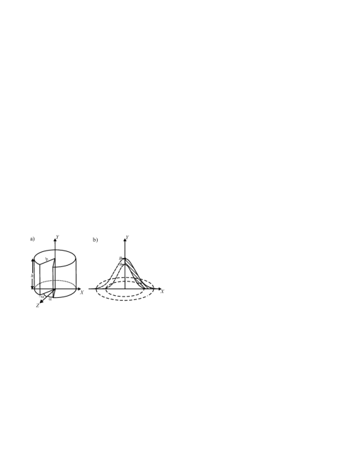
Figure 10: On left: cylindrical wedge generated around the $Y-$axis. On right: A bell modelated by two Gauss’ distributions rotating around the $Y-$axis, the bell tolls around an axis perpendicular to the sheet that passes through the point $B$

Example 7

MI for a cylindrical wedge (see Fig. 10). Let us consider a cylinder of height $h$ and radius $b$, whose density is given by

$$\rho(\phi)=\left\{\begin{array}[]{c}\rho\text{, \ }\alpha\leq\phi\leq 2\pi-\alpha\\[2.84526pt] 0\text{, \ }-\alpha<\phi<\alpha\end{array}\right.$$

and that is generated around the $Y-$axis by means of the functions$\ f_{1}\left(x\right)=0$ and $\ f_{2}\left(x\right)=h$. From Eq. (A.8) and Eqs.(3.1-3.3) we find

$$M=(\pi-\alpha)\rho hb^{2}\ ,$$

$$I_{X}=M\left[\frac{b^{2}}{8}\left(2-\frac{\sin 2\alpha}{(\pi-\alpha)}\right)+\frac{h^{2}}{3}\right]\ ;\ I_{Y}=\frac{Mb^{2}}{2}\ ;\ I_{Z}=M\left[\frac{b^{2}}{8}\left(2+\frac{\sin 2\alpha}{(\pi-\alpha)}\right)+\frac{h^{2}}{3}\right]\ .$$

In order to calculate the moments of inertia from axes passing through the center of mass we use Eqs. (A.5-A.7) to get

$$X_{CM}=0\text{\ };\text{\ }Y_{CM}=\frac{h}{2}\ ;\ Z_{CM}=-\frac{2}{3}\frac{b}{(\pi-\alpha)}\sin\alpha.$$

Example 8

MI’s for a Gaussian Bell. Let us consider a homogeneous hollow bell, which can be reasonably described by a couple of Gaussian distributions (see Fig. 10).

$$f_{1}(x)=Ae^{-\alpha x^{2}}\ ;\ f_{2}(x)=Be^{-\beta x^{2}}\ ,$$

where $\alpha,\beta,A,B$ are positive numbers, $A<B$, and $\alpha>\beta$. The MI’s are obtained from (3.6, 3.7)

$$I_{Y}=\pi\rho\left[\frac{B}{\beta^{2}}-\frac{A}{\alpha^{2}}\right]\ \ ;\ \ I_{X}=I_{Z}=\frac{\pi\rho}{2}\left[\frac{B}{\beta^{2}}-\frac{A}{\alpha^{2}}\right]+\frac{\pi\rho}{9}\left[\frac{B^{3}}{\beta}-\frac{A^{3}}{\alpha}\right]$$

Besides, the mass and the center of mass position read

$$M=\pi\rho\left[\frac{B}{\beta}-\frac{A}{\alpha}\right]\ \ ;\ \ Y_{CM}=\frac{1}{4}\left[\frac{\alpha B^{2}-\beta A^{2}}{\alpha B-\beta A}\right]\ ;\ X_{CM}=Z_{CM}=0\ .$$

When the bell tolls, it rotates around an axis perpendicular to the axis of symmetry that passes the top of the bell. Thus, this is a real situation in which the perpendicular MI is required. On the other hand, owing to the cylindrical symmetry, we can calculate this moment of inertia by taking any axis parallel to the $X-$axis. In our case the top of the bell corresponds to$\ y=B$, and using Steiner’s theorem it can be shown that

$$I_{X,B} = I_{X}+MB(B-2Y_{CM})$$

$$I_{X,B} = \frac{\pi\rho}{18\alpha^{2}\beta^{2}}\left[\alpha^{2}B(9+11B^{2}\beta)+\beta^{2}A(9AB\alpha-2A^{2}\alpha-18B^{2}\alpha-9)\right]\ .$$

B.2 Examples of MI’s by the method of contourplots

Example 9

A thin elliptical plate: for this bidimensional object, we can use Eqs. (4.5, 4.6), the delimited function can be taken from (4.7) but with $z=0$. The results are

$$I_{X} = M\frac{b^{2}}{4}\ \ ;\ \ I_{Y}=M\frac{a^{2}}{4}\ ,$$

$$I_{Z} = M\frac{\left(a^{2}+b^{2}\right)}{4}\ \ ;\ \ M=\pi\sigma ab\ .$$

once again, these axes passes through the center of mass of the figure.

Figure 11: Arbitrary quadrilateral, the dimensions are indicated in the drawing.

Example 10

An arbitrary quadrilateral, (see Fig. 11): This is a bidimensional figure, so we apply Eqs. (4.5, 4.6). The bounding functions are given by

$$f_{1}\left(x\right)=0\ ,$$

$$f_{2}\left(x\right)=\left\{\begin{array}[]{ccc}\frac{h_{1}}{a_{1}}x&if&0\leq x\leq a_{1}\\[5.69054pt] \frac{\left(h_{2}-h_{1}\right)}{a_{2}}x+\frac{h_{1}\left(a_{1}+a_{2}\right)-h_{2}a_{1}}{a_{2}}&if&a_{1}<x\leq a_{1}+a_{2}\\[5.69054pt] -\frac{h_{2}}{a_{3}}x+\frac{h_{2}}{a_{3}}\left(a_{1}+a_{2}+a_{3}\right)&if&a_{1}+a_{2}<x\leq a_{1}+a_{2}+a_{3}\end{array}\right.$$

and the moments of inertia read

$$I_{X}=\frac{\sigma}{12}\left[a_{2}\left(h_{1}+h_{2}\right)\left(h_{1}^{2}+h_{2}^{2}\right)+h_{1}^{3}a_{1}+h_{2}^{3}a_{3}\right]\allowbreak$$ (B.1)

$$I_{Y} = \allowbreak\frac{\sigma}{12}\left[12a_{1}a_{2}a_{3}h_{2}+\left(4a_{1}a_{2}^{2}+3a_{1}^{3}+a_{2}^{3}\right)h_{1}+\left(4a_{2}a_{3}^{2}+3a_{2}^{3}+a_{3}^{3}\right)h_{2}\right.$$ (B.2)

$$\left.+6a_{1}^{2}a_{2}\left(h_{1}+h_{2}\right)+4a_{1}h_{2}\left(2a_{2}^{2}+a_{3}^{2}\right)+6a_{3}h_{2}\left(a_{1}^{2}+a_{2}^{2}\right)\right]$$

$$I_{Z}=I_{X}+I_{Y}$$ (B.3)

the center of mass coordinates are given by

$$x_{CM} = \frac{\allowbreak\sigma}{6M}\left[3a_{1}a_{2}\left(h_{1}+h_{2}\right)+3a_{3}h_{2}\left(a_{1}+a_{2}\right)\right.$$ (B.4)

$$\left.+h_{1}\left(2a_{1}^{2}+a_{2}^{2}\right)+h_{2}\left(2a_{2}^{2}+a_{3}^{2}\right)\right]$$

$$y_{CM}=\frac{\sigma}{6M}\left[a_{2}h_{1}h_{2}+\left(a_{1}+a_{2}\right)h_{1}^{2}+\left(a_{2}+a_{3}\right)h_{2}^{2}\right]\allowbreak$$ (B.5)

with

$$M=\frac{\sigma}{2}\left[a_{1}h_{1}+a_{2}\left(h_{1}+h_{2}\right)+a_{3}h_{2}\right]$$ (B.6)

The quantities $I_{X},~{}y_{CM},$ and$\ M$; are invariant under traslations in $x$, for example $I_{X}$ might be calculated as

$$I_{X}=\frac{\sigma}{3}\int_{x_{0}}^{x_{f}}f_{2}\left(x\right)^{3}dx=\frac{\sigma}{3}\int_{x_{0}-\Delta x}^{x_{f}-\Delta x}f_{2}\left(u+\Delta x\right)^{3}du$$

where we have performed a traslation $\Delta x$ to the left. It is equivalent to make the change of variables $u=x-\Delta x$. This property can be used to evaluate the integrals easier. Specifically, the piece of Fig. 11 lying in the interval $a_{1}<x\leq a_{1}+a_{2}$, can be traslated to the origin by using $\Delta x=a_{1}$; and the piece of this figure lying at $a_{1}+a_{2}<x\leq a_{1}+a_{2}+a_{3}$ can be also traslated to the origin with $\Delta x=a_{1}+a_{2}$. On the other hand, though the quantities $I_{Y}$ and $x_{CM}$ are not invariant under such traslations, the same change of variables simplifies their calculations. This strategy is very useful in solids or surfaces that can be decomposed by pieces (i.e. when at least one of the generator functions is defined by pieces). For example, the same change of variables could be used if we are interested in the solid of revolution generated by the surface of Fig. 11.

Finally, from Eqs. (B.1-B.6) we can obtain many particular cases, some of them are

• $h_{1}=h_{2}$ trapezoid.

• $a_{1}=h_{1}=0$ arbitrary triangle.

• $a_{2}=0,\ a_{1}=a_{3}=\frac{h_{1}}{\sqrt{3}}=\frac{h_{2}}{\sqrt{3}}\equiv\frac{L}{2}$ equilateral triangle of side length $L$.

• $a_{1}=h_{1}=0,\ a_{2}=a_{3}=\frac{h_{2}}{\sqrt{3}}\equiv\frac{L}{2}$ equilateral triangle of side length $L$.

• $a_{1}=a_{3}=h_{1}=0$ triangle with a right angle.

• $h_{2}=h_{1},$ $a_{2}=0$ arbitrary triangle.

• $a_{1}=a_{3}=0,\ h_{2}=h_{1}$ rectangle.

Appendix C Table of moments of inertia

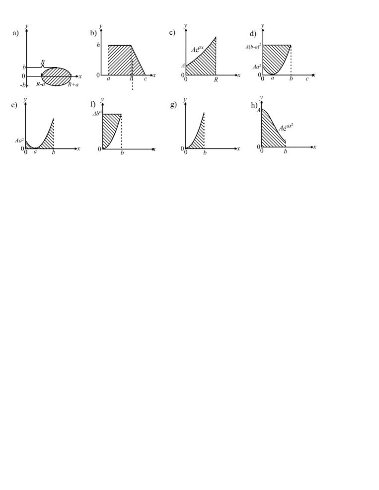
Figure 12: Surfaces that generates the solids whose moments of inertia appears on the table 1

In table 1 on page 1, the moments of inertia for a variety of solids of revolution generated around the $Y-$axis are displayed, such table includes the function generators and any other information necessary to carry out the calculations by means of our methods. The surfaces that generates the solids are displayed in Fig. 12. Observe that the first of these surfaces generates a torus with elliptical cross section and the second one generates a truncated hollow cone.

Finally, there are some conditions for certain parameters of these figures. In Fig. (d), $a>0$, and $b>2a$; in Fig. (e) $b>0$, and $a>0$, in Fig. (f), $n>0$; for Fig. (g), $n>-2/3$; in Figs. (c) and (h) $a$ can also be negative.

Fig $f_{1}(x)$ $f_{2}(x)$ $x_{0}$ $x_{f}$ $M$ $I_{Y}$ $I_{X}=I_{Z}$ $Y_{CM}$ a $-f_{2}(x)$ $\frac{b\sqrt{a^{2}-(x-R)^{2}}}{a}$ $R-a$ $R+a$ $2\pi^{2}\rho Rba$ $M(R^{2}+\frac{3}{4}a^{2})$ $\frac{M}{8}(4R^{2}+3a^{2}+2b^{2})$ $0$ b $0$ $h,a<x<b$ $h\frac{c-x}{c-b},b\leq x\leq c$ $a$ $c$ $\frac{\pi\rho h}{3}(b^{2}+bc$ $+c^{2}-3a^{2})$ $\frac{\pi\rho h}{10}[b^{4}+b^{3}c+b^{2}c^{2}$ $+bc^{3}+c^{4}-5a^{4}]$ $\frac{I_{y}}{2}+\pi\rho h^{3}\times$ $\frac{\left(3bc+6b^{2}+c^{2}-10a^{2}\right)}{30}$ $\frac{h}{4}\frac{\left(3b^{2}+2bc+c^{2}-6a^{2}\right)}{[b^{2}+bc+c^{2}-3a^{2}]}$ c $0$ $Ae^{ax}$ $0$ $b$ $\frac{2\pi A\rho}{a^{2}}\left(e^{ab}ab\right.$ $\left.-e^{ab}+1\right)$ $\frac{2\pi A\rho}{a^{4}}e^{ab}\left(a^{3}b^{3}-3a^{2}b^{2}\right.$ $\left.+6\left(ab-1+e^{-ab}\right)\right)$ $\frac{1}{2}I_{Y}+\frac{2\pi}{27a^{2}}\rho A^{3}\times$ $\left(e^{3ab}\left(3ab-1\right)+1\right)$ $\frac{A}{8}\frac{\left(e^{2ab}\left(2ab-1\right)+1\right)}{\left(e^{ab}\left(ab-1\right)+1\right)}$ d $A(x-a)^{2}$ $A(b-a)^{2}$ $0$ $b$ $\allowbreak\frac{\pi A\rho b^{3}}{6}\left(3b-4a\right)$ $M\frac{b^{2}}{5}(\frac{5b-6a}{3b-4a})$ $\frac{I_{y}}{2}+\frac{b^{3}\rho A^{3}\pi}{84}(21b^{5}$ $-120ab^{4}+280a^{2}b^{3}$ $-336a^{3}b^{2}+210a^{4}b-56a^{5})$ $\frac{A\left(10b^{3}+45a^{2}b-36ab^{2}-20a^{3}\right)}{5\left(3b-4a\right)}$ e $0$ $A(x-a)^{2}$ $0$ $b$ $\frac{1}{6}\pi\rho Ab^{2}(3b^{2}$ $-8ab+6a^{2})$ $\frac{\pi\rho b^{4}A}{30}(10b^{2}$ $-24ab+15a^{2})$ $\frac{I_{y}}{2}+\frac{b^{2}\rho A^{3}\pi}{84}\left[28a^{6}+7b^{6}-\right.$ $48ab^{5}-112a^{5}b+140a^{2}b^{4}$ $\left.-224a^{3}b^{3}+210a^{4}b^{2}\right]$ $\frac{A}{5}(15a^{4}+5b^{4}-24ab^{3}$ $-40a^{3}b+45a^{2}b^{2})\times$ $\frac{1}{\left(3b^{2}-8ab+6a^{2}\right)}$ f $Ax^{n}$ $Ab^{n}$ $0$ $b$ $\pi\rho Ab^{n+2}\frac{n}{n+2}$ $M\frac{b^{2}}{2}\frac{n+2}{n+4}$ $\frac{I_{y}}{2}+MA^{2}b^{2n}\frac{n+2}{3n+2}$ $A\frac{n+2}{2n+2}b^{n}$ g $0$ $Ax^{n}$ $0$ $b$ $2\pi\rho A\frac{b^{n+2}}{n+2}$ $Mb^{2}\frac{n+2}{n+4}$ $\frac{I_{y}}{2}+\frac{1}{3}M\frac{n+2}{3n+2}A^{2}b^{2n}$ $\frac{A}{4}\frac{b^{n}(n+2)}{n+1}$ h $0$ $Ae^{-ax^{2}}$ $0$ $b$ $\pi\rho A\frac{1-e^{-b^{2}a}}{a}$ $M\frac{1-e^{-ab^{2}}(1-ab^{2})}{a(1-e^{-ab^{2}})}$ $\frac{I_{Y}}{2}+\frac{MA^{2}(1+e^{-ab^{2}}+e^{-2ab^{2}})}{9}$ $\frac{A}{4}\frac{(1-e^{-2ab^{2}})}{(1-e^{-ab^{2}})}$

Table 1: Moments of inertia for a variety of solids of revolution generated around the $Y-$ axis, the surfaces that generates the solids are displayed in Fig. 12

References

• [1] D. Kleppner and R. Kolenkow, An introduction to mechanics (McGRAW-HILL KOGAKUSHA LTD, 1973); R. Resnick and D. Halliday, Physics (Wiley, New York, 1977), 3rd Ed.; M. Alonso and E. Finn, Fundamental University Physics, Vol I, Mechanics (Addison-Wesley Publishing Co., Massachussets, 1967).
• [2] R. C. Hibbeler, Engineering Mechanics Statics, Seventh Ed. (Prentice-Hall Inc., New York,1995).
• [3] Louis Leithold, The Calculus with Analytic Geometry (Harper & Row, Publishers, Inc. , New York, 1972), Second Ed.; E. W. Swokowski, Calculus with Analytic Geometry (PWS-KENT Publishing Co., Boston Massachusetts, 1988), Fourth Ed.; S. K. Stein, Calculus and Analytic Geometry (Mc-Graw Hill Book Co. 1987), Fourth Ed.
• [4] R. Szmytkowski, “Simple method of calculation of moments of inertia”, Am. J. Phys. 56, 754-756 (1988); R. Rabinoff “Moments of inertia by scaling arguments: How to avoid messy integrals” Am. J. Phys. 53, 501-502 (1985).
• [5] Carl M. Bender and Lawrence R. Mead, “D-dimensional moments of inertia” Am. J. Phys. 63, 1011-1014 (1995); J. Casey and S. Krishnaswamy, “Problem: Which rigid bodies have constant inertia tensors?” Am. J. Phys. 63, 276-281 (1995); P. K. Aravind, “A comment on the moment of inertia of symmetrical solids” Am. J. Phys. 60, 754-755 (1992); P. K. Aravind, “Gravitational collapse and moment of inertia of regular polyhedral configurations” Am. J. Phys. 59, 647-652 (1991); J. Satterly, “Moments of Inertia of Solid Rectangular Parallelopipeds, Cubes, and Twin Cubes, and Two Other Regular Polyhedra” Am. J. Phys. 25, 70-78 (1957) ; J. Satterly, “Moments of Inertia of Plane Triangles” Am. J. Phys. 26, 452-453 (1958).
• [6] W. N. Mei and Dan Wilkins, “Making a pitch for the center of mass and the moment of inertia” Am. J. Phys. 65, 903-907 (1997); Joseph C. Amato and Roger E. Williams and Hugh Helm, “A black box moment of inertia apparatus” Am. J. Phys. 63, 891-894 (1995).
• [7] J. F. Streib, “A theorem on moments of inertia” Am. J. Phys. 57, 181 (1989).
• [8] Rodolfo A. Diaz, William J. Herrera, R. Martinez, http://xxx.lanl.gov/list/physics/0507  Preprint number: physics/0507172.
• [9] G. Arfken. Mathematical methods for physicists, Second Ed. (Academic Press, International Edition, 1970) Chap. 17.