1s2s2p²3d ⁶L - 1s2p³3d ⁶D, L=F, D, P Transitions in O IV, F V and Ne VI

Abstract

We present observations of VUV transitions between doubly excited sextet states in O IV, F V and Ne VI. Spectra were produced by collisions of an O⁺ beam with a solid carbon target. We also studied spectra obtained previously of F V and Ne VI. Some observed lines were assigned to the 1s2s2p²3d ⁶L - 1s2p³3d ⁶D, L=F, D, P electric-dipole transitions, and compared with results of MCHF (with QED and higher-order corrections) and MCDF calculations. 42 new lines have been identified. Highly excited sextet states in five-electron ions provide a new form of energy storage and are possible candidates for VUV and x-ray lasers.

I Introduction

Highly excited sextet states in five-electron ions provide a form of energy storage. The research for stimulated VUV- and x-ray emission from highly excited sextet states in five-electron ions has attracted attention in recent years. This new form of energy storage and potential VUV-ray lasers could have many applications in basic science, technology, medicine, and defense. In a proposed VUV and x-ray laser system, one seeks a probability to trigger a release of K- and L-hole energies of sextet states in boron-like ions. Although K- and L-hole energies are not as high as energies released in nuclear fusion, capacity of highly excited sextet states in five-electron ions to store energy is significant (several hundred electron volts per atom shown in Fig. 1). Such a system involves long-lived ”storage” metastable states, and there nearby are short-lived higher excited sextet states, from which transitions are emitted with photon radiation, and quintet continuum. An ideal system where VUV and x-ray lasers may be implemented would be among heavy and highly excited ions that have metastbale sextet states with long lifetimes. However, structure and transition properties of these sextet states are currently very poorly known.

Figure 1: Term diagram of doubly excited sextet states of O IV. The mean wavelength for the 1s2s2p²3d ⁶L-1s2p³3d ⁶D^o transitions in O IV is shown.

In 1992 beam-foil spectroscopy Blanke et al (1992); Lapierre and Knystautas (2000) was used to provide initial data on low-lying sextet states in doubly excited boron-like nitrogen, oxygen and fluorine. Recent work of Lapierre and Knystautas Lapierre and Knystautas (2000) on possible sextet transitions in Ne VI highlights the significance in this sequence. They measured several excitation energies and lifetimes. Fine structures of individual 1s2s2p²3s ⁶P_J states were resolved and measured in O IV, F V and Ne VI by Lin and Berry et al Lin and berry  et al (2003). There are no further results reported for transitions from highly excited sextet states.

In his work, fast beam-foil spectra of oxygen were recorded at Liege using grading incidence spectrometers Berry  et al (1975); Kramida  et al (1999). Spectra of fluorine and neon were previously recorded at the University of Lyon and the Argonne National Lab, The 1s2s2p²3d ⁶L - 1s2p³3d ⁶D, L=F, D, P electric-dipole transitions in O IV, F V and Ne VI have been searched in these spectra, and compared with results of MCHF (with QED and higher-order corrections) and MCDF calculations.

II THEORY

Energies, lifetimes and relevant E1 transition rates of the doubly excited sextet states 1s2s2p²3d ⁶L, L=F, D, P and 1s2p³3d ⁶D in boron-like O IV, F V and Ne VI were calculated with Multi-configuration Hartree-Fock (MCHF) method Miecznik  et al (2000); Fischer  et al (2000) (with QED and higher-order relativistic corrections Lin and berry  et al (2003); Chung  et al (1992)), and Multi-configuration Dirac-Fock (MCDF) GRASP code Dyall &  Grant  et al (1989); Parpia, Fischer and Grant (1996); Fritzsche and Grant &  Grant  et al (1997).

For a sextet state in a five-electron system (ß, LS=5/2JM_J)=(n₁l${}_{1}^{w1}$n₂l${}_{2}^{w2}$ n₃l${}_{3}^{w3}$ n₄l${}_{4}^{w4}$ n₅l${}_{5}^{w5}$ ⁶L_J, M_J ), where wi=0,1, …, or min (2l_i+1), i=1,2,… 5, the wavefunction is

$$\Psi(\beta,LS=5/2J)=\sum\limits_{i=1}^{N}\sum\limits_{M_{J}=-J}^{J}c_{i}\phi(\beta_{i},LS=5/2JM_{J}),$$ (1)

where c_i is a configuration interaction coefficient, N is a total number of configurations with the same LSJM_J and parity, and $\phi$(ß_i,LS=5/2JM_J) is a configuration state function (CSF).

In single-configuration Hartree-Fock (SCHF) calculations only the configurations corresponding to the desired levels, 1s2s2p²3d or 1s2p³3d, were considered. After updating MCHF codes we performed relativistic calculations with an initial expansion of up to 4000 CSFs and a full Pauli-Breit Hamiltonian matrix. For a five-electron system a CI expansion generated by an active set leads to a large number of expansions. To reduce the number of configurations, we chose configurations n₁l₁n₂l₂ n₃l₃ n₄l₄ n₅l₅, where n_i=1, 2, 3, 4 and 5, l_i=0, …min (4, n_i-1). We did not include g electrons for n=5 shell. For MCHF calculations of the lower states 1s2s2p²3d ⁶L, L=F, D, P we chose 1s, 2s, 2p, 3s, 3p, 3d, 4s, 4p, 4d and 5s electrons to compose configurations. For the 1s2p³3d ⁶D state we chose 1s through 4d electrons. Fine structure splitting is strongly involved in the experiments and identifications. After determining radial wavefunctions we included relativistic operators of mass correction, one- and two-body Darwin terms and spin-spin contact term in both SCHF and MCHF calculations; these were not included by Miecznik et al Miecznik  et al (2000).

We used the screened hydrogenic formula from Lin and berry  et al (2003); Chung  et al (1992, 1993); Drake and Swainson (1990) to estimate quantum electrodynamic effects (QED) and higher-order relativistic contributions for sextet states in five-electron oxygen, fluorine and neon.

In MCDF Dyall &  Grant  et al (1989); Parpia, Fischer and Grant (1996); Fritzsche and Grant &  Grant  et al (1997) calculations, firstly we used single-configuration Dirac-Fock approach (SCDF). A basis of jj-coupled states to all possible total angular momenta J from two non-relativistic configurations, 1s2s2p²3d and 1s2p³3d, was considered. For convergence we included the ground state 1s²2s²2p of the five-electron systems. After calculating all possible levels for all J, eigenvectors were regrouped in a basis of LS terms. To obtain better evaluations of correlation energies of the doubly excited sextet terms 1s2s2p²3d ⁶L, L=F, D, P and 1s2p³3d ⁶D in O IV, F V and Ne VI, improved calculations included 1s²2s²2p, 1s²2s2p², 1s2s²2p², 1s2s2p³, 1s2s2p²3s, 1s2s2p²3p, 1s2s2p²3d, 1s2p³3s, 1s2p³3p, 1s2p³3d, 1s2p³4s, 1s2p³4p and 1s2p³4d mixing non-relativistic configurations.

In GRASP code Dyall &  Grant  et al (1989); Parpia, Fischer and Grant (1996); Fritzsche and Grant &  Grant  et al (1997) QED effects, self-energy and vacuum polarization correction, were taken into account by using effective nuclear charge Z_eff in the formulas of QED effects, which comes from an analogous hydrogenic orbital with the same expectation value of r as the MCDF-orbital in question Dyall &  Grant  et al (1989); Parpia, Fischer and Grant (1996); Fritzsche and Grant &  Grant  et al (1997).

III EXPERIMENT

The experiments were performed with a standard fast-ion beam-foil excitation system at a Van de Graaff accelerator beam line at the University of Liege Kramida  et al (1999); Berry  et al (1982); Hardis  et al (1984); Garnir  et al (1988); Baudinet-Robinet  et al (1990). To produce spectra of oxygen in the wavelength region near 660-710 Å a beam current of about 1.3 $\mu$A of ³²O${}_{2}^{+}$ and ¹⁶O⁺ ions accelerated to energies of 1.5 and 1.7 MeV were yielded at the experimental setup. Such energies were expected to be an optimum for the comparison and production of O³⁺ ions by ion-foil interaction Girardeau  et al (1971).

The beam current goes through a carbon exciter foil. The foils were made from a glow discharge, had surface densities about 10-20 $\mu$g/cm² and lasted for 1-2 hours under the above radiation.

VUV radiation emitted by excited oxygen ions was dispersed by a 1m- Seya-Namioka grating-incidence spectrometer at about 90 degrees to the ion beam direction. A low-noise channeltron (below 1 count/min) was served as a detector. Spectra were recorded at energies of 1.5 and 1.7 MeV with 100/100 $\mu$m slits (the line width (FWHM) was 1.1 Å) and 40/40 $\mu$m slits (the line width (FWHM) was 0.7 Å) in the wavelength range of 660-710 Å.

We have reinvestigated unpublished beam-foil spectra of ¹⁶O³⁺, ¹⁹F⁴⁺ and ²⁰Ne⁵⁺ ions recorded previously by accelerating ¹⁶O⁺, ²⁰(FH)⁺ and ²⁰Ne⁺ ions to beam energies of 2.5 MeV, 2.5 MeV and 4.0 MeV at the University of Lyon and the Argonne National Lab. The line width (FWHM) was 0.3 Å, 0.8 Å and 0.3 Å in the wavelength range of 660-710 Å, 567-612 Å and 490-555 Å in the spectra, respectively.

IV RESULTS

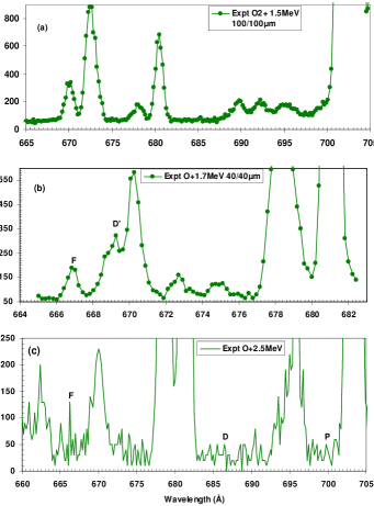
Figure 2: Beam-foil spectra of oxygen. Beam energies and spectrometer slit widths are indicated. Units of intensities are arbitrary. F, D and P: 1s2s2p²3d ⁶L_J-1s2p³3d ⁶D${}_{J^{\prime}}^{o}$, L=F, D and P transitions in O IV. D’: 1s2s2p²3p ⁶D${}_{J}^{o}$-1s2p³3p ⁶P${}_{J^{\prime}}$ transition in O IV Lin and berry  et al (2003).

Fig. 2(a) -2(c) display three typical spectra of oxygen at beam energies of 1.5, 1.7 and 2.5 MeV in the wavelength range of 660-710 Å. In the wavelength region of 660-710 Å transitions between the sextet states 1s2s2p²3d ⁶L - 1s2p³3d ⁶D, L=F, D, P in O IV were expected. At an O₂⁺ beam energy of 1.5 MeV, O₂⁺ ions are mainly excited to terms of O²⁺ and O³⁺. There are no lines emitted from sextet states in O IV in Fig. 2(a). At an O⁺ beam energy of 1.7 MeV, O⁺ ions are mainly excited to terms of O³⁺ and O⁴⁺. New and unidentified emissions appear in the spectrum in Fig. 2(b). Fig. 2(c) shows a spectrum with better resolution to see details of lines.

For the 1s2s2p²3d ⁶L - 1s2p³3d ⁶D, L=F, D, P transitions we expected to resolve fine structures of the lower states 1s2s2p²3d ⁶L in the experiments, whereas fine structures of the upper states 1s2p³3d ⁶D are close and less than resolution of the experimental spectra. O V 3p-4d, O IV 2s²3p-2s²5s, O V 2s3d-2s4f and O III 2s²2p²-2s2p³ transitions are at 659.589 Å, 670.601 Å, 681.332 Å and 703.854 Å, respectively, close to the neighborhood of the doubly excited sextet transitions. The four wavelengths have been semiempirically fitted with high accuracy $\pm$0.004 Å by  Bockasten and Johansson (1968); Pettersson (1982); Moore (1965-1983) and provide a good calibration for the measurements. Standard error for wavelength calibration is $\pm$0.01 Å in the wavelength region of 660-710 Å. Nonlinear least square fits of Gaussian profiles gave values for wavelengths, intensities and full widths at half maximum (FWHM) of lines. Uncertainties of wavelengths are related to intensities of lines. Through the use of optical refocusing we achieved spectroscopic line width of 0.3 Å. Precision of the profile-fitting program was checked through several known transition wavelengths.

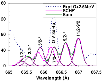
Figure 3: Relative intensity of the 1s2s2p²3d ⁶F_J - 1s2p³3d ⁶D${}^{o}_{J^{\prime}}$ transition in O IV in the experimental spectrum of oxygen at a beam energy of 2.5 MeV. Unit of intensity is arbitrary. * represents all possible J’s of the upper state allowed by E1 transition rules.

Most of new identifications have been obtained by searching in the spectra for sets of unidentified lines and by comparing energies and relative intensities of the 1s2s2p²3d ⁶L-1s2p³3d ⁶D^o, L=F, D and P transitions with results of calculations by MCHF and MCDF approaches. A promising candidate for the 1s2s2p²3d ⁶F_11/2-1s2p³3d ⁶D${}_{9/2}^{o}$ transition appears at the wavelength of 666.99$\pm$0.06 Å in the spectra in Fig. 2(b) and 2(c) recorded at ²⁰O⁺ ion beam energies of 1.7 and 2.5 MeV, which does not appear in the spectrum in Fig. 2(a) recorded at ²⁰O${}_{2}^{+}$ ion beam energy of 1.2 MeV. Shown in Fig. 3 are details of the 1s2s2p²3d ⁶F^o-1s2p³3d ⁶D transition in O IV recorded at an O⁺ ion energy of 2.5 MeV. The curve SCHF’ is convoluted theoretical profile of fine structure components with a Gaussian function. The experimental width of 0.3 Å for the oxygen spectrum was utilized. The transition rates to fine structure j=11/2 to 1/2 of the lower state were results of single-configuration Hartree-Fock (SCHF) calculations by this work. The wavelengths of fine structure components were calculated SCHF results plus a fitted shift for all five components. Measured wavelength of a component is the weighted center of the fitted profile of experimental data. Experimental transition rate is proportional to area of a peak (fitted intensity$\times$FWHM of experimental data). The curve ”Sum” is summation of fitted fine structure components of experimental data. Ratio of measured transition rates for J=11/2-9/2, 9/2-*, J=7/2-*, J=5/2-*, J=3/2-* and J=1/2-* components at an ion energy of 2.5 MeV in Fig. 3 is about 67.4$\times$0.3:56.3$\times$0.3:45.5$\times$0.3:46.2$\times$0.28:20.9$\times$0.3:11.3$\times$0.3 = 5.96:4.98:4.02:3.81:1.85:1.00. * represents all possible j’s of the upper state 1s2p³3p ⁶P_j allowed by electric-dipole transition rules. The ratio is slightly different from theoretical ratio of E1 GF values (in length gauge) of SCHF calculations of 1.188:0.990:0.793:0.595:0.397:0.198 = 6.00:5.00:4.00:3.00:2.00:1.00. Based on above analysis we assign the set of lines as the 1s2s2p²3d ⁶F-1s2p³3d ⁶D^o transition in O IV, and determine their wavelengths with good accuracy of $\pm$0.06 Å.

Table 1: Energies E (in cm-1) and wavelengths $\lambda$ (in Å) for the 1s2s2p²3d ⁶L_J - 1s2p³3d ⁶D${}_{J^{\prime}}$, L= F, D, P transitions in O IV by this work. We list differences dE between theoretical and experimental transition energies for the transitions.

J-J’	$\lambda$exp	Eexp	$\lambda$mchf	Emchf	dEmchf	$\lambda$schf	Eschf	dEschf	$\lambda$mcdf	Emcdf	dEmcdf	$\lambda$scdf	Escdf	dEscdf
	$\pm$0.06
1s2s2p23d 6FJ - 1s2p33d 6D${}_{J^{\prime}}$
				$\pm 106$			$\pm 167$			$\pm 385$			$\pm 783$
1/2-*	665.38	150290	665.83	150188	-102	666.07	150134	-156	663.74	150661	371	661.98	151062	772
3/2-*	665.65	150229	666.08	150132	-97	666.25	150094	-135	663.93	150618	389	662.18	151016	787
5/2-*	665.92	150168	666.32	150078	-90	666.56	150024	-144	664.25	150546	378	662.49	150946	777
7/2-*	666.27	150089	666.69	149995	-95	666.74	149984	-106	664.65	150455	366	662.88	150857	768
9/2-*	666.63	150008	667.10	149903	-106	667.35	149846	-162	665.08	150358	350	663.31	150759	751
11/-9/2	666.99	149927	667.47	149819	-108	667.73	149761	-166	665.51	150261	333	663.72	150666	739
AV	666.41	150058	666.86	149957	-101	667.06	149911	-147	664.83	150415	357	663.06	150817	759
QED				-23.2			-23.2
HO				270.8			84.6
AVT			665.76	150205	147	666.79	149972	-86
nonrel						670.72	149094	-964
1s2s2p23d 6DJ - 1s2p33d 6D${}_{J^{\prime}}$
				$\pm 106$			$\pm 167$			$\pm 385$			$\pm 783$
1/2-*	686.42	145683	685.35	145911	227	688.18	145311	-373	684.20	146156	473	682.24	146576	893
3/2-*	686.39	145690	685.32	145917	227	688.15	145317	-373	684.18	146160	471	682.22	146580	891
5/2-*	686.39	145690	685.30	145921	232	688.15	145317	-373	684.47	146098	409	682.23	146578	888
7/2-*	686.51	145664	685.41	145898	234	688.27	145292	-372	684.27	146141	477	682.35	146552	888
9/2-7/2	686.87	145588	685.76	145824	236	688.63	145216	-372	684.71	146047	459	682.73	146471	883
AV	686.58	145649	685.49	145881	233	688.34	145276	-372	684.44	146105	456	682.43	146536	887
QED				-23.1			-23.0
HO				93.1			209.8
AVT			685.15	145951	302	687.46	145463	-186
N-REL						692.20	144467	-1182
1s2s2p23d 6PJ - 1s2p33d 6D${}_{J^{\prime}}$
				$\pm 869$			$\pm 650$			$\pm 1705$			$\pm 590$
3/2-*	698.06	143254	693.88	144117	863	701.21	142611	-644	689.94	144940	1686	695.23	143837	583
5/2-*	698.57	143150	694.42	144005	855	701.76	142499	-651	690.42	144839	1690	695.76	143728	578
7/2-*	698.95	143072	694.73	143941	869	702.08	142434	-638	690.71	144779	1707	696.08	143662	590
AV	698.63	143138	694.25	144041	902	701.59	142534	-604	690.27	144871	1732	695.60	143762	624
QED				-23.0			-22.9
HO				282.0			112.1
AVT			693.00	144300	1162	701.11	142623	-515
N-REL						705.59	141725	-1413

Similarly, after studying details of transitions theoretically and experimentally described above, and comparing with multi-configuration Hartree-Fock (MCHF) and multi-configuration Dirac-Fock (MCDF) calculations of O IV by this work, we were able to assign these unidentified observed lines as the 1s2s2p²3d ⁶L-1s2p³3d ⁶D^o, L=F, D and P electric-dipole transitions in O IV. Results of the identification and measurements of wavelengths of the transitions are listed in Table I. Errors of measured wavelengths of $\pm$0.06 Å are small mainly from calibration and curve fitting. The latter includes experimental and statistical errors. In Table I average theoretical transition energy AV is the center of gravity of the 1s2s2p²3d ⁶L-1s2p³3d ⁶D^o transition energies (computed from fine structure lines calculated by this work) with results of theoretical analysis. Experimental transition energy AV is the center of gravity of the 1s2s2p²3d ⁶L-1s2p³3d ⁶D^o transition energies (computed from observed lines) with results of experimental transition rate analysis. AV^T is summation of above average transition energy (AV), QED effect (QED) and higher-order correction (HO). Errors for calculated transition energies in Table I are the root mean squared differences of calculated and experimental transition energies as given below in the table. We also list calculated non-relativistic transition energies (N-REL) by SCHF method. In Table I we present measured fine structure wavelength values and theoretical values for O IV. The measured and calculated results are consistent after considering experimental and theoretical errors. Fourteen lines are new observations with wavelength accuracy of $\pm$0.06 Å.

Table 2: Wavelengths $\lambda$ (in Å) for the 1s²2p3p ¹D₂-1s²2p4d ¹F₃ transitions in O V.

$\lambda obs^{a}$	$\lambda obs^{b}$	$\lambda scdf^{a}$	$\lambda schf^{a}$
$\pm 0.06$	$\pm 0.03$
666.27	666.819	651.12
599.85			589.09

a this work. b Elden Moore (1965-1983).

It is noted that in Fig. 2 the line for the 1s2s2p²3d ⁶F_7/2-1s2p³3d ⁶D${}_{J^{\prime=\ast}}^{o}$ transition in O IV is much stronger than the SCHF result. The line is a blend of the 1s2s2p²3d ⁶F_J=7/2-1s2p³3d ⁶D${}_{J^{\prime=\ast}}^{o}$ transition in O IV and a line at the wavelength of 666.27$\pm$0.06 Å. The latter was identified as the 1s²2p3p ¹D₂-1s²2p4d ¹F₃ transition at the wavelength of 666.819$\pm$0.03 Å Bockasten and Johansson (1968); Pettersson (1982); Moore (1965-1983). In this work we could resolve the set of lines and improve the wavelength accuracy of the 1s²2p3p ¹D₂-1s²2p4d ¹F₃ transition to 666.27$\pm$0.06 Å. We list results in Table II. For the 1s²2p3p ¹D₂ state there are two couplings, 1s²2p(j=1/2)3p(j’=3/2) ¹D₂ and 1s²2p(j=3/2)3p(j’=1/2) ¹D₂. For the 1s²2p4d ¹F₃ state there are two couplings, 1s²2p(j=1/2)4d(j’=5/2) ¹F₃ and 1s²2p(j=3/2)4d(j’=3/2) ¹F₃. Their energies are different. MCHF and MCDF methods handle it in different ways and give different results. MCHF calculation gives the minimum energies among both configurations. In Table II are listed wavelengths of SCHF and SCDF calculations. We studied the spectrum in the wavelength range around 590 Å and found a strong unidentified line located at 599.85$\pm$0.06 Å. After studying its details, we assign it as the 1s²2p3p ¹D₂-1s²2p4d ¹F₃ transition in O V and list it in Table II.

Table 3: Energies E (in cm-1) and wavelengths $\lambda$ (in Å) for the 1s2s2p²3d ⁶L_J-1s2p³3d ⁶D_J′, L= F, D, P transitions in F V by this work. We list differences dE between theoretical and experimental transition energies for the transitions.

J-J’	$\lambda$exp	Eexp	$\lambda$mchf	Emchf	dEmchf	$\lambda$schf	Eschf	dEschf	$\lambda$mcdf	Emcdf	dEmcdf	$\lambda$scdf	Escdf	dEscdf
	$\pm$0.10
1s2s2p23d 6FJ - 1s2p33d 6D${}_{J^{\prime}}$
				$\pm 249$			$\pm 156$			$\pm 596$			$\pm 1041$
1/2-*	571.76	174899	571.40	175009	110	572.27	174743	-156	569.83	175491	592	568.94	175765	867
3/2-*	572.01	174822	571.64	174935	113	572.52	174666	-156	570.07	175417	595	568.17	176004	1182
5/2-*	572.41	174700	572.05	174810	110	572.92	174544	-156	570.48	175291	591	569.59	175565	865
7/2-*	572.91	174547	572.55	174657	110	573.42	174392	-155	571.02	175125	578	570.13	175399	851
9/2-*	573.48	174374	572.58	174648	274	573.99	174219	-155	571.62	174941	567	570.75	175208	834
11/2-9/2	574.05	174201	573.15	174474	274	574.56	174046	-155	572.23	174755	554	571.37	175018	817
AV	573.16	174471	572.52	174668	196	573.67	174316	-155	571.28	175044	573	570.31	175343	871
QED				-41.1			-41.1
HO				104.0			121.1
AVT			572.31	174731	260	573.41	174396	-75
N-REL						578.11	172977	-1494
1s2s2p23d 6DJ - 1s2p33d 6D${}_{J^{\prime}}$
				$\pm$104			$\pm$564			$\pm$549			$\pm$830
1/2-*	591.85	168962	591.51	169059	97	593.83	168398	-563	589.97	169500	538	588.97	169788	826
3/2-*	591.82	168970	591.48	169067	97	593.80	168407	-563	589.93	169512	541	588.94	169797	826
5/2-*	591.86	168959	591.51	169059	100	593.84	168396	-563	589.96	169503	544	588.98	169785	826
7/2-*	592.05	168905	591.69	169007	103	594.03	168342	-563	590.14	169451	547	589.18	169727	823
9/2-*	592.52	168771	592.15	168876	105	594.50	168209	-562	590.70	169291	520	589.70	169578	807
AV	592.12	168883	591.77	168985	102	594.10	168321	-563	590.25	169419	536	589.27	169702	819
QED				-40.8			-40.8
HO				249.7			63.4
AVT			591.04	169194	311	594.02	168344	-539
N-REL						598.88	166978	-1905
1s2s2p23d 6PJ - 1s2p33d 6D${}_{J^{\prime}}$
				$\pm$353			$\pm$1861			$\pm$1235			$\pm$475
3/2-*	604.10	165536	603.27	165763	228	610.97	163674	-1861	599.75	166736	1201	605.84	165060	-475
5/2-*	604.88	165322	603.99	165566	244	611.75	163465	-1857	600.45	166542	1220	606.60	164853	-469
7/2-*	605.36	165191	604.03	165555	364	612.22	163340	-1851	600.87	166425	1234	607.08	164723	-468
AV	604.64	165388	603.68	165651	263	611.51	163530	-1857	600.23	166602	1215	606.37	164916	-472
QED				-40.6			-40.5
HO				53.0			175.8
AVT			603.63	165663	275	611.00	163665	-1723
N-REL						616.56	162190	-3197

We obtained spectra at a ²⁰(HF)⁺ beam energy of 2.5 MeV for fluorine. Through the use of optical refocusing we achieved spectroscopic line width of 0.7 Å. Using similar experimental analysis as described above we obtained the wavelength accuracy of $\pm$0.10 Å for the 1s2s2p²3d ⁶L-1s2p³3d ⁶D transitions in the wavelength region of 570-620 Å Moore (1949); Engström (1985). In Table III all observed lines for the 1s2s2p²3d ⁶L - 1s2p³3d ⁶D^o , L=F, D, P transitions in F V are reported. Fourteen lines are new observations. The strongest fine structure component is the 1s2s2p²3d ⁶F_11/2-1s2p³3d ⁶D${}_{9/2}^{o}$ transition at the wavelength of 574.05$\pm$0.10 Å.

Table 4: Energies E (in cm-1) and wavelengths $\lambda$ (in Å) for the 1s2s2p²3d ⁶L_J-1s2p³3d ⁶D${}_{J\prime}^{o}$, L= F, D, P transitions in Ne VI by this work. We list differences dE between theoretical and experimental transition energies for the transitions.

J-J’	$\lambda$exp	Eexp	$\lambda$mchf	Emchf	dEmchf	$\lambda$schf	Eschf	dEschf	$\lambda$mcdf	Emcdf	dEmcdf	$\lambda$scdf	Escdf	dEscdf
	$\pm$0.05
1s2s2p23d 6FJ - 1s2p33d 6D${}_{J^{\prime}}$
				$\pm$3448			$\pm$180			$\pm$811			$\pm$946
1/2-*	500.40	199840	492.42	203079	3239	500.79	199684	-156	498.37	200654	814	498.03	200791	951
3/2-*	500.66	199736	492.69	202967	3231	501.12	199553	-183	498.67	200533	797	498.35	200662	926
5/2-*	501.18	199529	493.12	202790	3261	501.62	199354	-175	499.18	200329	799	498.86	200457	928
7/2-*	501.84	199267	493.69	202556	3290	502.27	199096	-171	499.88	200048	781	499.54	200184	917
9/2-*	502.71	198922	494.26	202323	3401	503.03	198795	-127	500.69	199724	803	500.33	199868	946
11/2-9/2	503.45	198629	496.86	201264	2634	503.80	198491	-138	501.53	199390	760	501.17	199533	904
AV	502.23	199111	494.49	202227	3116	502.62	198959	-152	500.26	199897	786	499.91	200035	924
QED				-67.2			-67.1
HO				94.1			-2.3
AVT			494.43	202254	3143	502.79	198890	-221
N-REL						508.95	196483	-2628
1s2s2p23d 6DJ - 1s2p33d 6D${}_{J^{\prime}}$
				$\pm$2509			$\pm$671			$\pm$745			$\pm$891
1/2-*	519.65	192437	513.56	194719	2282	521.42	191784	-653	517.81	193121	684	517.41	193270	833
3/2-*	519.63	192445	513.55	194723	2278	521.41	191788	-657	517.78	193132	688	517.40	193274	829
5/2-*	519.70	192419	513.49	194746	2327	521.49	191758	-660	517.83	193114	695	517.48	193244	825
7/2-*	520.14	192256	513.57	194715	2459	521.75	191663	-593	518.10	193013	757	517.74	193147	891
9/2-*	520.81	192009	513.94	194575	2567	522.33	191450	-559	518.82	192745	736	518.39	192905	896
AV	520.17	192243	513.67	194676	2433	521.82	191635	-608	518.22	192967	724	517.84	193111	868
QED				-66.7			-66.6
HO				-16.5			-85.3
AVT			513.89	194593	2350	522.24	191483	-760
N-REL						527.59	189541	-2702
1s2s2p23d 6PJ - 1s2p33d 6D${}_{J^{\prime}}$
				$\pm$8011			$\pm$1274			$\pm$2526			$\pm$273
3/2-*	537.00	186220	517.23	193338	7118	540.69	184949	-1271	530.01	188676	2456	536.33	186452	233
5/2-*	538.10	185839	518.34	192924	7085	541.74	184590	-1249	530.92	188352	2513	537.32	186109	270
7/2-*	538.69	185636	529.08	189007	3372	542.39	184369	-1266	531.50	188147	2511	537.94	185894	259
AV	537.74	185963	520.23	192221	6259	541.42	184700	-1262	530.64	188450	2487	537.02	186214	251
QED				-66.4			-66.2
HO				-100.4			-219.8
AVT			520.69	192054	6091	542.26	184414	-1549
N-REL						547.62	182608	-3354

We obtained spectra at a ²⁰Ne⁺ ion beam energy of 4.0 MeV for neon. Through the use of optical refocusing we achieved spectroscopic line width of 0.4 Å in the second order spectrum. Similarly, we obtained wavelength accuracy of $\pm$0.05 Å for the 1s2s2p²3d ⁶L - 1s2p³3d ⁶D^o transitions in the wavelength region of 490-550 Å Brown (1969); Vainshtein and Safronova (1985). In Table IV we present measured fine structure wavelength values and theoretical values for the 1s2s2p²3d ⁶L_J-1s2p³3d ⁶D${}_{J\prime}^{o}$, L=F, D, P transitions for Ne VI. Fourteen lines are new observations. The strongest fine structure component is the 1s2s2p²3d ⁶F_11/2-1s2p³3d ⁶D${}_{9/2}^{o}$ transition at the wavelength of 503.45$\pm$0.05 Å.

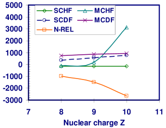
Figure 4: Difference (in cm^-1) between theoretical and experimental transition energies for the 1s2s2p²3d ⁶F - 1s2p³3d ⁶D^o transitions.

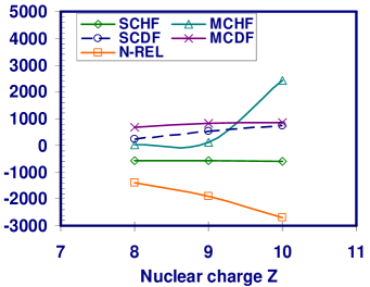
Figure 5: Difference (in cm^-1) between theoretical and experimental transition energies for the 1s2s2p²3d ⁶D - 1s2p³3d ⁶D^o transitions.

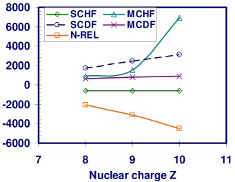
Figure 6: Difference (in cm^-1) between theoretical and experimental transition energies for the 1s2s2p²3d ⁶P - 1s2p³3d ⁶D^o transitions.

We have studied differences between experimental and theoretical transition energies of the 1s2s2p²3d ⁶L - 1s2p³3d ⁶D^o transitions along B I isoelectronic sequence. In Fig. 4, 5 and 6 are plots of differences between theoretical and experimental transition energies of the 1s2s2p²3d ⁶L - 1s2p³3d ⁶D^o, L=F, D, P transitions in boron-like ions. Here theoretical transition energy is the center of gravity of the 1s2s2p²3d ⁶L_J-1s2p³3d ⁶D${}_{J\prime}^{o}$ transition energies (computed from calculated fine structure lines by this work) with results of theoretical analysis, and experimental transition energy is the center of gravity of the 1s2s2p²3d ⁶L_J-1s2p³3d ⁶D${}_{J\prime}^{o}$ transition energies (computed from observed lines) with results of experimental analysis. In Fig. 4 MCDF, SCHF and SCDF differences are constant for the 1s2s2p²3d ⁶F - 1s2p³3d ⁶D^o transitions with nuclear charge Z = 8, 9 and 10. Non-relativistic differences (N-REL) are linear. MCHF differences for oxygen and fluorine are small, just 106 and 249 cm^-1.

In Fig. 5 SCHF, SCDF and MCDF differences are constant for the 1s2s2p²3d ⁶D - 1s2p³3d ⁶D^o transitions with nuclear charge Z = 8, 9 and 10. Non-relativistic differences are linear. MCHF differences for oxygen and fluorine are small, just 235 and 104 cm^-1.

In Fig. 6 SCHF and MCDF differences are constant for the 1s2s2p²3d ⁶P - 1s2p³3d ⁶D^o transitions with nuclear charge Z = 8, 9 and 10. SCDF and non-relativistic differences are linear. These linear or constant energy differences can be used to predict easily and with high accuracy transition energies for the 1s2s2p²3d ⁶L - 1s2p³3d ⁶D^o, L=F, D, P transitions for boron-like ions with 5$<$Z$<$13.

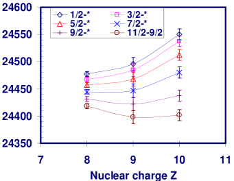
Figure 7: Reduced experimental transition energies E/(Z-1.86) (in cm^-1) for the 1s2s2p²3d ⁶F_J-1s2p³3d ⁶D${}_{J\prime}^{o}$ transitions.

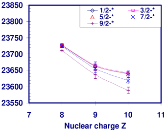
Figure 8: Reduced experimental transition energies E/(Z-1.86) (in cm^-1) for the 1s2s2p²3d ⁶D_J-1s2p³3d ⁶D${}_{J\prime}^{o}$ transitions.

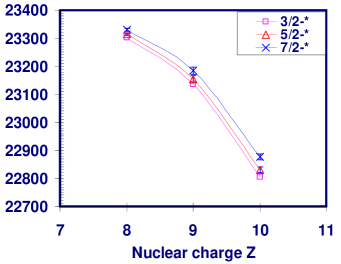
Figure 9: Reduced experimental transition energies E/(Z-1.86) (in cm^-1) for the 1s2s2p²3d ⁶P_J-1s2p³3d ⁶D${}_{J\prime}^{o}$ transitions.

In Fig. 7, 8 and 9 are summarized details of experimental fine structures of the 1s2s2p²3d ⁶L_J, L=F, D, P states in O IV, F V and Ne VI. Comparisons of measured fine structures of the 1s2s2p²3d ⁶L_J states show reasonable tendency. Here error bars are from experiments.

Table 5: Lifetimes (in ps) of the 1s2s2p²3d ⁶P and 1s2p³3d ⁶D^o states in N III, O IV, F V, Ne VI and Na VII.

Ion	This work			others
	MCHF	SCHF	MCDF	Expt	Theory
1s2s2p23d 6P
N III	45.37	40.65	47.42	66$\pm$12a	42.8$\pm$18b
O IV	15.32	15.29	16.01	12$\pm$3a	14.95$\pm$4b
F V	6.82	6.90	7.02	11$\pm$4a	6.689$\pm$4b
Ne VI	3.57	3.54	3.61
Na VII	2.10	2.04	2.07
1s2p33d 6Do
N III	275.3	286.2	255.3
O IV	225.7	238.7	213.1
F V	196.7	204.3	183.3
Ne VI	170.1	178.1	153.0
Na VII	150.8	157.4	140.0

a Blanke  Blanke et al (1992). b Miecznik  Miecznik  et al (2000).

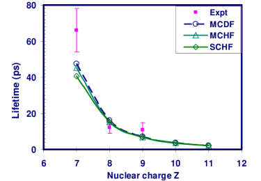
Figure 10: Lifetimes (in ps) for the 1s2s2p²3d ⁶P^e states in B I isoelectronic sequence. Experimental values are taken from Table V.

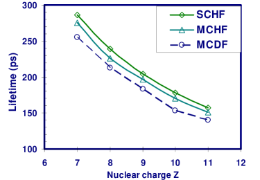
Figure 11: Lifetimes (in ps) for the 1s2p³3d ⁶D^o states in the boron sequence.

MCHF, SCHF and MCDF calculated lifetimes for the 1s2s2p²3d ⁶P and 1s2p³3d ⁶D^o states in N III, O IV, F V Ne VI and Na VII by this work are listed in Table V, and compared with results of measurements of Blanke et al  Blanke et al (1992) and calculations of Miecznik et al Miecznik  et al (2000). They are plotted in Fig. 10 and 11. Discrepancy between theory and experiments is around or larger than experimental errors (see Fig. 10), most probably due to additional decay modes of M2 and radiative autoionization or some missing configurations which are important for MCHF and MCDF calculations.

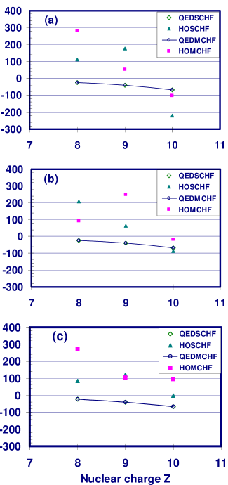
Figure 12: QED and higher-order corrections (in cm^-1) for (a) the 1s2s2p²3d ⁶F - 1s2p³3d ⁶D^o, (b) 1s2s2p²3d ${}^{6}D$ - 1s2p³3d ⁶D^o and (c) 1s2s2p²3d ⁶P - 1s2p³3d ⁶D^o transitions in B I isoelectronic sequence.

QED and higher-order corrections for the 1s2s2p²3d ⁶L - 1s2p³3d ⁶D${}^{o},$ L=F, D, P transitions in O IV, F V and Ne VI are up to -220-370 cm-1 (see Table I, III and IV) and can’t be ignored in careful comparison with experiments. Here QED and higher-order corrections were calculated from effective nuclear charge Z_eff obtained from MCHF and SCHF calculations. In Fig. 11 are plots of the above corrections to weighted mean transition energies. The results show that weighted mean wavelengths for the 1s2s2p²3d ⁶L - 1s2p³3d ⁶D${}^{o},$ L=F, D, P transitions in O IV, F V and Ne VI are sensitive to QED and higher-order corrections to 0.27 Å, 0.26 Å and 0.18 Å, respectively. They are larger than estimated experimental precision of $\pm$0.06 Å, $\pm$0.10 Å and $\pm$0.05 Å. Transition energies are strongly related to electron correlation. We could not get exact electron correlation. QED and higher-order corrections of sextet states in boron-like systems are large enough to be seen experimentally. This work could provide a good test for QED and higher-order corrections if electron correlation were known.

V CONCLUSIONS

We performed MCHF (with QED and higher-order corrections) and MCDF calculations to get energies, lifetimes and relevant E1 transition wavelengths and rates for the 1s2s2p²3d ⁶L - 1s2p³3d ⁶D^o , L=F, D, P electric-dipole transitions in five-electron O IV, F V and Ne VI. Present beam-foil study of oxygen, fluorine and neon led to observations of 42 new lines in the sextet system of O IV, F V and Ne VI. We measured wavelengths with good accuracy. Identifications are mainly obtained by comparing transition wavelengths and rates with results of MCHF and MCDF calculations. Theoretical and experimental transition energies are consistent in errors. Differences between theoretical and experimental transition energies are in reasonable range. For lifetimes of the 1s2s2p²3d ⁶P states in O IV and F V there remain large discrepancies of about 20% between results of MCHF and MCDF calculations and experiments from Blanke et al (1992).

References

- Blanke et al (1992) J. H. Blanke, B. Fricke, P. H. Heckmann and E. Träbert, Phys. Scr. 45, 430 (1992).
- Lapierre and Knystautas (2000) L. Lapierre and E. J. Knystautas, J. Phys. B 33, 2245 (2000).
- Lin and berry et al (2003) Bin Lin, H. Gordon Berry, and Tomohiro Shibata, A. E. Livingston, Henri-Pierre Garnir, Thierry Bastin, J. Désesquelles, Igor Savukov, Phys. Rev. A 67, 062507 (2003).
- Berry et al (1975) H. G. Berry, T. Bastin, E. Biemont, P. D. Dumont and H. P. Garnir, Rep. Prog. Phys. 5, 12 (1975).
- Kramida et al (1999) A. E. Kramida, T. Bastin, E. Biemont, P. D. Dumont and H. P. Garnir, J. Opt. Soc. Am. B 16 (11), 1966 (1999).
- Miecznik et al (2000) G. Miecznik, T. Brage and C. F. Fischer, Phys. Scr. 45, 436 (1992).
- Fischer et al (2000) C. F. Fischer, T. Brage and P. Jonsson, Computational Atomic Structure an MCHF Approach (Institute of Physics Publishing, Bristal and Philadelphia (1997).
- Chung et al (1992) K. T. Chung, X. W. Zhu and Z. W. Wang, Phys. Rev. A 29, 682 (1984).
- Dyall & Grant et al (1989) K. G. Dyall, and I. P. Grant, computer physics communications 55, 425 (1989).
- Parpia, Fischer and Grant (1996) F. A. Parpia, C. F. Fischer, and I. P. Grant, Computer Physics Communications 94 (2-3), 249 (1996).
- Fritzsche and Grant & Grant et al (1997) S. Fritzsche, and I. P. Grant, Computer Physics Communications 103 (2-3), 277 (1997).
- Chung et al (1992) K. T. Chung, X. W. Zhu and Z. W. Wang, Phys. Rev. A 47 (3) 1740 (1992).
- Chung et al (1993) K. T. Chung and X. W. Zhu, Phys. Rev. A 48(3) 1944 (1993).
- Drake and Swainson (1990) G. W. F. Drake and R. A. Swainson, Phys. Rev. A 41 (3) 1243 (1990),
- Berry et al (1982) H. G. Berry, R. L. Brooks, K. T Cheng, J. E. Hardis and W. Ray, Phys. Scr. 42, 391 (1982).
- Hardis et al (1984) J. E. Hardis, H. G. Berry, L. G. Curtis and A. E Livingston, Phys. Scr. 30, 189 (1984).
- Garnir et al (1988) H. P. Garnir, Y. Baudinet-Robinet, and P. D. Dumont, Nuclear Instruments and Methods in Physics Research B 31, 161 (1988).
- Baudinet-Robinet et al (1990) Y. Baudinet-Robinet, and P. D. Dumont, H. P. Garnir, PhysicaliaMag. 12, 3 (1990).
- Girardeau et al (1971) R. Girardeau and E. J. Knystautas, G. Beauchemin sj B. Neveu R. Drouin J. Phys. B 4, 1743 (1971).
- Lin and berry et al (2003) Bin Lin, H. Gordon Berry, and Tomohiro Shibata, A. E. Livingston, Henri-Pierre Garnir, Thierry Bastin, J. Désesquelles, sumitted to Phys. Rev. A , (2004). eprint arXiv:physics/0404001.
- Bockasten and Johansson (1968) K. Bockasten and K. B. Johansson, Ark. Fys. 38, 563 (1968).
- Pettersson (1982) S. G. Pettersson, Phys. Scr. 26, 296 (1982).
- Moore (1965-1983) C. E Moore, NSRDS-NBS 3, Section 1-10 (1965-1983).
- Moore (1949) C. E Moore, Atomic Energy Levels 1, Circ. Natl. Bur. Stand. 467 (1949).
- Engström (1985) L. Engström, Phys. Scr. 29, 113 (1985).
- Brown (1969) R. T. Brown, APJ 158, 829 (1969).
- Vainshtein and Safronova (1985) L. A. Vainshtein and U. I. Safronova, Phys. Scr. 31, 519 (1985).