Apparent slip due to the motion of suspended particles in flows of electrolyte solutions

Abstract

We consider pressure-driven flows of electrolyte solutions in small channels or capillaries in which tracer particles are used to probe velocity profiles. Under the assumption that the double layer is thin compared to the channel dimensions, we show that the flow-induced streaming electric field can create an apparent slip velocity for the motion of the particles, even if the flow velocity still satisfies the no-slip boundary condition. In this case, tracking of particle would lead to the wrong conclusion that the no-slip boundary condition is violated. We evaluate the apparent slip length, compare with experiments, and discuss the implications of these results.

1 Introduction

The no-slip boundary condition of fluid mechanics states that the velocity of a viscous flow vanishes near a stationary solid surface [1]. Although it has been a crucial ingredient of our understanding of fluid mechanics for more than a century, it has been much debated in the past [2], and, in the case of liquids, a complete physical picture for its origin has yet to be given. The ongoing debate stems from the fact that it is an assumption which cannot be derived from first principles. It has been shown that on length scales much larger than the scale of surface heterogeneities, the no-slip condition might be a macroscopic consequence of inevitable microscopic roughness [3, 4], but the case of perfectly smooth surfaces has yet to be explained. In particular, the physico-chemical properties of both the fluid and the solid surface certainly are important.

Only a few experimental studies have addressed the no-slip condition in the past [5, 6], and it is only the recent advances in the controlled fabrication of micro- and nano-devices and in the corresponding measurement techniques that have allowed the problem to be reconsidered. Over the last few years, a number of pressure-driven flow [7, 8, 9, 10], shear-flow [11], and squeeze-flow experiments [12, 13, 14, 15, 16, 17, 18] showing a response interpretable as some degree of slip for partially wetting liquids have been reported. Molecular dynamics simulations of Lennard-Jones liquids have also shown that slip can occur, but only at unrealistically high shear rates [19, 20].

Fluid slip is usually quantified by a slip length $\lambda$. Let us consider for simplicity a unidirectional flow past a solid surface. Following Navier [21], the slip length linearly relates the surface slip velocity to the shear rate of the fluid evaluated at the surface

$$u=\lambda\frac{\partial u}{\partial n}\cdot$$ (1)

The slip length can also be interpreted as the fictitious distance below the surface at which the velocity would be equal to zero if extrapolated linearly: the no-slip boundary condition is equivalent to $\lambda=0$ and a no-shear boundary condition is equivalent $\lambda=\infty$.

Consider pressure-driven flow in a two-dimensional channel of height $2h$. If we assume that the boundary condition on the channel walls ($z=\pm h$) is given by (1), the axial velocity profile in the channel is

$$U_{\rm slip}(z)=-\frac{h^{2}}{2\mu}\frac{{\rm d}p}{{\rm d}x}\left[1-\frac{z^{2}}{h^{2}}+\frac{2\lambda}{h}\right],$$ (2)

which is a Poiseuille flow augmented by a finite plug velocity, which augmented flow rate ${Q_{\rm slip}}$ is given in a non-dimensional form by

$$\frac{Q_{\rm slip}}{Q_{\rm no\mbox{\footnotesize-}slip}}=1+\frac{3\lambda}{h}\cdot$$ (3)

Experimentalists have usually addressed the issue of fluid slip in two distinct ways. The first consists in performing indirect measurements, such as pressure-drop versus flow rate or squeezing rate versus resistance, and then use such measurements to infer a slip length. This procedure is indirect in the sense that it assumes that the flow resembles (2) and then equation (3), or an equivalent, is used to determine $\lambda$ [7, 8, 10, 12, 13, 14, 15, 16, 17, 18].

The second way consists in performing direct velocity measurements in the fluid. We are only aware of two such previous works. Pit et al. [11] measured velocities in shear flow of hexadecane over a smooth surface using a technique based on fluorescence recovery after photobleaching (see also [22]). The measurements were performed down to 80 nm from the solid surface and averaged over a few tens of microns. Fluid slip was observed with $\lambda\sim 100$ nm in the case of lyophobic surfaces. Tretheway & Meinhart (2001) [9] used micro-particle image velocimetry (PIV) techniques to measure the velocities of tracer nanoparticles (radius 150 nm) in pressure-driven channel flow of water. Measurements were made down to 450 nm from the solid surface and cross-correlated to increase signal-to-noise ratios. Results consistent with the no-slip condition were obtained in completely wetting conditions, but slip with $\lambda\sim 1$ $\mu$m was obtained when the channel walls were treated to be hydrophobic.

In this paper, we wish to draw attention to some of the possible consequences of this latter type of particle-based measurements. We address theoretically a prototypical pressure-driven flow experiment in small channels in the case where small tracer particles are used to probe the fluid velocity. We show that if electrical effects for both the channel and the particles are properly taken into account, it is possible for the particles to behave as if they were advected by a flow with a finite non-zero slip length, even if the velocity profile in the fluid surrounding the particle does not violate the no-slip condition.

In the following section we summarize some important background electrostatics and hydrodynamics results, derive the formulae in the case of two dimensional channels and introduce the electroviscous effect. In section 3 we present a physical picture for the effect we report, derive the expressions for the apparent slip lengths and give the conditions for the occurrence of such slip. Finally, in section 4 we discuss implications of these results along with estimates of their order of magnitude under typical experimental conditions and compare with experiments.

2 Flow of an electrolyte solution

The physical picture for the effect we wish to introduce relies on the following known facts.

2.1 Surface charge and electrostatics

A solid surface in contact with an electrolyte solution will in general acquire a net charge, due for example to the ionization of surface groups, ion adsorption and/or dissolution. This surface charge is a thermodynamic property of the solid-electrolyte pair and the reader is referred to [23, 29] for detailed presentations of the phenomenon. The equilibrium surface potential is called the zeta potential $\zeta$.

Such surface charges are screened by a diffusive cloud of counter-ions in the solution. At equilibrium, the electrostatic potential $\psi$ in the electrolyte satisfies the Poisson-Boltzmann equation which quantifies the balance between purely electrostatic interactions and diffusion [23],

$$\nabla^{2}\psi=\frac{2en_{0}}{\epsilon\epsilon_{0}}\sinh\left(\frac{e\psi}{k_{B}T}\right),$$ (4)

where we consider here for simplification only the case of monovalent 1:1 ions, e.g. Na⁺ and Cl^- or OH^- and H⁺.

A convenient approximation usually made to solve (4) is the Debye-Hückel approximation [23, 25, 27, 28] of small field strength, $|e\psi|\ll k_{B}T$, in which case the equation simplifies to the linearized Poisson-Boltzmann equation

$$\nabla^{2}\psi=\kappa^{2}\psi,\quad\kappa^{-1}=\left(\frac{\epsilon\epsilon_{0}k_{B}T}{2e^{2}n_{0}}\right)^{1/2},$$ (5)

where $\kappa^{-1}$ is the Debye screening length: it is the typical length scale in the solution over which counter-ions screen the charged solid surface, and beyond which the net charge density is essentially zero.

However, (5) is restricted to low surface potentials, typically 20mV, which is a severe approximation. Let us consider for simplicity the case of a two-dimensional channel of height $2h$ in the $z$-direction and let us instead derive the solution to (4) for any value of the zeta potential at the wall $\zeta_{w}$ but in the limit where the channel dimensions are much larger than the double layers $\kappa h\gg 1$. This limit is appropriate for channel sizes down to $h\approx 5$ $\mu$m in the case of pure water, or even $h\approx 50$ nm in the case of tap water.

Let us define the dimensionless potential $\phi=e\psi/k_{B}T$ and the dimensionless vertical coordinate $\bar{z}=z/h$. In this case, (4) becomes

$$\frac{1}{(\kappa h)^{2}}\frac{{\rm d}^{2}\phi}{{\rm d}\bar{z}^{2}}=\sinh\phi,$$ (6)

with the boundary conditions $\phi(\bar{z}=\pm 1)=\phi_{w}=e\zeta_{w}/k_{B}T$.

Since $1/\kappa h\ll 1$, the solution to equation (6) involves boundary layers near $z=\pm 1$. The outer solution $\phi_{\rm\,out}$ is found by taking the limit $1/\kappa h=0$ in (6) and we find $\phi_{\rm\,out}=0$. The inner solution $\phi_{\rm\,in}$ is valid near the boundaries for $\kappa h(1-|\bar{z}|)={\cal O}(1)$, in which case (6) reduces to the Poisson-Boltzmann equation near an infinite plane, whose solution is [27]

$$\tanh\left(\frac{\phi_{\rm\,in}(\bar{z})}{4}\right)=\tanh\left(\frac{\phi_{w}}{4}\right)e^{-\kappa h(1-|\bar{z}|)}.$$ (7)

Finally, since $\phi_{\rm\,out}=0$, the inner solution (7) is also equal to the composite solution $\phi(\bar{z})$, uniformly valid throughout the channel as $\kappa h\to\infty$, at leading order in $1/\kappa h$. For convenience, equation (7) can be rewritten as

$$\phi(\bar{z})=2\ln\left(\frac{1+t_{w}e^{-\kappa h(1-|\bar{z}|)}}{1-t_{w}e^{-\kappa h(1-|\bar{z}|)}}\right),$$ (8)

where we have defined $t_{w}=\tanh(e\zeta_{w}/4k_{B}T)$.

2.2 Hydrodynamics and electrokinetics

When a pressure-driven flow occurs in the channel, the fluid velocity is unidirectional ${\bf U}=U(z){\bf e}_{x}$, where ${\bf e}_{x}$ is the streamwise direction. In the absence of electrical effects, the fluid velocity is simply Poiseuille’s pressure-driven formula [1], which we will denote $U_{{\rm PD}}$, and is given by

$$U_{\rm PD}(z)=-\frac{h^{2}}{2\mu}\frac{{\rm d}p}{{\rm d}x}\left[1-\frac{z^{2}}{h^{2}}\right]\cdot$$ (9)

Furthermore, if an external, or induced, electric field ${\bf E}_{S}=E_{S}{\bf e}_{x}$ is also applied to the channel, the presence of a net charge density near the solid surface moving in response to the field leads to an additional velocity component known as electroosmotic flow (EOF) [23]. It is directed in the $x$-direction, is given by

$$U_{{\rm EOF}}(z)=\frac{\epsilon\epsilon_{0}E_{S}}{\mu}\Big{[}\psi(z)-\zeta_{w}\Big{]},$$ (10)

and is valid for any value of $\zeta_{w}$.

2.3 Streaming potential and electroviscous effect

As the electrolyte solution flows down a pressure gradient, the cloud of counter-ions is advected by the flow and a streaming current is established. If no short-circuit is present between the two ends of the capillary, accumulation of charge sets up a potential difference along the channel, termed the “streaming potential”. Such potential, or equivalently electric field, opposes the mechanical transfer of charge by creating a reverse conduction current through the bulk solution such that the total net electric current is zero. This induced axial electric field scales with the applied pressure gradient and leads to the creation of an induced electroosmotic back-flow which effectively slows down the fluid motion in the capillary: a smaller flow rate for a given pressure drop is obtained than in the regular Poiseuille case, as if the liquid had a higher shear viscosity than expected. Consequently this effect is usually referred to as the primary “electroviscous effect” [24, 25, 26, 27, 28].

Let us consider the pressure-driven flow in a channel of height $2h$ and width $w\gg h$ of the electrolyte solution with electrostatic potential given by equation (7). We calculate below the value of the steady-state streaming electric field $E_{S}{\bf e}_{x}$ induced by the flow.

Pressure-driven current

First, the pressure-driven motion of the screening cloud of counter-ions near the charged surface leads to an advection-of-charge electric current $I_{S}^{PD}$ given by

$$I_{S}^{\rm PD}=\int_{-h}^{h}w\rho_{e}(z)U_{{\rm PD}}(z){\rm d}z=\frac{2\epsilon\epsilon_{0}whk_{B}T}{\mu e}\left(\frac{{\rm d}p}{{\rm d}x}\right)I_{1},$$ (11)

where we have used the electrostatic equation to relate the net charge density in the liquid to the electrostatic potential, ${\rho_{e}}=-\epsilon\epsilon_{0}\nabla^{2}\psi$ and where $I_{1}$ is given by

$$I_{1}=\phi_{w}-\int_{0}^{1}\phi(\bar{z}){\rm d}\bar{z},$$ (12)

with the same dimensionless notations as in section 2.1. In the limit where $\kappa h\gg 1$, plugging in the solution (7) into (12) leads to

$$I_{1}=\phi_{w}-\frac{2}{\kappa h}\int_{0}^{\kappa h}\ln\left(\frac{1+t_{w}e^{-x}}{1-t_{w}e^{-x}}\right){\rm d}x,$$ (13)

so that

$$I_{S}^{\rm PD}=\frac{2\epsilon\epsilon_{0}wh\zeta_{w}}{\mu}\left(\frac{{\rm d}p}{{\rm d}x}\right)\left[1+{\cal O}\left(\frac{1}{\kappa h}\right)\right].$$ (14)

Electroosmotic current

If an electric field is induced by the flow, the streaming current has a second component $I_{S}^{{\rm EOF}}$, given by the advection of counter-ions by the induced electroosmotic flow

$$I_{S}^{{\rm EOF}}=\int_{-h}^{h}w\rho_{e}(z)U_{\rm EOF}(z){\rm d}z=\frac{2wE_{S}}{h\mu}\left(\frac{\epsilon\epsilon_{0}k_{B}T}{e}\right)^{2}I_{2},$$ (15)

where $I_{2}$ is given by

$$I_{2}=\int_{0}^{1}\left(\frac{{\rm d}\phi}{{\rm d}\bar{z}}\right)^{2}{\rm d}\bar{z}.$$ (16)

In the limit where $\kappa h\gg 1$, the boundary layer solution (7) leads to the leading order expression for $I_{2}$ in powers of $1/\kappa h$,

$$I_{2}=\frac{8\kappa ht_{w}^{2}(1-e^{-2\kappa h})}{(1-t_{w}^{2})(1-t_{w}^{2}e^{-2\kappa h})},$$ (17)

so that

$$I_{S}^{{\rm EOF}}=\frac{16w\kappa E_{S}}{\mu}\left(\frac{\epsilon\epsilon_{0}k_{B}T}{e}\right)^{2}\left(\frac{t_{w}^{2}}{1-t_{w}^{2}}\right)\left[1+{\cal O}\left(\frac{1}{\kappa h}\right)\right]\cdot$$ (18)

Conduction current

Finally, in response to the electric field, a conduction current $I_{C}$ is set up in the bulk of the solution; if we denote by $\sigma$ the ionic conductivity of the electrolyte (assumed to be constant), the conduction current is given by

$$I_{C}=2hw\sigma E_{S}.$$ (19)

Induced electric field

If we investigate the steady-state motion of the electrolyte solution, we require that there be no net electric current

$$I_{S}^{\rm PD}+I_{S}^{{\rm EOF}}+I_{C}=0,$$ (20)

which leads to the formula for the flow-induced streaming electric field

$$E_{s}=-\frac{{\rm d}p}{{\rm d}x}\left(\frac{\epsilon\epsilon_{0}\zeta_{w}}{\sigma\mu}\right)\left[1+\frac{8\kappa}{\sigma\mu h}\left(\frac{\epsilon\epsilon_{0}k_{B}T}{e}\right)^{2}\left(\frac{t_{w}^{2}}{1-t_{w}^{2}}\right)\right]^{-1}+{\cal O}\left(\frac{1}{\kappa h}\right)\cdot$$ (21)

As expected, the induced field $E_{S}$ is proportional to the applied pressure gradient.

Note that within the Debye-Hückel approximation (5), the induced electric field can be calculated exactly for all values of $\kappa h$ [23, 25, 27, 28] and we find

$$E_{S}=\frac{{\rm d}p}{{\rm d}x}\left(\frac{\tanh\kappa h}{\kappa h}-1\right)\left[\frac{\sigma\mu}{\epsilon\epsilon_{0}\zeta_{w}}+\frac{\epsilon\epsilon_{0}\zeta_{w}\kappa}{4h}\left(\frac{\sinh 2\kappa h-2\kappa h}{(\cosh\kappa h)^{2}}\right)\right]^{-1}\cdot$$ (22)

In the limits where $e|\zeta_{w}|/k_{B}T\ll 1$ (i.e. $t_{w}\ll 1$) and $\kappa h\gg 1$, the expressions given by (21) and (22) agree and are given by

$$E_{S}=-\frac{{\rm d}p}{{\rm d}x}\left(\frac{\epsilon\epsilon_{0}\zeta_{w}}{\sigma\mu}\right)\left[1+\frac{(\epsilon\epsilon_{0}\zeta_{w})^{2}\kappa}{2\sigma\mu h}\right]^{-1}\cdot$$ (23)

3 Velocity of a suspended particle and apparent slip

3.1 Physical picture

We now consider an experiment in which the above electric effects are present. We elect to use small tracer particles to probe the velocity profile, including possible fluid slip, as illustrated in Figure 1. For the same reason as for the capillary surfaces, these particles will usually be charged in solution. As they are advected by the fluid motion, they will also feel the influence of the induced streaming electric field: consequently their velocity will not only reproduce that of the fluid but will also include an induced electrophoretic component [23], proportional to their zeta potential and the streaming electric field. If the zeta potential of a particle has a sign opposite to that of the capillary surface, the particle will be slowed down by the electric field. On the contrary, if the particle possesses a potential of the same sign as the capillary surface, its electrophoretic component will be in the streamwise direction; furthermore, if its zeta potential is large enough, the electrophoretic velocity of the particle will be able to overcome the induced electroosmotic back-flow.

It then follows that there is a significant potential implication of the induced electric field: if one were to conduct an experiment in such conditions without considering any important electrical effects, these particles would go faster than the expected Poiseuille pressure-driven profile, leading to the incorrect conclusion that the velocity profile has a non-zero slip velocity at the wall. Thus, even if the flow satisfies the no-slip condition, measurements of particle velocities would lead to non-zero apparent slip lengths. We shall quantify this mechanism in the following sections.

3.2 Particle velocity

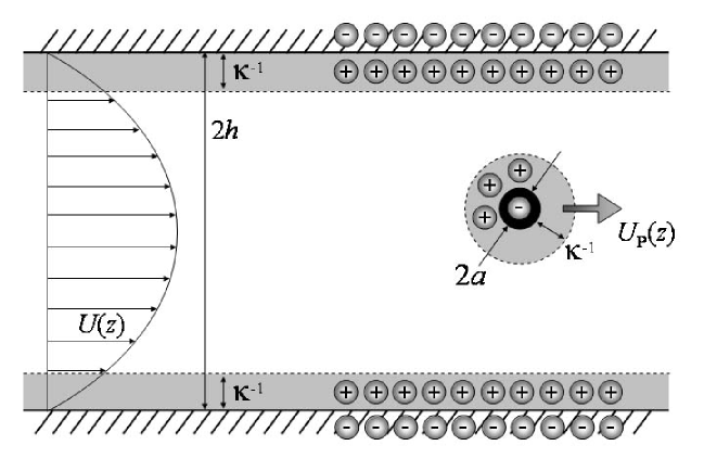
Figure 1: Schematic representation of the flow between two parallel plates with charged surfaces (zeta potential $\zeta_{w}$) and a charged suspended particle (zeta potential $\zeta_{p}$); in the case illustrated, $\zeta_{w}<0$ and $\zeta_{p}<0$. The channel height is $2h$, the particle radius is $a$, the smallest wall-particle distance is $d$ and the screening length $\kappa^{-1}$.

We consider the presence of a single solid spherical particle of radius $a\ll h$ suspended in a two-dimensional channel of height $2h$ where a pressure-driven flow occurs, as illustrated in Figure 1; the particle is located at a distance $d=h-|z|$ from the closest wall. We also assume for simplicity that the presence of the particle does not modify the nature of ionic groups in solution (1:1 monovalent ions), so that the screening lengths $\kappa^{-1}$ for the charged particle and the charged channel surface are the same, as given by equation (5).

The particle velocity ${\bf U}_{\rm P}(z)$ will in general be

$${\bf U}_{\rm P}(z)={\bf U}_{\rm hydro}(z)+{\bf U}_{\rm elec}(z)+{\bf U}_{\rm k_{B}T},$$ (24)

which includes three contributions.

Hydrodynamic contribution

The first component is the hydrodynamic contribution

$${\bf U}_{\rm hydro}(z)=\left[1-{\cal O}\left(\frac{a}{d}\right)\right]U_{\rm PD}(z){\bf e}_{x},$$ (25)

where $U_{\rm PD}$ is the local pressure-driven fluid velocity. It is modified by the presence of solid walls which slow down the motion of the suspended particle. Although the analysis is in general difficult [30], walls lead to a leading-order correction to the particle velocity of order of the ratio of the particle size to the distance to the walls ${\cal O}(a/d)$; this is true as long as the particle does not come too close to the wall, in which case a different contribution arises from lubrication forces. We will assume in this paper that the particle is located sufficiently far from the walls ($a\ll d=h-|z|$) so that the influence of the walls can be neglected. Such a requirement would also have to be verified in an experiment, otherwise the presence of the wall would hinder some component of the measured slip velocity. Note that if walls were not present, a correction to the velocity accounting for the finite size of the particle and the spatial variations of the fluid velocity would also be present, but only at second order in the ratio of the particle size to the length scale over which flow variations occur [31].

Electrical contribution

In general the particle will be charged, with a zeta potential $\zeta_{p}$ which we assume to be uniform. Consequently, its velocity will include a contribution from electrical forces, ${\bf U}_{\rm elec}(z)$. This velocity has two components

$${\bf U}_{\rm elec}(z)={\bf U_{\rm EPH}}+U_{\rm drift}(z)\,{\bf e}_{z},$$ (26)

where ${\bf U_{\rm EPH}}$ is an electrophoretic velocity due to the presence of an external electric field and $U_{\rm drift}(z)$ is a vertical drift due to the electrostatic interactions between the charged particle and the charged walls. Such drift will only be significant if the double layers around the particle and along the channel walls overlap, and will be exponentially screened otherwise [23]. We will assume that such requirement is met in practice $\kappa d\gtrsim{\cal O}(1)$, so that it can be neglected.

When the electric field ${\bf E}_{S}=E_{S}{\bf e}_{x}$ is aligned with the channel direction, the electrophoretic velocity ${\bf U}_{\rm EPH}=U_{\rm EPH}\,{\bf e}_{x}$ is given by

$$U_{\rm EPH}=\frac{\epsilon\epsilon_{0}E_{S}(f(\kappa a)\zeta_{p}-\zeta_{w})}{\mu}\left[1-{\cal O}\left(\frac{a^{3}}{d^{3}}\right)\right]\cdot$$ (27)

This velocity first includes the “pure” electrophoretic mobility of the particle [23, 27, 32], characterized by the function $f(x)$, which satisfies $f(0)=2/3$ (Hückel’s result for thick screening length) and $f(\infty)=1$ (Smoluchowski’s result for thin screening length). Note that we can use these classical electrophoretic formulae because since $\kappa h\gg 1$, the perturbation of the ion distribution in the double layer around the particle is not modified by the local shear flow. The velocity (27) also includes the electroosmotic back-flow resulting from the motion of excess charges near the channel walls and proportional to the wall zeta potential $\zeta_{w}$. Furthermore, the presence of a wall always influences the electrophoretic mobility at cubic order in the ratio of the particle size to the distance to the wall, as long as double layers do not overlap [34, 35]; since we already assumed the particle to be located far from the wall, we will neglect the wall influence here as well.

Thermal contribution

Finally, the particle velocity has a random contribution ${\bf U}_{\rm k_{B}T}$ due to thermal motion, which can be significant. A solid spherical particle of radius $a$, located far from boundaries, has a diffusivity $D$ given by the Stokes-Einstein relation $D=k_{B}T/6\pi\mu a$ [23], corresponding to a root mean square velocity on the order of $U_{k_{B}T}\sim D/a\sim k_{B}T/6\pi\mu a^{2}$. At 25^∘C in water, $a=10$ nm leads to $U_{k_{B}T}\sim 1$ mm/s; this value is of the same order as the fluid velocity in a circular capillary of radius $R\sim 100$ $\mu$m and flow rate $Q\sim 1$ $\mu$L/min, typical values for microfluidic devices. Consequently, we cannot assume that the Peclet number, $Pe=U/U_{k_{B}T}=Ua/D$, is necessarily large and thermal motion cannot in general be neglected. However, in the experiments reported to date, velocity measurements are cross correlated (as in [9]) or averaged (as in [11]) so that the random thermal motion disappears, and we will therefore not consider it in this paper.

Summary

Under the previous assumptions, we can write the velocity for the particle as

$$U_{\rm P}(z)=U_{{\rm PD}}(z)+\frac{\epsilon\epsilon_{0}E_{S}}{\mu}(f(\kappa a)\zeta_{p}-\zeta_{w})+{\cal O}\left(\frac{a}{d}\right),$$ (28)

where the velocity should be understood as an ensemble average over different experimental realizations.

3.3 Apparent slip length

We now calculate the apparent slip length $\lambda$ that would be inferred by tracking particle motion in a pressure-driven flow. In the limit $\kappa h\gg 1$, the streaming electric field is given by equation (21) so that the particle velocity (28) becomes, at leading order in $a/d$ and $1/\kappa h$,

$$U_{\rm P}(z)=-\frac{h^{2}}{2\mu}\frac{{\rm d}p}{{\rm d}x}\left\{1-\frac{z^{2}}{h^{2}}+\frac{2\zeta_{w}(f(\kappa a)\zeta_{p}-\zeta_{w})(\epsilon\epsilon_{0})^{2}}{\sigma\mu h^{2}}\left[1+\frac{8\kappa}{\sigma\mu h}\left(\frac{\epsilon\epsilon_{0}k_{B}T}{e}\right)^{2}\left(\frac{t_{w}^{2}}{1-t_{w}^{2}}\right)\right]^{-1}\right\}\cdot$$ (29)

Comparing (29) with the formula for the velocity in a flow satisfying the partial slip boundary condition (2), we see that the particle behaves as if it was passively advected by a pressure-driven flow with a finite slip length $\lambda$ given by

$$\frac{\lambda}{h}=\frac{\zeta_{w}(f(\kappa a)\zeta_{p}-\zeta_{w})(\epsilon\epsilon_{0}e)^{2}}{\sigma\mu(eh)^{2}+{8\kappa h}\left({\epsilon\epsilon_{0}k_{B}T}\right)^{2}\left(\frac{t_{w}^{2}}{1-t_{w}^{2}}\right)}\cdot$$ (30)

The condition for a positive apparent slip, $\lambda>0$, is therefore

$$\zeta_{w}(f(\kappa a)\zeta_{p}-\zeta_{w})>0.$$ (31)

This result can also be understood in the following way: (1) the particle and the wall must have the same charge sign, $\zeta_{w}\zeta_{p}>0$; this is usually the case in water where surfaces typically acquire negative charge, for example due to the ionization of sulfate or carboxylic surface groups; (2) the particle zeta potential must be sufficiently large $|\zeta_{p}|>|\zeta_{w}|/f(\kappa a)$ (or, equivalently, the wall zeta potential must be sufficiently small). If condition (31) is not met, the slip length is in fact a “stick” length ($\lambda<0$) and the particle goes slower than the liquid. Finally, note that within the Debye-Hückel limit $t_{w}\ll 1$, the slip length (30) becomes

$$\frac{\lambda}{h}=\frac{2\zeta_{w}(f(\kappa a)\zeta_{p}-\zeta_{w})(\epsilon\epsilon_{0})^{2}}{2\sigma\mu h^{2}+(\epsilon\epsilon_{0}\zeta_{w})^{2}\kappa h}\cdot$$ (32)

4 Discussion

The results presented in the previous section allow one to calculate, for a given set of experimentally determined material and fluid parameters, the amount of apparent slip in the particle velocity which is due to the streaming potential. We present in this section some general observations on formula (30) as well as an estimate for the order of magnitude of the effect in water and a comparison with available experimental slip measurements.

4.1 Variations of the slip length

All the variables in (30) can be made to vary independently except for the screening length $\kappa^{-1}$ and the bulk conductivity $\sigma$ which both depend on the ionic strength of the solution. A simple estimate for the bulk conductivity of a 1:1 solution is $\sigma={2bn_{0}e^{2}}$ (see e.g. [28]), where $n_{0}$ is the bulk ion concentration and $b$ is the ion mobility, which we approximate by the mobility of a spherical particle, $b^{-1}\approx 6\pi\mu\ell$ where $\ell$ is the effective ion size. Using equation (5), we see that the conductivity and the screening length are related by

$$\sigma\approx\frac{\epsilon\epsilon_{0}k_{B}T}{6\pi\mu\ell}\kappa^{2}.$$ (33)

Furthermore, since the conductivity $\sigma$ and the viscosity $\mu$ only appear in (30) as their product, the estimate (33) shows that the apparent slip length (30) is in fact independent of the fluid viscosity. Moreover, since $\kappa\sim n_{0}^{1/2}$ and $\sigma\sim n_{0}$, and since $f(\kappa a)$ varies only weakly with $\kappa$, we see from (30) that the $\lambda$ is a decreasing function of the ionic strength. Also, it is clear from (30) that the slip length always decreases with the channel size.

Finally, we note the apparent slip length (30) vanishes for two values of the wall zeta potential: $\zeta_{w}=0$ and $\zeta_{w}=\zeta_{p}/f(\kappa a)$. Consequently, in between these two values, the slip length reaches a maximum value $\lambda^{*}$ when the wall zeta potential is equal to $\zeta_{w}=\zeta_{m}^{*}$, i.e. ${\rm d}\lambda/{\rm d}\zeta_{w}(\zeta_{m}^{*})=0$. This is illustrated in Figure 2 (left).

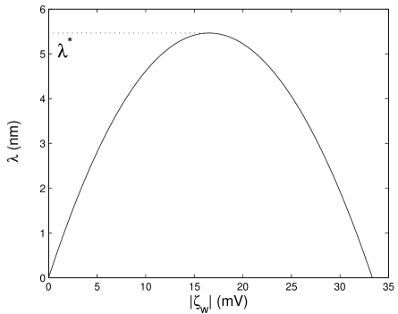
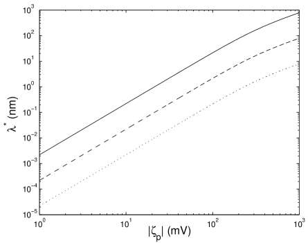
Figure 2: Left: variation of the apparent slip length $\lambda$ (30) for pure water as a function of the wall zeta potential $\zeta_{w}$ for $\zeta_{p}=50$ mV, $n_{0}=10^{-6}$ mol l^-1 (pure water), $\kappa h=10$ and $\kappa a\ll 1$; the slip length reaches a maximum $\lambda^{*}$ for $\zeta_{w}=\zeta_{w}^{*}$. Right: maximum value of the apparent slip length $\lambda^{*}$ as a function of the particle zeta potential $\zeta_{p}$ for $\kappa h=10$, $\kappa a\ll 1$ and three values of the ionic strength: $n_{0}=10^{-6}$ mol l^-1 (pure water, $\kappa^{-1}\approx 300$ nm, solid line), $n_{0}=10^{-4}$ mol l^-1 ($\kappa^{-1}\approx 30$ nm, dashed line), $n_{0}=10^{-2}$ mol l^-1 (tap water, $\kappa^{-1}\approx 3$ nm, dotted line).

4.2 Order of magnitude for water

Let us address here the case of water at room temperature (T=300^∘C, $\epsilon$=80, $\ell\approx 2$ Å). We have calculated numerically the maximum apparent slip lengths which could be obtained in an experiment, $\lambda^{*}$, as a function of the particle zeta potential $\zeta_{p}$. The results are displayed in Figure 2 (right). We first note that $\lambda^{*}$ increases with $|\zeta_{p}|$. Furthermore, the maximum slip length can take values as low as molecular sizes or below and, in the case of pure water, can be as high as hundreds of nanometers.

The data for the low values of $|\zeta_{p}|$ display a power-law behavior, which we can analyze as follows. Let us consider formula (30). The two terms in the denominator will be of the same order of magnitude if $t_{w}$ is larger than a critical value $\tilde{t}_{w}$ which is given by

$$\tilde{t}_{w}\approx\left(\frac{1}{1+\frac{48\pi\ell\epsilon\epsilon_{0}k_{B}T}{e^{2}\kappa h}}\right)^{1/2},$$ (34)

where we have used (33) to relate the conductivity to the screening length. The smallest value of (34) will be obtained, say, for $\kappa h\approx 10$, in which case we get $\tilde{t}_{w}\approx 0.86$ which corresponds to a critical wall zeta potential $\tilde{\zeta}_{w}\approx 135$ mV. Consequently, when $\zeta_{w}\lesssim\tilde{\zeta}_{w}$, (30) can be simplified to

$$\frac{\lambda}{h}=\frac{\zeta_{w}(f(\kappa a)\zeta_{p}-\zeta_{w})(\epsilon\epsilon_{0})^{2}}{\sigma\mu h^{2}},$$ (35)

for which it is easy to get

$$\zeta_{w}^{*}=\frac{f(\kappa a)}{2}\zeta_{p}\,,\quad{\lambda^{*}}=\frac{(\epsilon\epsilon_{0}f(\kappa a)\zeta_{p})^{2}}{4\sigma\mu h}\cdot$$ (36)

The exponent 2 given by equation (36) agrees well with the power-law data presented in Figure 2 (right).

4.3 Comparison with experiments

Two comparisons with experimental results can now be given. First, we wish to comment on the general order of magnitude of the slip lengths obtained. For a review of the pressure-driven flow experiments in capillaries which report some degree of slip as summarized in the introduction, the reader is referred to [36].

The order of magnitude for the maximum slip lengths given by our mechanism (tens to hundreds of nanometers) are consistent with the slip lengths measured in the indirect pressure-driven slip experiments of [6, 8, 10]. Of course, the effect we report here does not directly apply to their pressure drop versus flow rate measurements, but the comparison shows that both effects are comparable in magnitude and therefore the apparent slip mechanism could have important consequences on experimental probing of the no-slip boundary condition.

We also wish to address specifically the experiment of Tretheway & Meinhart [9] for which our study directly applies. The channels used in their experiment have height $2h=30~{}\mu$m and width $2w=300~{}\mu$m; the separation of scale $w\gg h$ allows us to approximate the flow by that between two parallel plates with $h=15$ $\mu$m. Details of the electrical characteristics of the water used in the experiment were not reported, but the water was deionized; we will therefore assume that the ion concentration was small and will take it to be that of pure water $n_{0}\approx 10^{-6}$ mol l^-1 for which $\kappa^{-1}\approx 300$ nm, so that $\kappa h\approx 50$. Particles with radius $a=$150 nm were used in the P.I.V. system, so that $\kappa a\approx 1/2$, for which we will approximate $f(\kappa a)\approx 2/3$. If we assume $|\zeta_{p}|=10$ mV, we obtain that $\lambda^{*}$ is essentially zero. If however $|\zeta_{p}|=50$ mV, we get $\lambda^{*}\approx 1$ nm and $|\zeta_{p}|=200$ mV leads to $\lambda^{*}\approx 18$ nm. Although beyond molecular size, these values are much too small to explain the data reported in [9] where $\lambda\approx 1$ $\mu$m. As a consequence, we can conclude that the effect reported here is probably not responsible for the large slip length observed in [9]. Alternative mechanisms would have to be invoked to explain the data, such as the presence of surface attached bubbles [36].

5 Conclusion

We have reported in this paper the following new mechanism. When small charged colloidal particles are used in a pressure-driven flow experiment to probe the profile of the velocity field of an electrolyte solution (e.g. P.I.V. in water), their velocities may include an “apparent slip” component even though the velocity field in the fluid does not violate the no-slip boundary condition. This apparent slip is in fact an electrophoretic velocity for the particles which are subject to the streaming potential, i.e., the flow-induced potential difference that builds up along the channel due to the advection of free screening charges by the flow. A similar effect is expected to occur in shear-driven flows.

The expected maximum orders of magnitude for the apparent slip lengths were given under normal conditions in water. Although the effect was found to be too small to explain the data reported in [9], its magnitude is consistent with other indirect investigations of fluid slip in pressure-driven flow experiments. As a consequence, the analysis presented here could be a useful tool for experimentalists by allowing them to estimate quantitatively the importance of this apparent slip in their experiments.

The idea that free passive particles could go faster than the surrounding flowing liquid, although counter-intuitive at first, is in fact not unnatural: a similar phenomenon occurs in electrophoresis where, beyond the double layer, the ambient liquid is at rest. We also note from equation (30) and the scalings presented above that the effect increases when the ionic strength of the solution, and therefore its conductivity, decreases; this is because flow of an electrolyte with low ion concentration will necessary lead to the induction of a large streaming electric field to counteract the advection-of-charge electric current.

The model chosen for the calculations used several simplifying assumptions. Our calculations were two-dimensional and we neglected in the model the effect of surface conductance as well as interactions between particles. We also assumed that the streaming electric field was uniform on the length scale of the particle and its double layer. We do not expect that relaxing these assumptions would change qualitatively the physical picture introduced in this paper.

References

- [1] Batchelor, G.K. 1967 Introduction to Fluid Dynamics. Cambridge University Press, Cambridge.
- [2] Goldstein S. 1938 Modern Development in Fluid Dynamics, vol. II, 677-680, Clarendon Press, Oxford.
- [3] Richardson, S. 1973 J. Fluid Mech. 59, 707-719.
- [4] Jansons, K.M. 1988 Phys. Fluids 31, 15-17.
- [5] Schnell, E. 1956 J. Appl. Phys. 27, 1149-1152.
- [6] Churaev, N.V., Sobolev, V.D. & Somov, A.N. 1984 J. Colloid. Int. Sci. 97, 574-581.
- [7] Watanabe, K., Udagawa, Y., & Udagawa, H. 1999 J. Fluid Mech. 381, 225-238.
- [8] Cheng, J.-T. & Giordano, N. 2002 Phys. Rev. E 65, 031206.
- [9] Tretheway, D.C. & Meinhart, C.D. (2002) Phys. Fluids 14, L9-L12.
- [10] Choi, C.-H., Johan, K., Westin, A. & Breuer, K.S. 2003 Phys. Fluids 15, 2897-2902.
- [11] Pit, R., Hervert, H. & Léger, L. 2000 Phys. Rev. Lett. 85, 980-983.
- [12] Baudry, J. & Charlaix, E. 2001 Langmuir 17, 5232-5236.
- [13] Craig, V.S.J., Neto, C. & Williams, D.R.M. 2001 Phys. Rev. Lett. 87, 054504.
- [14] Bonaccurso, E., Kappl, M. & Butt, H.-S. 2002 Phys. Rev. Lett. 88, 076103.
- [15] Cottin-Bizonne, C., Jurine, S., Baudry, J., Crassous, J., Restagno, F. & Charlaix, É. 2002 Eur. Phys. J. E 9, 47-53.
- [16] Zhu, Y. & Granick, S. 2001 Phys. Rev. Lett. 87, 096105.
- [17] Zhu, Y. & Granick, S. 2002 Phys. Rev. Lett. 88, 106102.
- [18] Bonaccurso, E., Butt, H.-S. & Craig, V.S.J. 2003 Phys. Rev. Lett. 90, 144501.
- [19] Thompson, P.A. & Troian, S.M. 1997 Nature 389, 360-362.
- [20] Barrat, J.-L. & Bocquet, L. 1999 Phys. Rev. Lett. 82, 4671-4674.
- [21] Navier, C.L.M.H. 1823 Mémoires de l’Académie Royale des Sciences de l’Institut de France VI, 389-440.
- [22] Leger, L. 2003 C.R. Phys. 4, 241-249.
- [23] Russel, W.B., Saville, D.A. & Schowalter, W.R. 1989 Colloidal Dispersions. Cambridge University Press, Cambridge.
- [24] Burgeen, D. & Nakache, F.R. 1964 J. Phys. Chem. 68, 1084-1091.
- [25] Rice, C.L. & Whitehead, R. 1965 J. Phys. Chem. 69, 4017-4024.
- [26] Levine, S., Marriott, J.R., Neale, G. & Epstein, N. 1975 J. Colloid. Int. Sci. 52, 136-149.
- [27] Hunter R.J. 1982 Zeta potential in colloid science, principles and applications. Academic Press, New York.
- [28] Probstein R.F. 1994 Physicochemical Hydrodynamics: An Introduction John Wiley & Sons, New York.
- [29] Israelachvili, J. 1992 Intermolecular and Surface Forces Academic Press, London.
- [30] Happel, J.R. & Brenner, H. 1965 Low Reynolds Number Hydrodynamics Prentice Hall, Englewood Cliffs, NJ
- [31] Hinch, E.J. 1988 Hydrodynamics at low Reynolds numbers: a brief and elementary introduction, in Disorder and mixing, ed. E. Guyon, J.-P. Nadal, and Y. Pomeau (Kluwer Academic), 43-55.
- [32] Saville, D.A. 1977 Ann. Rev. Mech. 9, 321-337.
- [33] Keh, H.J & Anderson, J.L. 1985 J. Fluid Mech. 153, 417-439.
- [34] Ennis, J. & Anderson, J.L. (1997) J. Colloid Interface Science 185, 497-514.
- [35] Yariv, E. & Brenner, H. (2003) J. Fluid Mech 484, 85 - 111.
- [36] Lauga, E. & Stone, H.A. 2003 J. Fluid Mech. 489, 55-77.