Dynamic tunnelling ionization of H${}_{2}^{+}$ in intense fields

Abstract

Intense-field ionization of the hydrogen molecular ion by linearly-polarized light is modelled by direct solution of the fixed-nuclei time-dependent Schrödinger equation and compared with recent experiments. Parallel transitions are calculated using algorithms which exploit massively parallel computers. We identify and calculate dynamic tunnelling ionization resonances that depend on laser wavelength and intensity, and molecular bond length. Results for $\lambda\sim 1064$ nm are consistent with static tunnelling ionization. At shorter wavelengths $\lambda\sim 790$ nm large dynamic corrections are observed. The results agree very well with recent experimental measurements of the ion spectra. Our results reproduce the single peak resonance and provide accurate ionization rate estimates at high intensities. At lower intensities our results confirm a double peak in the ionization rate as the bond length varies.

The mechanism of high-intensity ionization by infrared and optical wavelength light is often considered a static tunnelling process. The simplicity of this model is hugely appealing because of the ease of calculation. The ionization rates are effectively independent of wavelength, and to some extent the internal structure of the molecule can be ignored [1]. A rough criterion for validity of this model is given by the Keldysh parameter, $\gamma_{k}\equiv\sqrt{|E_{i}|/2U_{p}}$, where the internal binding energy is ($|E_{i}|$) and the external laser-driven kinetic energy is ($U_{p}$). When the conditions are such that $\gamma_{k}\ll 1$, the ionization process is dominated by static tunnelling in which the shape of the potential strongly (exponentially) affects the ionization rate. At certain critical distances between the nuclei, discovered by Codling and co-workers [2], the ionization rate can rise sharply producing a sequence of fast fragments ions at sharply-defined energies. Predictions for ion yields and energies based on classical arguments [1] agree very well with experiments even for large diatomic molecules such as I₂. The presence of critical distances would be evident in polyatomic molecules and is also seen in small rare-gas clusters [3]. The tunnelling process is generally relatively fast compared to the vibrational motion of the molecule, so the fixed-nuclei approximation is reasonable. However the tunnelling time may be longer than the optical period of the laser. Under these conditions the process is more accurately termed a dynamic tunnelling process. In this paper we provide evidence of just such effects for Ti:Sapphire light $\lambda\sim 790$ nm at intensities $I\sim 10^{14}$ W cm^-2. Our theoretical results in this wavelength region do not agree with cycle-averaged static field models, however the results do agree well with the features observed in experimental studies.

In a molecule with few electrons the ionization process can be studied quantally with few approximations. For one-electron models, static-field ionization resonances in the potential wells  [4, 5, 6, 7] occur at distances far from the equilibrium internuclear separation and tend to produce low-energy ions. Experiments have confirmed the existence of enhanced multiphoton ionization in the hydrogen molecular ion at infrared wavelengths [9, 10] but at intensities such that dynamic effects of the field cannot be neglected [11]. The well-established Fourier-Floquet analysis [6, 12] is not particularly suitable for the study of long-wavelength excitations as the number of frequency components required is very large. Moreover, this approach supposes continuous wave conditions such that the state decays exponentially from an isolated resonance state with a lifetime longer than the optical cycle or natural orbital period. Conversely, long-wavelength pulses can be described by quasistatic fields under the conditions such that $\gamma_{k}\ll 1$. However, simple tunnelling formulae assume exponential decay from a single isolated resonance connected adiabatically to the field-free state. This neglects nonadiabatic transitions within the well [7, 13] and rescattering of the continuum electron [14, 15]. Given these difficulties, the direct solution of the Schrödinger equation has distinct advantages. It is suited for all intensities and electronic states and all wavelengths and pulse shapes. In particular it is capable of describing pulse-shape effects and nonadiabatic transitions. Thus it is highly appropriate for realistic modelling of experiments at infrared wavelengths such that $\gamma_{k}\sim 1$.

Tunable Ti:Sapphire light $\lambda\sim 780-800$ nm interacting with atomic hydrogen for example, achieves the pure tunnelling regime, $\gamma_{k}\approx 0.1$, only for intensities $I>1\times 10^{16}$W cm^-2, while for $\lambda=800$ nm with $I\sim 3\times 10^{14}$W cm^-2 [9], $\gamma_{k}\sim 0.7$. Under these latter conditions the ionization rate is well-defined, however a static tunnelling model is unlikely to give a correct estimate of the resonance positions and rates; we show that this is indeed the case. In fact, the dynamic effects displace the critical distances, change the ionization rates, and create electron excitation resonances. In the present work we solve the electronic dynamics exactly by a direct solution of the time-dependent Schrödinger equation (TDSE). This does not include broadening due to the finite focal volume and the corrections due to nuclear motion. Using atomic units, the ground state of the molecular ion is characterized by a bond length $R_{\rm e}=2.0$ and rotational constant $B_{\rm e}=1.36\times 10^{-4}$. If the laser pulse duration is relatively short ($\sim 20$ fs compared with rotational timescale for this molecule ($T_{\rm rot}\sim 1/B_{\rm e}\sim 200$ fs), then the laser-molecule interaction can be regarded as sudden in comparison to the rotation of the system. Neglect of rotation effects is therefore reasonable. In spite of these simplifications the results are very promising and in remarkably good agreement with experiment for the ion energy spectrum. The indications are that appropriate refinements of the model would improve agreement, but this remains a goal for future work.

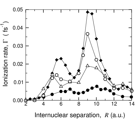
Figure 1: Ionization rate, $\Gamma$, for dynamic and cycled-averaged-static fields. The figure shows the wavelength and bond length dependence of the ionization rate. The maximum field strength $E_{0}=0.05338$ a.u. corresponds to $I=1\times$10¹⁴ W cm^-2. Time-independent cycle-averaged static field rates [6], $\blacklozenge$; time-dependent rates for $\lambda=1064$ nm (this work), $\opencircle$; time-dependent calculations $\lambda$=790 nm (this work), $\opentriangle$; time-dependent rates for $\lambda=1064$ nm [5], $\fullcircle$.

Making these approximations the TDSE, in atomic units, reads

$$H_{\rm e}\Psi_{e}(\bi{r},t)={\rm i}{\partial\over\partial t}\Psi_{e}(\bi{r},t),$$ (1)

where $H_{\rm e}$ is the electronic Hamiltonian and $\Psi_{e}(\bi{r},t)$ the electronic wavefunction. Monochromatic light with linear polarization parallel to the internuclear axis implies a cylindrical symmetry about the internuclear axis with the associated good quantum number $\Lambda$. Thus the electron position can be completely described by the radial, $\rho$, and axial, $z$, coordinates with respect to an origin taken at the midpoint between the nuclei. The TDSE reduces to a 2+1 dimensional partial differential equation where the electronic wavefunction is written as $\Psi_{e}(\rho,z,t)$ and the electronic Hamiltonian takes the form

$$H_{\rm e}(R;\rho,z;t)=-\frac{1}{2}\left(\frac{\partial^{2}}{\partial z^{2}}+\frac{\partial^{2}}{\partial\rho^{2}}+\frac{1}{\rho}\frac{\partial}{\partial\rho}\right)+\frac{\Lambda^{2}}{2\rho^{2}}+V_{\rm e}(R,\rho,z)+V_{\rm m-l}(z,t),$$ (2)

where $R$ is the distance between the two nuclei which have charges $Z_{1}$ and $Z_{2}$, $V_{\rm e}(R,\rho,z)$ is the electronic potential given by

$$V_{\rm e}(R,\rho,z)=-{Z_{1}\over\sqrt{\rho^{2}+(z+\textstyle{1\over 2}R)^{2}}}-{Z_{2}\over\sqrt{\rho^{2}+(z-\textstyle{1\over 2}R)^{2}}}.$$ (3)

and $V_{\rm m-l}(z,t)$ the molecule-laser interaction in the length gauge is given by

$$V_{\rm m-l}(z,t)=zE_{0}f(t)\cos\omega t,$$ (4)

where $E_{0}$ is the peak electric field, $\omega$ the angular frequency and $f(t)$ is the pulse envelope given by

$$f(t)=\left\{\begin{array}[]{lc}\frac{1}{2}\left[1-\cos\left(\frac{\pi t}{\tau_{1}}\right)\right]&0\leq t\leq\tau_{1}\\ 1&\tau_{1}\leq t\leq\tau_{1}+\tau_{2}\\ \frac{1}{2}\left[1-\cos\left(\frac{\pi(t-\tau_{2}-2\tau_{1})}{\tau_{1}}\right)\right]&\tau_{1}+\tau_{2}\leq t\leq\tau_{2}+2\tau_{1}\\ 0&t<0,t>\tau_{2}+2\tau_{1}\end{array}\right.,$$ (5)

where the pulse ramp time is $\tau_{1}$ and the pulse duration $\tau_{2}$, with associated bandwidth $\Delta\omega=1/\tau_{2}$. In the calculations presented in this paper $\tau_{1}=5$ cycles and $\tau_{2}=10$ cycles. It is convenient to change the dependent variable to remove the first-derivative in $\rho$ as follows [16]

$$\phi(\rho,z,t)=(2\pi\rho)^{1/2}\Psi_{e}(\rho,z,t),$$ (6)

so that for $\Sigma$-symmetry ($\Lambda$ = 0) the time-dependent equation is

$$\left[T_{z}+T_{\rho}+V_{\rm m}(\rho,z,R)+V_{\rm m-l}(z,t)\right]\phi(\rho,z,t)={\rm i}\frac{\partial}{\partial t}\phi(\rho,z,t),$$ (7)

where

$$T_{\rho}\equiv-{1\over 2}\left(\frac{\partial^{2}}{\partial\rho^{2}}+\frac{1}{4\rho^{2}}\right)\ \ \ \ \ \ \ \ \ \ \ \ \ \ \ T_{z}\equiv-{1\over 2}\left(\frac{\partial^{2}}{\partial z^{2}}\right),$$ (8)

This 2+1 dimensional TDSE can be discretized on an $N_{\rho}\times N_{z}\times N_{t}$ space-time grid. We label the $N_{\rho}$ radial grid points by, $\{\rho_{1},\rho_{2},\dots\rho_{i},\dots\rho_{N_{\rho}}\}$, while the $N_{z}$ axial grid points are denoted by, $\{z_{1},z_{2},\dots z_{j},\dots z_{N_{z}}\}$. The time evolution progresses through the sequence of times $\{t_{1},t_{2},\dots t_{k},\dots t_{N_{t}}\}$. In this case the wavefunction can be written as the array $\phi(\rho,z,t)\rightarrow\phi(z_{i},\rho_{j},t_{k})$. The method of discretization of the Hamiltonian divides the axial and radial coordinates into subspaces. Two distinct but complementary grid methods are used for the subspaces [16]. The radial subspace is discretized on a semi-infinite range using a small number $N_{\rho}$ of unevenly spaced points that are the nodes of global interpolating functions; Lagrange meshes. This leads to a small dense matrix for the Hamiltonian in the $\rho$-subspace. On the other hand the axial coordinate subspace is represented by a large number of equally-spaced points, with spacing $\Delta z=0.1$ a.u., as lattice points of a finite-difference scheme. The associated subspace Hamiltonian matrix is large but sparse. Our approach is tailored to the requirements of accuracy and computational efficiency. This approach can easily be parallelized to make use of massively parallel processors [14, 16]. At the very least, the dimensions of the cylindrical box, height $2z_{\rm max}$ radius $\rho_{\rm max}$, must be chosen to encompass the tightly-bound states of the system. At the same time the box should be large enough to allow the continuum states to evolve unfettered. As the wavefunction approaches the edge of the box boundaries, we capture the photoelectrons by employing a masking function to absorb the outgoing flux [17]. The ${}^{2}\Sigma^{+}_{\rm g}$ ground state is calculated via an iterative Lanzcos calculation as described in [16].

The quasistatic nature of long-wavelength pulses ($\lambda\sim 1064$ nm) means that it is fair to compare the cycle-average static field ionization rate with the time-dependent ionization rate [7]. The dynamic-field (wavelength-dependent) effects can be judged from figure 1 in which we choose the wavelengths $\lambda=790\rm{nm}$ and $\lambda=1064\rm{nm}$ with the same average intensity $I=1\times$10¹⁴ W cm^-2 ($E_{0}=0.05338$ a.u.). Firstly, for $\lambda=1064\rm{nm}$ the cycle-averaged static field features [6, 7] are very similar to those found using our time-dependent method; with two resonance peaks near $R\sim 5$ a.u. and $R\sim 9$ a.u. However, there are large differences in the shape and relative heights of the peaks. The prominent resonance near $R\sim 9$ a.u. is the charge-resonance peak [13]. The inner peak ($R\sim 5$ a.u.) is a feature of the potential barrier. The longer wavelength $\lambda=1064$ nm does give results very similar to the static cycle-averaged results as expected [6]. For $\lambda\sim 790$ nm, there is a significant reduction in the heights of these peaks and some indication of peak positions moving towards smaller internuclear separations. Calculation at 390nm demonstrate that this trend in peak position moving to smaller values of $R$ is maintained with the first peak found at $R=4$ a.u. for this wavelength. The resonance structure depends on both bond length and wavelength. It is interesting that as the molecule separates into its atomic fragments, the wavelength dependence disappears and the static field result is valid. Figure 1 illustrates very clearly that molecular field ionization differs strongly from atomic field ionization for the bond lengths, wavelengths and intensities of interest. Indeed the molecular ionization rates only converge to within 5% of the atomic rates at $R=20$ a.u. For instance at a wavelength of 1064nm the molecular ionization rate at $R=20$ is $2.85\times 10^{-3}$ fs^-1 compared with the atomic rate of $2.92\times 10^{-3}$ fs^-1. These atomic rates are calculated using the present code which takes $R$=0 and $Z_{1}=Z_{2}=1/2$. These atomic results are in agreement with other accurate time-dependent results [8] to within 0.5%. Our time-dependent results shown in figure 1 for $\lambda=1064$ nm are consistent with previous static field cycle-averaged results [6, 7], although these results disagree with other time-dependent results [5]. There are strong similarities in the $R$ dependence of the rates with those calculated previously. However our rates are up to 4 times higher than those of [5] and the resonance positions are displaced to smaller $R$ values, so that we predict faster ion fragments with higher yields.

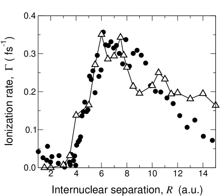
Figure 2: Comparison of ionization rates with experimental measurements at $\lambda$=800 nm, $I=3.2\times$10¹⁴ W cm^-2. The experimental results  [9] ($\fullcircle$) have been normalized to the theoretical calculations ($\opentriangle$).

We apply our model to simulate experiments [9] on the ion energy spectra from the dissociative ionization of the hydrogen molecular ion using $\lambda=800$ nm at $I=3.2\times$10¹⁴ W cm^-2; the results are presented in figure 2. In the experiment an H₂ gas was ionized to form the H${}_{2}^{+}$ ion target. The molecular ions subsequently dissociate and ionize in the laser field, with the proton fragments extracted and energy analyzed. By relating the kinetic energies of the ions to the Coulomb explosion curve, ionization rates could be deduced for the range of molecular bond lengths. The experimental conditions were such that saturation of the ionization channel was avoided, permitting ion yields from larger $R$ values to be estimated and eliminating ion yields from the larger focal volume. Our approximation in assuming a very localized high intensity region, smaller than the diffraction limit, is well justified. The sensitivity of the ionization rate to changes in intensity and wavelength was noted in the results presented in figure 1. Consider the changes in the ionization rates in going from the data presented in figure 1 for $\lambda=790$ nm to that for $\lambda=800$ nm at an intensity 3.2 times higher, in figure 2. The ionization rates in figure 2 are roughly 15 times higher which is consistent with an exponential increase giving rise to more easily measurable ion yields. However the double peak structure of figure 1 is now dominated by a single broad maximum near $R\sim 7$. In comparing with experiment we have in figure 2 normalized the laboratory data to our results. We see that the shape of the theory and experimental curves are in remarkable agreement, in spite of the assumptions made. The single broad peak is reproduced rather well, although some additional structure present in the simulations is not resolved by experiment. For $R>8$ the theory and experiment are in disagreement, and the theoretical estimate of ion yield from $R\sim 9$ is much lower than the experimental results. This might be attributed in part to the variation in focal volume intensity. At the edges of the focal spot the intensities decrease but the interaction volume is larger [1]. Moreover at lower intensities the field ionization rates move to larger $R$ [6]. So one would expect that an inclusion of focal volume variation would broaden the peak to larger values of $R$ and partially compensate for this shortfall. The second feature is that the theoretical results predict high ionization far in excess of that found experimentally at large $R$. The $R\rightarrow\infty$ atomic limit of the theory results is very accurately known and consistent with the theoretical results in figure 2. The theoretical data for ionization rates can be considered as accurate. However the lower ion yield observed can be explained by the fact that during molecular dissociation the molecular ion can ionize at smaller $R$ values. If the ionization rates are large at small $R$, then few if any molecules can survive to be ionized at large bond lengths. A rough estimate of the survival probability $P(R)$ of the molecular ion can be found from the classical dynamics of the ionized molecular ion. The depletion rate is given by $dP/dR\approx-(\Gamma/v)P$ where $v(R)$ is the classical relative velocity of the protons such that $m_{p}v^{2}/4+Z_{1}Z_{2}/R=Z_{1}Z_{2}/R_{e}$ and $m_{p}$ is the proton mass. For the case $\lambda=800$ nm and $I=3.2\times 10^{14}$ Wcm^-2 a rough estimate based on this model gives $P\approx 0.2$ at $R=14$. This is only an indication of the effect but it is consistent with the findings of Dundas [15].

Very recently data have become available from experiments in Garching on H${}_{2}^{+}$ for $\lambda=790\rm{nm}$ at intensities just above the Coulomb explosion threshold, namely $I=0.6\times 10^{14}$ W cm^-2 [18]. In these results the first observations of vibrationally resolved structure has been obtained. From the ion momentum distribution, it was suggested that a critical distance around $R=12$ could explain the results. Existing static field cycle-average rates at a comparable intensity $I=0.56\times 10^{14}$W cm^-2, $E_{0}=0.04$ a.u. [6] are shown in figure 3. These results confirm that the ionization rates are extremely small, the reduction in intensity by a factor of 5 leading to ion yields roughly one hundred times smaller. The double peak structure emerges in our calculations, and since the rates are now reduced, the bulk of the molecules will reach the outer resonance position. In figure 3 the time-dependent calculations for $\lambda$=790 nm and $I=0.6\times 10^{14}$W cm^-2 are in fairly good agreement with the static field results. However we note (figure 3) the inner peak $R\sim 6-8$ is broad and high and ought to produce ion yields comparable to the sharp outer peak near $R=11$. The observation of quantal vibrational structure in the ion spectrum means that a full quantum treatment of nuclear dynamics is required to analyze these new experiments in full.

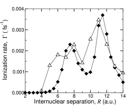
Figure 3: Comparison of ionization rates from the present time-dependent calculations ($\opentriangle$) at $\lambda$=790 nm and $I=0.6\times 10^{14}$W cm^-2 ($E_{0}=0.041$ a.u.) with static field cycle-average rates [6] ($\blacklozenge$) at a comparable intensity of $I=0.56\times 10^{14}$W cm^-2 $E_{0}=0.040$ a.u.

We have solved the full-dimensional TDSE for the electron dynamics of H${}_{2}^{+}$ in linearly polarized laser fields, assuming that the nuclei are fixed in space. The method employed is highly accurate and can be efficiently implemented on parallel processing computers. Ionization rates can be calculated for all nuclear separations and for wavelengths from the infrared to x-ray, for a range of laser pulses. Comparison of our results with other theoretical calculations and recent experimental measurements show very good agreement. We have been able to identify and calculate dynamic tunnelling resonances for $\lambda=790$ nm and $\lambda=800$ nm and obtain accurate estimates of the ionization rates and large dynamic tunnelling corrections are observed. A major simplification in the model is the fixed-nuclei assumption. However, our results for $\lambda=800$ nm and $I=3.2\times 10^{14}$ W cm^-2 reproduce the measured dependence of ionization rate on bond length. At shorter wavelength and lower intensities, $\lambda=790$ nm and $I=0.6\times 10^{14}$ W cm^-2, our results indicate a double peak structure in the ionization rate as the bond length varies. The outer ionization resonance agrees with experimental measurements [18].

To model the experiments more realistically several extensions to the current approach are required. Firstly, the energy and angular momentum exchanges between the nuclei and electrons will occur during process. Dundas [15] has combined the full electronic dynamics with a quantal vibrational motion for intense field dissociative ionization and found that the dynamic tunnelling resonances dominate strongly over pure dissociation at high intensities. A classical model of nuclear motion will not be sufficient as the wavepacket will disperse during the process and indeed experiments are now able to resolve the vibrational structure in the ion yield [18]. The quantal motion is essential to obtain an ion spectrum distribution rather than one-to-one mapping of ion energies to specific bond lengths. Secondly, within the laser focal spot, there is a spatial variation of intensity which has to be taken into account above the saturation intensity. Thirdly, while present calculations only consider parallel electronic transitions, we must consider results averaged over molecular orientation. Previous work by Plummer and McCann [12] found that DC ionization rates decrease sharply as the angle of orientation of the the molecular axis with the field increases. The orientation dependence of dynamic tunnelling ionization has yet to be established. These refinements are likely to be more important in the very high intensity regime $I\sim 10^{15}$ W cm^-2 rather than the regime $I\sim 10^{14}$ W cm^-2. We intend to undertake refinements of our model to simulate these effects and produce accurate estimates of ion yields and ion energy spectra.

LYP acknowledges the award of a PhD research studentship from the International Research Centre for Experimental Physics, Queen’s University Belfast. DD acknowledges the award of an EPSRC Postdoctoral Fellowship in Theoretical Physics. This work has also been supported by a grant of computer resources at the Computer Services for Academic Research, University of Manchester, provided by EPSRC to the UK Multiphoton, Electron Collisions and BEC HPC Consortium.

References

References

- [1] Posthumus J H 2001 Molecules and Clusters in Intense Laser Fields (Cambridge: Cambridge University Press)
- [2] Codling K and Frasinski L J 1993 J.Phys. B: At. Mol. Opt. Phys. 26 783.
- [3] Siedschlag C and Rost J M 2003 Phys. Rev. A 67 013404.
- [4] Seideman T, Ivanov M Yu. and Corkum P B 1995 Phys. Rev. Lett. 75 2819
- [5] Zuo T and Bandrauk A D 1995 Phys. Rev. A 52 R2511.
- [6] Plummer M and McCann J F 1996 J.Phys. B: At. Mol. Opt. Phys. 29 4625.
- [7] Mulyukov Z, Pont M and Shakeshaft R 1996 Phys. Rev. A 54 4229.
- [8] Parker J S, Moore L R, Smyth E S and Taylor K T 2000 J.Phys. B: At. Mol. Opt. Phys. 33 1057.
- [9] Gibson G N, Li M, Guo C and Neira J 1997 Phys. Rev. Lett. 79 2022.
- [10] Williams I D, McKenna P, Srigengan B, Johnston I M, Bryant W A, Sanderson J H, El-Zein A, Goodworth T R J, Newell W R, Taday P F and Langley A J 2000 J.Phys. B: At. Mol. Opt. Phys. 33 2743.
- [11] Williams I D, Newell W R, Taday P F and Langley A J 2003 Euro. Phys. J. D. In Press
- [12] Plummer M and McCann J F 1997 J.Phys. B: At. Mol. Opt. Phys. 30 L401.
- [13] Mulyukov Z and Shakeshaft R 2001 Phys. Rev. A ,63 053404.
- [14] Dundas D, McCann J F, Parker J S and Taylor K T 2000 J.Phys. B: At. Mol. Opt. Phys. 33 3261
- [15] Dundas D 2003 Euro. Phys. J. D. In press.
- [16] Dundas D 2002 Phys. Rev. A 65 023408.
- [17] Smyth E S, Parker J S and Taylor K T 1998 Comp. Phys. Comm. 114 1.
- [18] Pavic̆ić D, Kiess A, Hänsch T W and Figger H 2003 Euro. Phys. J. D. In press.