Linear and nonlinear properties of Rao-dust-Alfvén waves in magnetized plasmas

Abstract

The linear and nonlinear properties of the Rao-dust-magnetohydrodynamic (R-D-MHD) waves in a dusty magnetoplasma are studied. By employing the inertialess electron equation of motion, inertial ion equation of motion, Ampère’s law, Faraday’s law, and the continuity equation in a plasma with immobile charged dust grains, the linear and nonlinear propagation of two-dimensional R-D-MHD waves are investigated. In the linear regime, the existence of immobile dust grains produces the Rao cutoff frequency, which is proportional to the dust charge density and the ion gyrofrequency. On the other hand, the dynamics of an amplitude modulated R-D-MHD waves is governed by the cubic nonlinear Schrödinger equation. The latter has been derived by using the reductive perturbation technique and the two-timescale analysis which accounts for the harmonic generation nonlinearity in plasmas. The stability of the modulated wave envelope against non-resonant perturbations is studied. Finally, the possibility of localized envelope excitations is discussed.

I Introduction

A wide variety of electrostatic and electromagnetic oscillatory modes are known to propagate in unmagnetized and magnetized plasmas Krall ; Stix . Since more than a decade ago, it has been pointed out, and is now well established, that the presence of heavy charged dust particulates in a plasma may strongly modify the dispersion properties of the known low-frequency modes, and may also introduce novel waves Verheest ; PSbook . For instance, inclusion of the dust particle dynamics in an unmagnetized dusty plasma gives rise to the dust-acoustic waves Rao , while the modification of the plasma constituents’ charge balance is responsible for the dust ion-acoustic waves SSDIAW , characterized by an increased phase speed in comparison with the acoustic speed in an electron-ion plasma without dust. In a magnetized dusty plasma, a variety of new modes have been shown to exist, including modified Alfvén waves PKS1992 propagating along to the direction of the external magnetic field $\mathbf{B}$, as well as the modified magnetoacoustic Rao1993 ; Rao1995 and drift-electromagnetic PKS2003 waves propagating across $\mathbf{B}$.

In this paper, we will focus on the linear and nonlinear properties of the Rao-dust-magnetohydrodynamic (R-D-MHD) waves Rao1995 in two space dimensions. The dispersion characteristics of the two-dimensional (2D) R-D-MHD waves differ from the ordinary magnetosonic waves propagating in a magnetized electron–ion (e–i) plasma; of particular importance is the existence of a novel cutoff frequency due to the presence of charged dust grains, as first reported by Rao in his classic paper Rao1995 . Apart from being interesting from a fundamental point of view, and not so widely studied so far, the R-D-MHD waves have been recently shown PS2003 to be excited by the upper-hybrid waves in a uniform dusty magnetoplasma. Our objective here is twofold: i) to present two-dimensional R-D-MHD modes, ii) to study the amplitude modulation of finite amplitude 2D R-D-MHD waves. Assuming the existence of a uniform external magnetic field and relying on the two-fluid model description, we will calculate analytically the harmonic response of the system to a small displacement from equilibrium, trying to point out the role of the dust. The nonlinear modulation of the wave’s amplitude will then be considered by making use of an appropriate reductive perturbation method redpert ; IKPSDIAW ; IKPSDAW . The R-D-MHD wave stability will then be investigated and the existence of envelope excitations will be discussed.

The manuscript is organized in the following fashion. In Sec. II, we present the governing equations for the R-D-MHD waves. Linearized equations and harmonic solutions are presented in Sec. III. Considering oblique nonlinear amplitude modulations of finite amplitude R-D-MHD waves, we derive the nonlinear Schrödinger equation in Sec. IV. A stability analysis is carried out in Sec. V. Section VI contains a discussion of localized R-D-MHD modes. Our conclusions are highlighted in Sec. VII.

II The model

We consider a three-component fully ionized dusty plasma composed of electrons (mass $m$, charge $e$), ions (mass $m_{i}$, charge $q_{i}=+Z_{i}e$) and heavy charged dust particulates (mass $m_{d}$, charge $q_{d}=s\,Z_{d}e$), henceforth denoted by $e,\,i,\,d$ respectively. Dust mass and charge will be taken to be constant, for simplicity. Note that both negative and positive dust charge cases are considered, distinguished by the charge sign $s=$ sgn $q_{d}=\pm 1$.

The plasma is immersed in a uniform external magnetic field along the $\hat{z}-$direction: $\mathbf{B_{0}}=B_{0}\,\hat{z}$ ($B_{0}=$ const.)

II.1 Evolution equations

Let us consider the MHD system of equations for electrons and ions. The massive dust particles are assumed to be practically immobile (‘frozen’ i.e. $n_{d}\approx n_{d,0}$), since we are interested on timescales much shorter than the dust plasma period ($\sim\omega_{p,d}^{-1}$). The electron/ion number density $n_{i,e}$ and velocity $\mathbf{v}_{i,e}$ are governed by the equations

$$\frac{\partial n_{e}}{\partial t}+\nabla\cdot(n_{e}\,\mathbf{u}_{e})=0\,,$$ (1)

$$\frac{\partial n_{i}}{\partial t}+\nabla\cdot(n_{i}\,\mathbf{u}_{i})=0\,,$$ (2)

$$\mathbf{E}+\frac{1}{c}\mathbf{u_{e}\times B}=0\,,$$ (3)

and

$$m_{i}\,D_{i}\,\mathbf{u_{i}}\,\equiv\,m_{i}\,\biggl{(}\frac{\partial\mathbf{u_{i}}}{\partial t}+\mathbf{u_{i}}\cdot\nabla\mathbf{u_{i}}\biggr{)}\,=\,Z_{i}\,e\,\biggl{(}\mathbf{E}+\frac{1}{c}\mathbf{u_{i}\times B}\biggr{)}\,,$$ (4)

where we have completely ignored the electron inertia, as well as pressure (temperature) effects (for all species $\alpha$); the convective derivative operator: $D_{i}\,\equiv\,\frac{\partial}{\partial t}+\mathbf{u_{i}}\cdot\nabla$ has been defined. $\mathbf{E}$ and $\mathbf{B}$ denote the (total) electric and magnetic fields, $\mathbf{E}=\mathbf{0}+\mathbf{E_{1}}$ and $\mathbf{B}=\mathbf{B_{0}}+\mathbf{B_{1}}$, respectively, i.e. index 0 (1) denotes the external (wave) field components. Throughout this text, we shall assume that $\mathbf{E_{1}}=(E_{1,x},E_{1,y},0)$ and $\mathbf{B_{1}}=(0,0,B_{1})$, where $E_{1,x/y}$ and $B_{1}$ are allowed to depend on $\{x,y,t\}$. The system is closed with Maxwell’s equations; neglecting the displacement current, Ampère’s law reads

$$\mathbf{\nabla\times B}=\,\frac{4\pi}{c}\,\mathbf{J}\equiv\frac{4\pi}{c}\,\sum_{\alpha}q_{\alpha}\,n_{\alpha}\,\mathbf{u_{\alpha}}=\,\frac{4\pi e}{c}\,(Z_{i}\,n_{i}\mathbf{u_{i}}-\,n_{e}\mathbf{u_{e}})$$ (5)

and Faraday’s law is

$$\mathbf{\nabla\times E}=\,-\frac{1}{c}\,\frac{\partial\mathbf{B}}{\partial t}\,.$$ (6)

Note that the condition $\mathbf{\nabla\cdot B}=0$ here reduces to $\partial B/\partial z=0$. At equilibrium, the overall neutrality condition holds

$$n_{e,0}-Z_{i}\,n_{i,0}\,-s\,Z_{d}\,n_{d}\,=\,0\,.$$ (7)

Since we are interested in waves propagating in the direction perpendicular to the magnetic field, will shall assume, throughout this study, that the velocities $\mathbf{u_{\alpha}}$ ($\alpha=e,i$), the wavenumber $\mathbf{k}$ and the electric field $\mathbf{E}$ lie in the $xy-$plane. See that $\mathbf{E}$ is orthogonal to $\mathbf{u_{e}}$ and $\mathbf{B}$, due to (3).

II.2 Reduced system of equations

By eliminating $\mathbf{E}$ in (3), (4), we obtain

$$m_{i}\,D_{i}\,\mathbf{u_{i}}\,=\,Z_{i}\,\frac{e}{c}\,\bigl{(}\mathbf{u_{i}}-\mathbf{u_{e}}\bigr{)}\mathbf{\times B}$$ (8)

which, combined with (5), in order to eliminate $\mathbf{u_{e}}$, i.e.

$$\mathbf{u_{e}}\,=\,Z_{i}\,\frac{n_{i}}{n_{e}}\mathbf{u_{i}}\,-\,\frac{c}{4\pi en_{e}}\,\mathbf{(\nabla\times B)}$$ (9)

yields

$$m_{i}\,D_{i}\,\mathbf{u_{i}}\, = \,Z_{i}\,\frac{q_{d}n_{d}}{n_{e}c}\,(\mathbf{u_{i}\times B})\ +\,\frac{Z_{i}}{4\pi n_{e}}\,\mathbf{(\nabla\times B)\times B}$$ (10)

$$= \,Z_{i}\,\frac{q_{d}n_{d}}{n_{e}c}\,(\mathbf{u_{i}\times B})\ +\,\frac{Z_{i}}{4\pi n_{e}}\,\biggl{[}\mathbf{B\cdot\,\nabla B}-\frac{1}{2}\,\mathbf{\nabla}B^{2}\biggr{]}\,,$$

where we have used the quasineutrality condition, $n_{e}-Z_{i}\,n_{i}\,-s\,Z_{d}\,n_{d}\,=\,0$. We observe that, to a first approximation, i.e. assuming very weak magnetic field non-uniformity, the ions (and the electrons due to (9)) are subjected to a rotation due to the presence of charged dust grains, as also shown in Ref. Rao1995 ; PKS2003 : notice the Lorentz centripetal force in the right-hand-side of (10), associated with a rotation frequency which is directly proportional to the dust charge $q_{d}$ (and vanishes without it).

Now, by eliminating $\mathbf{E}$ in (3), (6) and using (9), we obtain

$$\frac{\partial\mathbf{B}}{\partial t}\,=\,\mathbf{\nabla\times}\,\biggl{[}\frac{Z_{i}n_{i}}{n_{e}}(\mathbf{u_{i}\times B})\biggr{]}\,-\,\frac{c}{4\pi e}\,\mathbf{\nabla\times}\,\biggl{[}\frac{1}{n_{e}}(\mathbf{\nabla\times B})\mathbf{\times B}\biggr{]}\,.$$ (11)

Note that Eqs. (8) – (11) lead to a novel low-frequency electromagnetic mode, associated with the presence of charged dust grains, as was recently shown in Ref. PKS2003 ; cf. Eqs. (4), (6) – (8) therein.

The system of equations (10), (11) is not closed in $\mathbf{B}$ and $\mathbf{u_{i}}$, since it also involves $n_{e}$ and $n_{i}$ (both variable), unless one limits the analysis to small (first order) perturbations from equilibrium. Otherwise, for a consistent description, one should either use the complete system of Eqs. (1) – (6) or retain Eqs. (1), (3), (5), (6) and (8) instead. In the following, we will adopt the former option.

The set of equations (1) to (6) is a closed system describing the evolution of the state vector $\mathbf{S}=(n_{e},\,n_{i},\,\mathbf{u_{e}},\,\mathbf{u_{i}},\,\mathbf{E},\,\mathbf{B})$. By assuming that no other vector quantity has a component along the magnetic field $\mathbf{B}=B\,\hat{z}=(B_{0}+B_{1})\,\hat{z}$, viz. $\mathbf{E}=\mathbf{0}+\mathbf{E_{1}}\,=\,(E_{x},E_{y},0)$, and $\mathbf{u_{e/i}}=(u_{e/i,x},u_{e/i,y},0)$,  where $E_{x/y},u_{x/y}$ and $B_{1}$ are functions of $\{x,y;t\}$, we obtain

$$\frac{\partial n_{e}}{\partial t}+\frac{\partial}{\partial x}(n_{e}\,u_{e,x})+\frac{\partial}{\partial y}(n_{e}\,u_{e,y})=0\,,$$ (12)

$$\frac{\partial n_{i}}{\partial t}+\frac{\partial}{\partial x}(n_{i}\,u_{i,x})+\frac{\partial}{\partial y}(n_{i}\,u_{i,y})=0\,,$$ (13)

$$E_{x}=-\frac{1}{c}\,u_{e,y}\,B\,,$$ (14)

$$E_{y}=+\frac{1}{c}\,u_{e,x}\,B\,,$$ (15)

$$m_{i}\,\biggl{(}\frac{\partial}{\partial t}+u_{i,x}\frac{\partial}{\partial x}+u_{i,y}\frac{\partial}{\partial y}\biggr{)}u_{i,x}\,=\,Z_{i}\,e\,\biggl{(}E_{x}+\frac{1}{c}u_{i,y}B\biggr{)}\,=\,\frac{Z_{i}eB}{c}\,\bigl{(}u_{i,y}-u_{e,y}\bigr{)}\,,$$ (16)

$$m_{i}\,\biggl{(}\frac{\partial}{\partial t}+u_{i,x}\frac{\partial}{\partial x}+u_{i,y}\frac{\partial}{\partial y}\biggr{)}u_{i,y}\,=\,Z_{i}\,e\,\biggl{(}E_{y}-\frac{1}{c}u_{i,x}B\biggr{)}\,=\,-\frac{Z_{i}eB}{c}\,\bigl{(}u_{i,x}-u_{e,x}\bigr{)}\,,$$ (17)

$$\frac{\partial B}{\partial y}\,=\,\frac{4\pi e}{c}\,\bigl{(}Z_{i}n_{i}u_{i,x}-n_{e}u_{e,x}\bigr{)}\,,$$ (18)

$$\frac{\partial B}{\partial x}\,=\,-\frac{4\pi e}{c}\,\bigl{(}Z_{i}n_{i}u_{i,y}-n_{e}u_{e,y}\bigr{)}\,,$$ (19)

and

$$\frac{\partial E_{y}}{\partial x}\,-\,\frac{\partial E_{x}}{\partial y}\,=-\frac{1}{c}\frac{\partial B}{\partial t}\,,$$ (20)

describing the evolution of the 9 scalar quantities: $n_{e}$, $n_{i}$, $u_{e,x/y}$, $u_{i,x/y}$, $E_{x/y}$ and $B$. Note that (14), (15) can be used to eliminate $\mathbf{E}$ in (20), which then becomes

$$\frac{\partial B}{\partial t}\,=-\frac{\partial(u_{e,x}\,B)}{\partial x}\,-\,\frac{\partial(u_{e,y}\,B)}{\partial y}\,.$$ (21)

Equations (12) – (20) will be the basis of the analysis that follows.

III Linearized equations - harmonic solutions

By linearizing around the equilibrium state $\mathbf{S_{0}}=(n_{e,0},\,n_{i,0},\,\mathbf{0},\,\mathbf{0},\,\mathbf{0},\,\mathbf{B_{0}})$ viz. $\mathbf{S}=\mathbf{S_{0}}+\mathbf{S_{1}}$ and assuming linear perturbations of the form: $\mathbf{S_{1}}=\mathbf{\hat{S}_{1}}\,\exp i(\mathbf{kx}-\omega t)\,+c.c.\,=\mathbf{\hat{S}_{1}}\,\exp i(kx+ky-\omega t)\,+c.c.\,$ (‘$c.c.$’ denotes the complex conjuguate) we obtain a new system of (linear) equations for the perturbation amplitudes ${(\hat{S}_{1})}_{j}$. A tedious, yet perfectly straightforward (see in the Appendix), calculation leads to the equations

$$\omega(i\omega v_{x}+\delta\Omega_{c,i}v_{y}) = i\Omega_{c,i}^{2}L^{2}k_{x}(k_{x}v_{x}+k_{y}v_{y})\,,$$

$$\omega(i\omega v_{y}-\delta\Omega_{c,i}v_{x}) = i\Omega_{c,i}^{2}L^{2}k_{y}(k_{x}v_{x}+k_{y}v_{y})\,,$$ (22)

in terms of the ion velocity component amplitudes $v_{j}=\hat{u}_{i1,j}$ ($j=x,y$), where we have defined

- the ion gyrofrequency: $\Omega_{c,i}=\frac{Z_{i}eB_{0}}{mc}$ ,

- the characteristic length: $L=\biggl{(}\frac{m_{i}c^{2}n_{i,0}}{4\pi e^{2}n_{e,0}^{2}}\biggr{)}^{1/2}$ , and

- the (dimensionless) dust parameter: $\delta=\frac{Z_{d}n_{d,0}}{n_{e,0}}=s\biggl{(}1-\frac{Z_{i}n_{i,0}}{n_{e,0}}\biggr{)}$; see that $\delta$ cancels in the dust-free limit [cf. (7)].

Equations (22a, b) constitute a $2\times 2$ homogeneous Cramer (linear) system, in terms of $u_{x}$, $u_{y}$, whose determinant should vanish in order for a non-trivial solution to exist; the wave frequency $\Omega$ and wavenumber $\mathbf{k}$ are thus found to obey the dispersion relation

$$\omega^{2}=\omega_{g}^{2}+C^{2}k^{2}$$ (23)

where $k=(k_{x}^{2}+k_{y}^{2})^{1/2}$; we have defined
- the ‘gap frequency’ $\omega_{g}$

$$\omega_{g}=\frac{Z_{d}n_{d,0}Z_{i}eB_{0}}{n_{e,0}m_{i}c}=\delta\,\Omega_{c,i}$$ (24)

and
- the characteristic velocity $C=\Omega_{c,i}\,L$, given by

$$C^{2}=\frac{Z_{i}^{2}B_{0}^{2}n_{i,0}}{4\pi n_{e,0}^{2}m_{i}}=\biggl{(}\frac{Z_{i}n_{i,0}}{n_{e,0}}\biggr{)}^{2}\frac{B_{0}^{2}}{4\pi n_{i,0}m_{i}}\equiv(1-s\delta)^{2}\,V_{A}^{2}\,,$$ (25)

i.e. $C\,=\,\Omega_{c,i}\,L\equiv(1-s\delta)\,V_{A}$, where $V_{A}=B_{0}/(4\pi n_{i,0}m_{i})^{1/2}$ is the Alfvén speed. Notice the effect of the dust, which results in

- a finite (‘gap’) oscillation frequency at the infinite wavelength ($k\rightarrow 0$) limit, and

- a modified phase speed $v_{ph}=\omega/k\,\,\,\,(\neq v_{g}=C^{2}k/\omega$,  for $\delta\neq 0)$; as a matter of fact, the phase speed $v_{g}$ ($\approx C$ for $\omega\gg\omega_{g}$) is higher (lower) than the Alfvén speed $V_{A}$ in the presence of negative (positive) dust.

Notice that (23) coincides with (9) in Ref. PKS2003 . It should also be pointed out that the existence of both the cutoff frequency $\omega_{g}$ and the modified Alfvén speed $C$, associated with the dust-magnetosonic waves, was predicted for the first time by Rao in his classic paper Rao1995 .

The harmonic perturbation amplitudes $\hat{S}_{1,j}$ may now be calculated. Assuming $\mathbf{k}=(k\cos\theta,\,k\sin\theta)$, one obtains the following relations

$$\hat{n}_{e}\,=\,\frac{n_{e,0}}{B_{0}}\,\hat{B}_{1}\equiv c^{(11)}_{1}\,\hat{B}_{1}\,,$$ (26)

$$\hat{n}_{i}\,=\,\frac{n_{e,0}}{Z_{i}B_{0}}\,\hat{B}_{1}\equiv c^{(11)}_{2}\,\hat{B}_{1}\,,$$ (27)

$$\hat{u}_{e,x}\,=\,\biggl{\{}\omega\cos\theta-\,i\,\Omega_{c,i}^{-1}\,\biggl{[}\frac{n_{e,0}}{Z_{i}n_{i,0}}(\omega^{2}-\Omega_{c,i}^{2})+\Omega_{c,i}^{2}\biggr{]}\sin\theta\biggr{\}}\,\frac{\hat{B}_{1}}{B_{0}k}\equiv c^{(11)}_{3}\,\hat{B}_{1}\,,$$ (28)

$$\hat{u}_{e,y}\,=\,\biggl{\{}\omega\sin\theta+\,i\,\Omega_{c,i}^{-1}\,\biggl{[}\frac{n_{e,0}}{Z_{i}n_{i,0}}(\omega^{2}-\Omega_{c,i}^{2})+\Omega_{c,i}^{2}\biggr{]}\cos\theta\biggr{\}}\,\frac{\hat{B}_{1}}{B_{0}k}\equiv c^{(11)}_{4}\,\hat{B}_{1}\,,$$ (29)

$$\hat{u}_{i,x}\,=\,\frac{n_{e,0}}{Z_{i}n_{i,0}}\,\bigl{[}\omega\,\cos\theta+\,i\,s\delta\Omega_{c,i}\sin\theta\bigr{]}\,\frac{\hat{B}_{1}}{B_{0}k}\equiv c^{(11)}_{5}\,\hat{B}_{1}\,,$$ (30)

$$\hat{u}_{i,y}\,=\,\frac{n_{e,0}}{Z_{i}n_{i,0}}\,\bigl{[}\omega\,\sin\theta-\,i\,s\delta\Omega_{c,i}\cos\theta\bigr{]}\,\frac{\hat{B}_{1}}{B_{0}k}\equiv c^{(11)}_{6}\,\hat{B}_{1}\,,$$ (31)

$$\hat{E}_{x}\,=-\frac{B_{0}}{c}u_{e,y}=\,-\biggl{\{}i\,\Omega_{c,i}^{-1}\,\biggl{[}\frac{n_{e,0}}{Z_{i}n_{i,0}}\,(\omega^{2}-\Omega_{c,i}^{2})+\Omega_{c,i}^{2}\biggr{]}\,\cos\theta+\,\omega\,\sin\theta\biggr{\}}\,\frac{\hat{B}_{1}}{c\,k}\,\equiv c^{(11)}_{7}\,\hat{B}_{1}$$ (32)

and

$$\hat{E}_{y}\,=\frac{B_{0}}{c}u_{e,x}=\,-\biggl{\{}i\,\Omega_{c,i}^{-1}\,\biggl{[}\frac{n_{e,0}}{Z_{i}n_{i,0}}\,(\omega^{2}-\Omega_{c,i}^{2})+\Omega_{c,i}^{2}\biggr{]}\,\sin\theta-\,\omega\,\cos\theta\biggr{\}}\,\frac{\hat{B}_{1}}{c\,k}\,\equiv c^{(11)}_{8}\,\hat{B}_{1}\,$$ (33)

(obviously, $c_{9}^{(11)}=1$). Note that these relations satisfy

$$\mathbf{\hat{E}_{1}\cdot\hat{u}_{e,1}}\,=\,0\,,$$

in agreement with (3); also,

$$\mathbf{k\cdot\hat{u}_{e,1}}\,=\,\frac{Z_{i}n_{i,0}}{n_{e,0}}\,\mathbf{k\cdot\hat{u}_{i,1}}\,=\,\frac{\omega}{B_{0}}\,\hat{B}_{1}\,$$

as expected (see the Appendix) as well as

$$\hat{u}_{i,1}=\biggl{(}1-\frac{\omega^{2}}{\Omega_{c,i}^{2}}\biggr{)}^{-1/2}\,\hat{u}_{e,1}\,,$$

(remember that the amplitudes $u_{e/i,\,x/y}$ are complex) implying that the ions and electrons oscillate in (out of) phase for $\omega$ lower (higher) than $\Omega_{c,i}$, i.e. for wavenumber values $k$ below (above) a threshold $k_{cr}=Z_{i}^{1/2}\frac{\Omega_{p,i}}{c}\bigl{(}\frac{1+s\delta}{1-s\delta}\bigr{)}^{1/2}$ (see that $k_{cr}\rightarrow 0$ in the case of complete electron depletion in the plasma, i.e. $\delta\rightarrow 1$, $s=-1$).

IV Oblique nonlinear amplitude modulation

Let us consider the system (12) – (20), which describes the evolution of the (nine scalar) components of $\mathbf{S}$: $\{n_{e},\,n_{i};\,u_{e,x},\,u_{e,y};\,u_{i,x},\,u_{i,y};\,\,E_{x},\,E_{y};\,B_{1}\}$.

In order to study the amplitude modulation of the R-D-MHD waves presented in the previous section, we will assume small deviations from the equilibrium state $\mathbf{S}^{(0)}=\{n_{e,0},\,n_{i,0};\,0,\,0;\,0,\,0;\,0,\,0;\,B_{0}\}$ by taking

$$\mathbf{S}=\mathbf{S}^{(0)}\,+\,\epsilon\,\mathbf{S}^{(1)}+\,\epsilon^{2}\,\mathbf{S}^{(2)}+\,...=\mathbf{S}^{(0)}\,+\,\,\sum_{n=1}^{\infty}\epsilon^{n}\,\mathbf{S}^{(n)}\,,$$

where $\epsilon\ll 1$ is a smallness parameter. Following the standard multiple scale (reductive perturbation) technique redpert ; IKPSDIAW , we shall consider the stretched (slow) space and time variables

$$\zeta\,=\,\epsilon(x-\lambda\,t)\,,\qquad\tau\,=\,\epsilon^{2}\,t\,,$$ (34)

where $\lambda$, having dimensions of velocity, is a real parameter to be later defined. In order to allow for an oblique amplitude modulation on the R-D-MHD wave, we will assume that all perturbed states depend on the fast scales via the phase $\theta_{1}=\mathbf{k\cdot r}-\omega t=k_{x}x+k_{y}y-\omega t$ only, while the slow scales enter the argument of the $l-$th harmonic amplitude $S_{l}^{(n)}$, allowed to vary only along $x$,

$$\mathbf{S}^{(n)}\,=\,\sum_{l=-\infty}^{\infty}\,\mathbf{S}_{l}^{(n)}(\zeta,\,\tau)\,e^{il(\mathbf{k\cdot r}-\omega t)}\,.$$

The reality condition $\mathbf{S}_{-l}^{(n)}={\mathbf{S}_{l}^{(n)}}^{*}$ is met by all state variables. Note that the (choice of) direction of the propagation remains arbitrary, yet modulation is allowed to take place in an oblique direction, characterized by the angle variable $\theta$. Accordingly, the wave-number vector $\mathbf{k}$ is taken to be $\mathbf{k}=(k_{x},\,k_{y})=(k\,\cos\theta,\,k\,\sin\theta)$. According to these considerations, the derivative operators in the above equations are treated as follows

$$\frac{\partial}{\partial t}\rightarrow\frac{\partial}{\partial t}-\epsilon\,\lambda\,\frac{\partial}{\partial\zeta}+\epsilon^{2}\,\frac{\partial}{\partial\tau}\,,$$

and

$$\mathbf{\nabla}\rightarrow\mathbf{\nabla}+\epsilon\,\hat{x}\,\frac{\partial}{\partial\zeta}\equiv(\nabla_{x}+\epsilon\,\frac{\partial}{\partial\zeta},\,\nabla_{y})\,,$$

i.e. explicitly

$$\frac{\partial}{\partial t}\,A_{l}^{(n)}\,e^{il\theta_{1}}=\biggr{(}-il\omega\,A_{l}^{(n)}\,-\epsilon\,\lambda\,\frac{\partial A_{l}^{(n)}}{\partial\zeta}+\epsilon^{2}\,\frac{\partial A_{l}^{(n)}}{\partial\tau}\biggr{)}\,e^{il\theta_{1}}\,,$$

$$\nabla_{x}\,A_{l}^{(n)}\,e^{il\theta_{1}}=\bigr{(}ilk\cos\theta\,A_{l}^{(n)}\,+\epsilon\,\hat{x}\,\frac{\partial A_{l}^{(n)}}{\partial\zeta}\bigr{)}\,e^{il\theta_{1}}\,,$$

and

$$\nabla_{y}\,A_{l}^{(n)}\,e^{il\theta_{1}}=ilk\sin\theta\,A_{l}^{(n)}\,e^{il\theta_{1}}\,,$$

for any of the components $A_{l,j}^{(n)}$ ($j=1,...,9$) of $\mathbf{S}_{l}^{(n)}$.

By substituting the above expressions into Eqs. (12) – (20) and isolating distinct orders in $\epsilon$, we obtain a set of (nine) reduced equations at each ($n$th-) order, describing the evolution of the (nine) components of $\mathbf{S}^{(n)}$. The system is then solved (for each harmonic $l$), substituted into the subsequent order, and so forth. This is a rather standard procedure in the reductive perturbation method framework redpert ; IKPSDIAW ; IKPSDAW , and we shall not burden the presentation with unnecessary details. The outcome of the long algebraic calculation is presented in the following, while essential details are presented in the Appendix.

The first order ($n=1$) first harmonic ($l=1$) equations are just as described in the previous section. Recall the (parabolic) form of the dispersion relation (23), which arises as a compatibility condition. The amplitudes of the first harmonics of the perturbation, say $A_{1,j}^{(1)}$ ($j=1,...,9$) (i.e. precisely $\hat{A}_{j,1}$ in the previous Section), then come out to be directly proportional to the magnetic field perturbation, viz. $A_{1,j}^{(1)}=c_{j}^{(11)}B_{1}^{(1)}$; the coefficients $c_{j}^{(11)}$ are defined in (26) – (33) above. Only the first harmonics have a contribution at this order; indeed, for $n=1,l=0$, one obtains a ($6\times 6$) linear homogeneous system of equations for the (6 components of) $\mathbf{u_{e}},\mathbf{u_{i}},\mathbf{E}$; interestingly, the determinant $D_{0}^{(1)}\sim\Omega_{c,i}q_{d}^{2}$ is non-zero due to (and only in) the presence of dust, so we obtain the trivial solution for the zeroth-harmonic contribution, $\mathbf{u}_{e,0}^{(1)}=\mathbf{u}_{i,0}^{(1)}=\mathbf{E}_{0}^{(1)}=\mathbf{0}$. In addition, $n_{e,0}^{(1)}=n_{i,0}^{(1)}=B_{0}^{(1)}=0$, as imposed by the ($n=2,l=0$) equations.

IV.1 Second order in $\epsilon$: group velocity, 0th and 2nd harmonics

The second order ($n=2$) equations for the first harmonics provide the compatibility condition: $\lambda\,={\partial\omega}/{\partial k_{x}}=\omega^{\prime}(k)\cos\theta$, which defines $\lambda$ as the group velocity $v_{g}=(C^{2}k/\omega)\,\cos\theta$ (the characteristic velocity $C$ was defined previously). The 2nd-order corrections to the first harmonic amplitudes, say $A_{1,j}^{(2)}$ ($j=1,...,9$), come out to be $A_{1,j}^{(2)}=c_{j}^{(21)}{\partial B_{1}^{(1)}}/{\partial\zeta}$, where the coefficients $c_{j}^{(21)}$ are presented in the Appendix.

As expected, second order harmonic contributions arise in this order; their amplitudes, defined by the equations for $n=2$, $l=2$, are found to be proportional to the square of the first order elements, e.g. in terms of $B_{1}^{(1)}$: $A_{2,j}^{(2)}=c_{j}^{(22)}({B_{1}^{(1)}})^{2}$. The nonlinear self-interaction of the carrier wave also results in the creation of a zeroth harmonic, to this order; its strength is analytically determined by taking into account the $l=0$ component of the 3rd and 4th order reduced equations. The result is conveniently expressed in terms of the square modulus of the ($n=1$, $l=1$) quantities, e.g. in terms of $|B_{1}^{(1)}|^{2}=(B_{1}^{(1)})^{*}\,B_{1}^{(1)}$, viz. $A_{0,j}^{(2)}=c_{j}^{(22)}\,|B_{1}^{(1)}|^{2}$ ($j=1,...,9$); once more, the definitions of $c_{j}^{(22)}$, $c_{j}^{(20)}$ can be found in the Appendix. Notice (see the Appendix) the dependence of the expressions derived in this Section (except those for $n_{e,i}$, $B$, in fact) on the value of $\theta$.

IV.2 Derivation of the Nonlinear Schrödinger Equation

Proceeding to the third order in $\epsilon$ ($n=3$), the equation for $l=1$ yields an explicit compatibility condition to be imposed in the right-hand side of the evolution equations which, given the expressions derived previously, can be cast into the form of the Nonlinear Schrödinger Equation (NLSE)

$$i\,\frac{\partial\psi}{\partial\tau}+P\,\frac{\partial^{2}\psi}{\partial\zeta^{2}}+Q\,|\psi|^{2}\,\psi=0\,.$$ (35)

where $\psi\,\equiv\,B_{1}^{(1)}$ denotes the amplitude of the first-order electric field perturbation. Recall that the ‘slow’ variables $\{\zeta,\tau\}$ were defined in (34).

The dispersion coefficient $P$ is related to the curvature of the dispersion curve as $P\,=\,\frac{1}{2}\,\frac{\partial^{2}\omega}{\partial k_{x}^{2}}\,=\,\frac{1}{2}\,\biggl{[}\omega^{\prime\prime}(k)\,\cos^{2}\theta\,+\omega^{\prime}(k)\,\frac{\sin^{2}\theta}{k}\biggr{]}$; the exact form of P reads

$$P(k)\,=\,\frac{C^{2}}{2\omega^{3}}\,\biggl{(}\omega_{g}^{2}\,\cos^{2}\theta\,+\,\omega^{2}\,\sin^{2}\theta\biggr{)}\,,$$ (36)

which is positive for all values of the angle $\theta$, as expected from the parabolic form of $\omega(\mathbf{k})$.

The nonlinearity coefficient $Q$ is due to the carrier wave self-interaction. It is given by

$$Q=\,\frac{\omega}{4\,B_{0}^{2}\,c^{2}\,e^{2}\,m_{i}\,n_{i,0}^{2}\,\pi\,Z_{i}^{2}(n_{e,0}-Z_{i}n_{i,0})^{2}\,k^{2}}\,\biggl{[}-3m_{i}^{2}c^{4}\,n_{e,0}^{2}n_{i,0}\,k^{4}\,\qquad\qquad\qquad\qquad\qquad$$

$$-32e^{4}\,\pi^{2}\,Z_{i}\,(n_{e,0}-Z_{i}n_{i,0})^{4}\,(n_{e,0}+Z_{i}n_{i,0})\,+4c^{2}e^{2}\,k^{2}\,m_{i}\,\pi\,(n_{e,0}-Z_{i}n_{i,0})^{2}(n_{e,0}^{2}-Z_{i}^{2}n_{i,0}^{2})\biggl{]}\,.$$ (37)

Quite surprisingly, $Q$ comes out to be independent of the angle $\theta$. However, as expected, the presence of charged dust grains in the charge balance equation (7) strongly affects the numerical value of $Q$; notice, in passing, that this expression is not valid in the absence of dust grains (since the denominator then vanishes).

The last expression for $Q$ can be conveniently re-arranged, by making use of appropriate plasma quantities. Let us first define the dust parameter: $\mu=n_{e,0}/(Z_{i}n_{i,0})$; see that: $\mu\,=\,1+s\,({Z_{d}n_{d,0}})/({Z_{i}n_{i,0}})$, due to (7), so a value lower/higher than $1$ corresponds to negative/positive dust charge sign; $\mu$ obviously tends to unity in the absence of dust (in any case, $\mu\geq 0$). Check that $\mu=(1-s\delta)^{-1}$ [or $\delta=s(1-1/\mu)$], where $\delta$ was defined above. By normalizing the wavenumber $k$ as $k=K\,\omega_{p,i}/c\equiv(4\pi n_{i,0}Z_{i}e^{2}/m_{i}c^{2})^{1/2}K$ ($\omega_{p,i}$ is the ion plasma frequency), expression (37) can be cast into an elegant form

$$Q(K,\mu)=\,\frac{[(\mu-1)^{2}+x^{2}]^{1/2}\,Z_{i}^{2}e^{2}}{\mu\,(\mu-1)^{2}\,m_{i}^{2}\,c^{2}\,\Omega_{c,i}\,K^{2}}\,\biggl{[}-3\mu^{2}K^{4}\,+(\mu-1)^{2}(\mu^{2}-2)\,K^{2}-2(\mu-1)^{4}(\mu+1)\biggr{]}\,$$ (38)

($\Omega_{c,i}$ denotes the ion gyrofrequency defined previously). Retaining the approximate long-wavelength (i.e. vanishing wavenumber) behaviour of $Q$, we have

$$Q(K\ll 1,\mu)\approx\,-2\frac{(1-\mu)^{3}(1+\mu)\,Z_{i}^{2}}{\mu\,m_{i}^{2}\,c^{2}\,\Omega_{c,i}\,K^{2}}\,$$ (39)

which is always negative and thus ensures, as we shall see in the following, stability at long wavelengths. Note, for later reference, that the same scaling results in relations (23) and (36) taking, respectively, the reduced forms

$$\omega=\Omega_{c,i}\,\biggl{[}\biggl{(}1-\frac{1}{\mu}\biggr{)}^{2}+\frac{x^{2}}{\mu}\biggr{]}^{1/2}$$ (40)

and

$$P=\frac{c^{2}\,\Omega_{c,i}}{2\,\omega_{p,i}^{2}}\,\frac{1}{\mu^{2}}\,\frac{\biggl{[}\biggl{(}1-\frac{1}{\mu}\biggr{)}^{2}+\frac{x^{2}}{\mu}\,\sin^{2}\theta\biggr{]}}{\biggl{[}\biggl{(}1-\frac{1}{\mu}\biggr{)}^{2}+\frac{x^{2}}{\mu}\biggr{]}^{3/2}}\,.$$ (41)

V Stability analysis

The modulational stability profile of a carrier wave whose amplitude is described by the NLS Equation (35) has long been studied, so only the main results have to be summarized here Newell ; Remo ; Fedele ; IKPSDIAW ; IKPSDAW .

The analysis consists in considering the linear stability of the monochromatic (Stokes’s wave) solution of the NLSE (35) $\psi\,=\,{\hat{\psi}}\,e^{iQ|\psi|^{2}\tau}\,+\,c.c.$. If the product $PQ$ of the NLS coefficients is positive, the wave’s envelope may develop an instability when subject to an external perturbation characterized by a wavenumber $\hat{k}$ lower than $\hat{k}_{cr}=\sqrt{2\frac{Q}{P}}|\hat{\psi}_{0}|$. The instability growth rate $\sigma=|Im\hat{\omega}(\hat{k})|$ then reaches its maximum value for $\hat{k}=\hat{k}_{cr}/\sqrt{2}$, viz. $\sigma_{max}\,=\,|Q|\,|\hat{\psi}_{0}|^{2}$. On the other hand, the wave will be stable for all values of $\hat{k}$ if the product $PQ$ is negative.

In our case, the dispersion coefficient $P$ is positive, so one need only investigate the sign of the nonlinearity coefficient $Q$, which is entirely determined by the quantity in brackets in the right-hand-side of (38); this is in fact a bi-quadratic polynomial of $K$, say $p(K,\mu)$. It is a matter of straightforward algebra to show (and an easy matter to confirm, numerically) that $p(K,\mu)$ (and $Q$) is negative for values of $\mu$ below $\mu_{cr}=25.1146$, i.e. for all values of the wavenumber $x$. Therefore, for negative dust charge ($s=-1$ i.e. $\mu<1$), the wave will always be stable. On the other hand, for positive dust charge ($s=+1$ i.e. $\mu>1$), the wave may become unstable (only) for values of $\mu$ above $\mu_{cr}$ i.e. in the case of positive dust charge concentration $q_{d}n_{d}$ higher than $\approx 24q_{i}n_{i}$ (a very rare situation, physically speaking, which implies a very high ion depletion in the plasma). The numerical value of $Q$, as expressed by relation (39), is roughly depicted in figure 1 versus the wavenumber $K$ and the dust parameter $\mu$. As predicted above, $Q$ (and $PQ$) only reaches positive values for $\mu$ beyond $\approx 25$ and $K$ above $\approx 10$ (i.e. $k>10\omega_{p,i}/c$), which is a hardly ever realizable physical situation. We conclude that the R-D-MHD waves are modulationally stable, in the presence of negatively charged dust grains, and (practically) also for positively charged ones.

VI Localized modes

Different types of envelope excitations (solitons) are known to satisfy Eq. (35); in specific, one finds bright- (dark- or grey-) type solitons, e.g. pulses (holes) for a positive (negative) value of the coefficient product $PQ$ Newell ; Remo ; IKPSDIAW ; IKPSDAW ; Fedele , as already long known from nonlinear optics Newell2 ; Hasegawa . According to the conclusions of the preceding Section, the R-D-MHD waves considered in this study will (in the majority of physically realizable situations) rather favour dark-type localized excitations, i.e. field dips (voids) propagating at a constant profile, thanks to the balance between the wave dispersion and nonlinearity. The analytical form of these excitations, depicted in Fig. 2, reads $\psi(\zeta,\tau)=\sqrt{\rho(\zeta,\tau)}\,e^{i\,\Theta(\zeta,\tau)}$, where

$$\rho=\rho_{0}\,\biggl{[}1-a^{2}\,sech^{2}\biggl{(}\frac{\zeta-u\,\tau}{L}\biggr{)}\biggr{]}\,;$$ (42)

where $a$ is a real parameter measuring the depth of the field void: $0<a<1$ ($a=1$) corresponds to grey (black) solitons; see Fig. 2a (2b). The complex expressions for the parameters $a$ and $\Theta$ in the above expression (as well as related ones for bright solitons) can readily be found in the references Newell ; Remo ; IKPSDIAW ; IKPSDAW ; Fedele ; Newell2 ; Hasegawa and are omitted here. Note, however, that the width $L$ of (both bright- and dark-types of) these localized excitations depends on the maximum amplitude $\rho_{0}$ as $L=\sqrt{2\bigl{|}{P}/({Q\,\rho_{0}})\bigr{|}}$; therefore, we retain that for a given amplitude, the (absolute value of the) coefficient ratio $P/Q$ expresses the square width of the soliton, i.e. a pulse if $PQ>0$ and a hole if $PQ<0$. Inversely, for a fixed width $L$, the quotient $P/Q$ expresses the amplitude (height) of the solitary wave $\rho_{0}$.

In figures 3 – 8 we have depicted the ratio $P/Q$ as expressed by the relations (38), (41), expressed in units, say: $P_{0}/Q_{0}=\biggl{(}\frac{c^{2}\,\Omega_{c,i}}{2\,\omega_{p,i}^{2}}\biggr{)}/\biggl{(}\frac{Z_{i}^{2}e^{2}}{m_{i}^{2}\,c^{2}\,\Omega_{c,i}}\biggr{)}=(m_{i}^{2}c^{4}\Omega_{c,i}^{2})/(2Z_{i}^{2}e^{2}\omega_{p,i}^{2})$. In the presence of negative dust ($\mu<1$, see Fig. 3a), the soliton width is seen to bear lower values (with a maximum for higher $K$) as $\mu$ decreases; therefore, an increase in the concentration of negative dust results in generally narrower excitations, but with a peak at higher wavenumbers $K$. Also, for a given $K$, the width is maximum for a certain value of $\mu$ (see Fig. 3b); the position of the maximum depends only slightly on $\theta$ but rather strongly on $K$ (see Figs. 4a, b). Finally, for a fixed value of $\mu$, the $P/Q$ vs. $K$ curve seems to have a maximum at $\theta=\pi/2$; see Fig. 5: transverse modulation slightly favours higher soliton widths. This maximum moves to higher $K$ with increasing dust (i.e. decreasing $\mu$); cf. Figs. 5a, 5b.

For positive dust ($\mu>1$), see Figs. 6 – 8, we have similar qualitative results, yet generally lower values. Once more, the angle variable does not seem to influence the soliton profile dramatically.

VII Conclusions

In this paper, we have studied the 2D linear and nonlinear propagation of R-D-MHD waves in a uniform cold magnetoplasma composed of electrons, ions, and charged dust grains. The presence of immobile charged dust grains is responsible for the ion rotation and a new cutoff frequency (non-existing in an ordinary e–i plasma), which were reported by Rao in his classic paper Rao1995 . The propagation of the modified dust magnetoacoustic waves is possible due to the finite ion inertia effect. The charged dust modifies the phase speed of the modified magnetosonic waves. Furthermore, we have considered the amplitude modulation of the R-D-MHD waves and have shown that self-interactions among waves result in the harmonic generation and the amplitude modulation of a carrier R-D-MHD wave. The wave envelope has been shown to be stable against perturbations in a wide range of physical parameter spaces. Finally, we have discussed the possibility of localized envelope excitations (mostly of the dark soliton type i.e. localized field dips propagating in the plasma) associated with the nonlinear R-D-MHD.

Appendix A 1st-order perturbation: Derivation of the dispersion relation and 1st-harmonic amplitudes

Consider the system: (12) – (20), which describes the evolution of $\mathbf{S}=(n_{e},\,n_{i},\,\mathbf{u_{e}},\,\mathbf{u_{i}},\,\mathbf{E},\,\mathbf{B})$. By linearizing around the equilibrium state $\mathbf{S_{0}}=(n_{e,0},\,n_{i,0},\,\mathbf{0},\,\mathbf{0},\,\mathbf{0},\,\mathbf{B_{0}})$ viz. $\mathbf{S}=\mathbf{S_{0}}+\mathbf{S_{1}}$ and assuming linear perturbations of the form: $\mathbf{S_{1}}=\mathbf{\hat{S}_{1}}\,\exp i(\mathbf{kx}-\omega t)=\mathbf{\hat{S}_{1}}\,\exp i(kx+ky-\omega t)$, we obtain a new system of (linear) equations for the perturbation amplitudes ${(\hat{S}_{1})}_{j}$:

$$-i\,\omega\,\hat{n}_{e,1}+i\,\mathbf{k}\,(n_{e,0}\,\mathbf{\hat{u}_{e1}})\,=0\,,$$ (43)

$$-i\omega\hat{n}_{i,1}+i\,\mathbf{k}\,(n_{i,0}\,\mathbf{\hat{u}_{i1}})\,=0\,,$$ (44)

$$\hat{E}_{1x}=-\frac{1}{c}\,\hat{u}_{e1,y}\,B_{0}\,,$$ (45)

$$\hat{E}_{1y}=\frac{1}{c}\,\hat{u}_{e1,x}\,B_{0}\,,$$ (46)

$$m_{i}\,\bigl{(}-i\,\omega\,\bigr{)}\hat{u}_{i1,x}\,=\,Z_{i}\,e\,\biggl{(}\hat{E}_{1x}+\frac{1}{c}\hat{u}_{i,y}B_{0}\biggr{)}\,=\,+\frac{Z_{i}eB_{0}}{c}\,\bigl{(}\hat{u}_{i,y}-\hat{u}_{e,y}\bigr{)}\,,$$ (47)

$$m_{i}\,\bigl{(}-i\,\omega\,\bigr{)}\hat{u}_{i1,y}\,=\,Z_{i}\,e\,\biggl{(}\hat{E}_{1y}-\frac{1}{c}\hat{u}_{i,x}B_{0}\biggr{)}\,=\,-\frac{Z_{i}eB_{0}}{c}\,\bigl{(}\hat{u}_{i,x}-\hat{u}_{e,x}\bigr{)}\,,$$ (48)

$$i\,k_{y}\,\hat{B}_{1}\,=\,\frac{4\pi e}{c}\,\bigl{(}Z_{i}n_{i,0}\hat{u}_{i1,x}-n_{e,0}\hat{u}_{e1,x}\bigr{)}\,,$$ (49)

$$i\,k_{x}\,\hat{B}_{1}\,=\,-\frac{4\pi e}{c}\,\bigl{(}Z_{i}n_{i,0}\hat{u}_{i1,y}-n_{e,0}\hat{u}_{e1,y}\bigr{)}\,,$$ (50)

and

$$i\,k_{x}\,\hat{E}_{1,y}\,-\,i\,k_{y}\,\hat{E}_{1,x}\,=\frac{1}{c}\,(i\,\omega)\,\hat{B}_{1}\,,$$ (51)

where only first harmonic terms were retained. Now, eliminating the electron velocity amplitudes from (47) – (50) (i.e. solving for $\hat{u}_{e1,j}$ in the latter two and substituting in the former), one immediately obtains:

$$i\,\omega\,\hat{u}_{i1,x}\,+s\Omega_{c,i}\frac{Z_{d}n_{d,0}}{n_{e,0}}\,\hat{u}_{i1,y}\, = \,i\Omega_{c,i}\frac{c}{4\pi en_{e,0}}\,\hat{B}_{1}\,k_{x}$$

$$i\,\omega\,\hat{u}_{i1,y}\,-s\Omega_{c,i}\frac{Z_{d}n_{d,0}}{n_{e,0}}\,\hat{u}_{i1,x}\, = \,i\Omega_{c,i}\frac{c}{4\pi en_{e,0}}\,\hat{B}_{1}\,k_{y}$$ (52)

(the ion cyclotron frequency $\Omega_{c,i}$ was defined in the text). Also, one may substitute from (45), (46) into (51) in order to obtain:

$$\mathbf{k\cdot\hat{u}_{e1}}=\frac{\omega}{B_{0}}\hat{B}_{1}\,,$$ (53)

and, once more, use (47), (48) to eliminate $\mathbf{u_{e1}}$ in it:

$$\frac{\omega}{B_{0}}\hat{B}_{1}\,=\,\frac{Z_{i}n_{i,0}}{n_{e,0}}\,\mathbf{k\cdot\hat{u}_{i1}}\,.$$ (54)

Now, (52a, b), (54) form a closed system, with respect to $\hat{u}_{i1,j}$ ($j=x,y$) and $\hat{B}_{1}$. In specific, one may solve the latter for $\hat{B}_{1}$ and substitute into the former two; one thus obtains precisely the system of equations (22), along with the definitions mentioned in the text.

On a more systematic basis, one may define the matrix:

$$\mathbf{L}_{0}^{(l)}(\omega,\mathbf{k})=\left(\begin{array}[]{ccccccccc}-il\omega&0&ilk_{x}n_{e,0}&ilk_{y}n_{e,0}&0&0&0&0&0\\ 0&-il\omega&0&0&ilk_{x}n_{i,0}&ilk_{y}n_{i,0}&0&0&0\\ 0&0&0&B_{0}&0&0&c&0&0\\ 0&0&-B_{0}&0&0&0&0&c&0\\ 0&0&0&\Omega_{c,i}&-il\omega&-\Omega_{c,i}&0&0&0\\ 0&0&-\Omega_{c,i}&0&\Omega_{c,i}&-il\omega&0&0&0\\ 0&0&\frac{4\pi e}{c}n_{e,0}&0&-\frac{4\pi e}{c}Z_{i}n_{i,0}&0&0&0&ilk_{y}\\ 0&0&0&-\frac{4\pi e}{c}n_{e,0}&0&\frac{4\pi e}{c}Z_{i}n_{i,0}&0&0&ilk_{x}\\ 0&0&0&0&0&0&-ilk_{y}&ilk_{x}&-i\frac{l\omega}{c}\end{array}\right)\,,$$ (55)

which arises naturally by isolating the $l-$th harmonic terms (at every order $n$) in equations (12) – (20). For instance, for $n=l=1$, the system on top of this Appendix is formally expressed as: $\mathbf{L}_{0}^{(1)}\,\mathbf{S}_{1}^{(l)}\,=\,\mathbf{0}$. Now, the condition $Det\mathbf{L}_{0}^{(1)}=0$ leads exactly to the dispersion relation (23), while the solution of the system is given by (26) – (33) in the text.

Appendix B 2nd-order perturbation: group velocity, 0-th and 2-nd harmonic amplitude corrections

For $n=2$, $l=1$, we obtain the system of equations $\mathbf{L}_{0}^{(1)}\,\mathbf{S}_{1}^{(2)}=\mathbf{R}_{1}^{(2)}$, where $\mathbf{L}_{0}^{(1)}$ was defined in (55) and $\mathbf{R}_{1}^{(2)}$ denotes the vector: $\bigl{(}\lambda c_{1}^{(11)}-n_{e,0}c_{3}^{(11)},\,\lambda c_{2}^{(11)}-n_{i,0}c_{5}^{(11)},\,0,\,0,\,\lambda c_{5}^{(11)},\,\lambda c_{6}^{(11)},\,0,\,-1,\,\frac{1}{c}\lambda-c_{8}^{(11)}\bigr{)}^{T}\,\partial B_{1}^{(1)}/\partial\zeta$. The compatibility condition imposed in order for a solution to exist, can be formulated as the constraint: $Det\mathbf{L}_{m}^{(1)}=0$, where $\mathbf{L}_{m}^{(1)}$ is the matrix obtained by substituting the $m-$th column in $\mathbf{L}_{0}^{(1)}$ by $\mathbf{R}_{1}^{(2)}$. Whichever the choice of $m$ ($=1,2,...,9$), by solving the resulting equation, one readily obtains the definition of $\lambda$ as the group velocity $v_{g}=\partial\omega/\partial k_{x}$ (as defined in the text). One then obtains the solution $S_{1,j}^{(2)}=c_{j}^{(21)}{\partial B_{1}^{(1)}}/{\partial\zeta}$ for (8 of) the elements of $\mathbf{S_{2}}^{(1)}$, in terms of one of them, e.g. of $S_{1,9}^{(2)}=B_{1}^{(2)}$. Assuming, with no loss of generality, that $B_{1}^{(2)}=0$, one obtains for the coefficients $c_{j}^{(21)}$ the expressions:

$$c^{(21)}_{1}\, = \,0$$

$$c^{(21)}_{2}\, = \,0$$

$$c^{(21)}_{3}\, = \,\frac{n_{i,0}\,Z_{i}}{B_{0}^{2}\,e\,n_{e,0}^{2}\,n_{i,0}\,Z_{i}^{2}\,\omega\,k^{2}}\biggl{\{}i\,B_{0}\,e\,Z_{i}\biggl{[}n_{e,0}^{2}(\omega^{2}+\Omega_{c,i}^{2})-2n_{e,0}n_{i,0}Z_{i}\Omega_{c,i}^{2}+n_{i,0}^{2}\Omega_{c,i}^{2}Z_{i}^{2}\biggr{]}\cos^{2}\theta$$

$$\,\qquad\qquad\qquad\qquad\qquad+\,n_{e,0}\,\omega\,\Omega_{c,i}\biggl{[}-i\,c\,m_{i}\,n_{e,0}\,\omega+B_{0}eZ_{i}(Z_{i}n_{i,0}-n_{e,0})\sin 2\theta\biggr{]}\biggr{\}}$$

$$c^{(21)}_{4}\, = \,\frac{1}{2\,B_{0}^{2}\,e\,n_{e,0}^{2}\,n_{i,0}\,Z_{i}^{2}\,\omega\,k^{2}}\biggl{\{}2\,c\,m_{i}\,n_{e,0}^{2}\,\omega\,\bigl{[}n_{e,0}(\omega^{2}-\Omega_{c,i}^{2})+n_{i,0}\Omega_{c,i}^{2}Z_{i}\bigr{]}$$

$$\,\qquad\qquad\qquad\qquad\qquad+B_{0}\,e\,n_{i,0}\,Z_{i}^{2}\biggl{[}4n_{e,0}\,\omega\,\Omega_{c,i}(n_{e,0}-Z_{i}n_{i,0})\cos^{2}\theta$$

$$\qquad\qquad\qquad\qquad\qquad\qquad\,i\,\bigl{[}n_{e,0}^{2}(\omega^{2}+\Omega_{c,i}^{2})-2n_{e,0}n_{i,0}\Omega_{c,i}^{2}Z_{i}+n_{i,0}^{2}\Omega_{c,i}^{2}Z_{i}^{2}\bigr{]}\sin 2\theta\biggr{]}\biggr{\}}$$

$$c^{(21)}_{5}\, = \,\frac{i}{8\,\pi\,m_{i}^{2}\,n_{e,0}\,n_{i,0}\,\omega\,c^{2}\,k^{2}}\biggl{\{}B_{0}\,Z_{i}\,\bigl{[}m_{i}\,n_{i,0}\,c^{2}\,k^{2}+8\,\pi\,e^{2}\,(n_{e,0}-Z_{i}n_{i,0})^{2}\bigr{]}\cos 2\theta$$

$$\qquad\qquad\qquad\qquad\qquad\qquad+c\,m_{i}\,\bigl{[}-B_{0}\,Z_{i}n_{i,0}\,c\,k^{2}+8\pi ie\,n_{e,0}\,\omega\,(n_{e,0}-Z_{i}n_{i,0})\sin 2\theta\biggr{\}}$$

$$c^{(21)}_{6}\, = \,\frac{1}{8\,\pi\,m_{i}^{2}\,n_{e,0}\,n_{i,0}\,\omega\,c^{2}\,k^{2}}\biggl{\{}i\,B_{0}\,Z_{i}\,\bigl{[}m_{i}\,n_{i,0}\,c^{2}\,k^{2}+8\,\pi\,e^{2}\,(n_{e,0}-Z_{i}n_{i,0})^{2}\bigr{]}\sin 2\theta$$

$$\qquad\qquad\qquad\qquad\qquad\qquad+8\pi\,e\,c\,m_{i}\,n_{e,0}\,\omega\,(n_{e,0}-Z_{i}n_{i,0})\cos 2\theta\biggr{\}}$$

$$c^{(21)}_{7}\, = \,\frac{B_{0}}{8\,\pi\,em_{i}^{2}\,n_{e,0}^{2}\,\omega\,c^{3}\,k^{2}}\biggl{\{}-2\,m_{i}^{2}\,n_{e,0}\,\omega\,c^{3}\,k^{2}+\,e\,Z_{i}\biggl{[}-8\pi e\,c\,m_{i}\,n_{e,0}\omega(n_{e,0}-Z_{i}n_{i,0})\cos 2\theta$$

$$\qquad\qquad\qquad\qquad\qquad\qquad-iB_{0}\,Z_{i}\,\bigl{[}m_{i}n_{i,0}\,c^{2}\,k^{2}+8\pi e^{2}\,(n_{e,0}-Z_{i}n_{i,0})^{2}\bigr{]}\sin 2\theta\biggr{]}\biggr{\}}$$

$$c^{(21)}_{8}\, = \,\frac{iB_{0}\,Z_{i}}{8\,\pi\,em_{i}^{2}\,n_{e,0}^{2}\,\omega\,c^{3}\,k^{2}}\biggl{\{}c\,m_{i}\biggl{[}-B_{0}\,c\,k^{2}n_{i,0}\,Z_{i}\,+8\pi ien_{e,0}\,\omega(n_{e,0}-Z_{i}n_{i,0})\sin 2\theta$$

$$\qquad\qquad\qquad\qquad\qquad\qquad+B_{0}\,Z_{i}\,\bigl{[}m_{i}n_{i,0}\,c^{2}\,k^{2}+8\pi e^{2}\,(n_{e,0}-Z_{i}n_{i,0})^{2}\bigr{]}\cos 2\theta\biggr{]}\biggr{\}}$$

$$c^{(21)}_{9}\, = \,0$$ (56)

For $n=2$, $l=0$, we obtain the system of equations $\mathbf{L}_{0}^{(0)}\,\mathbf{S}_{0}^{(2)}=\mathbf{R}_{0}^{(2)}\,|B_{1}^{(1)}|^{2}$ (set $l=0$ in (55) for $\mathbf{L}_{0}^{(0)}$), where $\mathbf{R}_{0}^{(2)}$ is the vector $\bigl{(}0,\,0,\,-c_{4}^{(11)},\,c_{3}^{(11)},\,ik_{y}c_{6}^{(11)}{c_{5}^{(11)}}^{*}+\frac{\Omega_{c,i}}{B_{0}}(c_{6}^{(11)}-c_{4}^{(11)}),\,-ik_{x}c_{6}^{(11)}{c_{5}^{(11)}}^{*}-\frac{\Omega_{c,i}}{B_{0}}(c_{5}^{(11)}-c_{3}^{(11)}),\,\frac{4\pi e}{c}(Z_{i}c_{2}^{(11)}{c_{5}^{(11)}}^{*}-c_{1}^{(11)}{c_{3}^{(11)}}^{*}),\,-\frac{4\pi e}{c}(Z_{i}c_{2}^{(11)}{c_{6}^{(11)}}^{*}-c_{1}^{(11)}{c_{4}^{(11)}}^{*}),\,0\bigr{)}^{T}+c.c.$. The 1st, 2nd and 9th equations are identically satisfied, so the corresponding equations for $n=3,l=0$ have to be “borrowed”. Combining them with the remaining (3rd to 8th) equations here, we obtain

$${n_{e}}_{0}^{(2)}\, = \,\frac{n_{e,0}}{v_{g}}c^{(20)}_{3}\,|B_{1}^{(1)}|^{2}\,,$$

$${n_{i}}_{0}^{(2)}\, = \,\frac{n_{i,0}}{v_{g}}c^{(20)}_{5}\,|B_{1}^{(1)}|^{2}\,,$$

$${u_{e,x}}_{0}^{(2)}\, = \,-\frac{2\omega}{B_{0}^{2}k}\cos\theta\,|B_{1}^{(1)}|^{2}\equiv c^{(20)}_{3}\,|B_{1}^{(1)}|^{2}\,,$$

$${u_{e,y}}_{0}^{(2)}\, = \,-\frac{2\omega}{B_{0}^{2}k}\sin\theta\,|B_{1}^{(1)}|^{2}\equiv c^{(20)}_{4}\,|B_{1}^{(1)}|^{2}\,,$$

$${u_{i,x/y}}_{0}^{(2)}\, = \,\biggl{(}\frac{n_{e,0}}{Z_{i}n_{i,0}}\biggr{)}^{2}{u_{e,x/y}}_{0}^{(2)}\equiv c^{(20)}_{5/6}\,|B_{1}^{(1)}|^{2}\,,$$

$${E_{x}}_{0}^{(2)}\, = \,{E_{y}}_{0}^{(2)}\,=\,{B}_{0}^{(2)}\,=\,0$$ (57)

For $n=2$, $l=2$, we obtain a system of (9) equations in the matrix form: $\mathbf{L}_{0}^{(2)}\,\mathbf{S}_{2}^{(2)}=\mathbf{R}_{2}^{(2)}\,{B_{1}^{(1)}}^{2}$ [set $l=2$ in (55] for $\mathbf{L}_{0}^{(2)}$); the (lengthy) expression of the vector $\mathbf{R}_{2}^{(2)}$ is omitted. Solving for the second-harmonic amplitudes ${S_{j}}_{2}^{(2)}$, we obtain:

$${n_{e}}_{2}^{(2)}\, = \,\frac{n_{e,0}^{2}\,\bigl{[}m_{i}n_{i,0}c^{2}\,k^{2}+4\pi e^{2}(n_{e,0}-n_{i,0}Z_{i})^{2}\bigr{]}}{2\pi e^{2}n_{i,0}Z_{i}B_{0}^{2}(n_{e,0}-n_{i,0}Z_{i})^{2}}\,{B_{1}^{(1)}}^{2}\equiv c^{(22)}_{1}\,{B_{1}^{(1)}}^{2}\,,$$

$${n_{i}}_{2}^{(2)}\, = \,\frac{1}{Z_{i}}c^{(22)}_{1}\,{B_{1}^{(1)}}^{2}\equiv c^{(22)}_{2}\,{B_{1}^{(1)}}^{2}\,,$$

$${u_{e,x}}_{2}^{(2)}\, = \,\frac{c^{3}m_{i}^{3}\,\omega}{3\pi e^{4}\,n_{i,0}\,Z_{i}^{4}\,B_{0}^{5}(n_{e,0}-n_{i,0}Z_{i})^{2}\,k}\,\times$$

$$\biggl{\{}\Omega_{c,i}\,\biggl{[}6\pi\,e\,n_{e,0}^{3}\,\omega^{2}+\pi\,Z_{i}\,e\,n_{e,0}^{2}\,n_{i,0}\,(-4\omega^{2}+\Omega_{c,i}^{2})$$

$$\qquad\qquad+n_{i,0}^{2}\,\Omega_{c,i}\,Z_{i}^{2}(B_{0}\,c\,k^{2}-2\pi en_{e,0}\,\Omega_{c,i})+\pi eZ_{i}^{3}\,\,n_{i,0}^{3}\,\Omega_{c,i}^{2}\biggr{]}\,\cos\theta$$

$$-i\,n_{e,0}\,\omega\,\biggl{[}B_{0}\,c\,k^{2}\,\Omega_{c,i}\,(3n_{e,0}\,+Z_{i}n_{i,0})+\pi\,e\,\bigl{[}-2\,n_{e,0}^{2}(2\omega^{2}+\Omega_{c,i}^{2})$$

$$\qquad\qquad+\,n_{e,0}\,n_{i,0}\,Z_{i}\Omega_{c,i}^{2}+n_{i,0}^{2}\,Z_{i}^{2}\,\Omega_{c,i}^{2}\bigr{]}\biggr{]}\,\sin\theta\biggr{\}}$$

$$\equiv c^{(22)}_{3}\,{B_{1}^{(1)}}^{2}$$

$${u_{e,y}}_{2}^{(2)}\, = \,\frac{c^{3}m_{i}^{3}\,\omega}{3\pi e^{4}\,n_{i,0}\,Z_{i}^{4}\,B_{0}^{5}(n_{e,0}-n_{i,0}Z_{i})^{2}\,k}\,\times$$

$$\biggl{\{}\Omega_{c,i}\,\biggl{[}6\pi\,e\,n_{e,0}^{3}\,\omega^{2}+\pi\,Z_{i}\,e\,n_{e,0}^{2}\,n_{i,0}\,(-4\omega^{2}+\Omega_{c,i}^{2})$$

$$\qquad\qquad+n_{i,0}^{2}\,\Omega_{c,i}\,Z_{i}^{2}(B_{0}\,c\,k^{2}-2\pi en_{e,0}\,\Omega_{c,i})+\pi eZ_{i}^{3}\,\,n_{i,0}^{3}\,\Omega_{c,i}^{2}\biggr{]}\,\sin\theta$$

$$+\,i\,n_{e,0}\,\omega\,\biggl{[}B_{0}\,c\,k^{2}\,\Omega_{c,i}\,(3n_{e,0}\,+Z_{i}n_{i,0})+\pi\,e\,\bigl{[}-2\,n_{e,0}^{2}(2\omega^{2}+\Omega_{c,i}^{2})$$

$$\qquad\qquad+\,n_{e,0}\,n_{i,0}\,Z_{i}\Omega_{c,i}^{2}+n_{i,0}^{2}\,Z_{i}^{2}\,\Omega_{c,i}^{2}\bigr{]}\biggr{]}\,\cos\theta\biggr{\}}$$

$$\equiv c^{(22)}_{4}\,{B_{1}^{(1)}}^{2}\,,$$

$${u_{i,x}}_{2}^{(2)}\, = \,\frac{c^{2}m_{i}^{2}\,n_{e,0}^{2}\,\omega}{3\pi e^{3}\,n_{i,0}^{2}\,Z_{i}^{4}\,B_{0}^{4}(n_{e,0}-n_{i,0}Z_{i})^{2}\,k}\,\times$$

$$\biggl{\{}\biggl{[}B_{0}\,c\,k^{2}\,Z_{i}n_{i,0}\,\omega+\pi\,e\,[n_{e,0}^{2}(2\omega^{2}+\Omega_{c,i}^{2})-2n_{e,0}\,n_{i,0}\,Z_{i}\Omega_{c,i}^{2}\,+Z_{i}^{2}n_{i,0}^{2}\Omega_{c,i}^{2}]\biggr{]}\cos\theta$$

$$\qquad\qquad+3\pi\,i\,e\,n_{e,0}\,\Omega_{c,i}\,\omega\,(n_{e,0}-n_{i,0}Z_{i})\,\sin\theta\biggr{\}}\equiv c^{(22)}_{5}\,{B_{1}^{(1)}}^{2}\,,$$

$${u_{i,y}}_{2}^{(2)}\, = \,\frac{c^{2}m_{i}^{2}\,n_{e,0}^{2}\,\omega}{3\pi e^{3}\,n_{i,0}^{2}\,Z_{i}^{4}\,B_{0}^{4}(n_{e,0}-n_{i,0}Z_{i})^{2}\,k}\,\times$$

$$\biggl{\{}\biggl{[}B_{0}\,c\,k^{2}\,Z_{i}n_{i,0}\,\omega+\pi\,e\,[n_{e,0}^{2}(2\omega^{2}+\Omega_{c,i}^{2})-2n_{e,0}\,n_{i,0}\,Z_{i}\Omega_{c,i}^{2}\,+Z_{i}^{2}n_{i,0}^{2}\Omega_{c,i}^{2}]\biggr{]}\sin\theta$$

$$\qquad\qquad-3\pi\,i\,e\,n_{e,0}\,\Omega_{c,i}\,\omega\,(n_{e,0}-n_{i,0}Z_{i})\,\cos\theta\biggr{\}}\equiv c^{(22)}_{6}\,{B_{1}^{(1)}}^{2}\,,$$

$${E_{x}}_{2}^{(2)}\, = \,-\frac{m_{i}^{2}\,c}{3\pi e^{3}\,n_{i,0}\,Z_{i}^{3}\,B_{0}^{3}(n_{e,0}-n_{i,0}Z_{i})^{2}\,k}\,\times$$

$$\biggl{\{}i\biggl{[}B_{0}c\,k^{2}\,(3n_{e,0}^{2}\omega^{2}+n_{e,0}n_{i,0}Z_{i}\Omega_{c,i}^{2}-n_{i,0}^{2}Z_{i}^{2}\Omega_{c,i}^{2})+$$

$$\pi e\Omega_{c,i}\,(n_{e,0}-n_{i,0}Z_{i})[n_{e,0}^{2}\,(-7\omega^{2}+\Omega_{c,i}^{2})-2\,n_{e,0}n_{i,0}Z_{i}\,\Omega_{c,i}^{2}\,+n_{i,0}^{2}Z_{i}^{2}\,\Omega_{c,i}^{2}]\biggr{]}\cos\theta$$

$$+6\pi\,e\,n_{e,0}^{3}\,\omega^{3}\,\sin\theta\biggr{\}}\equiv c^{(22)}_{7}\,{B_{1}^{(1)}}^{2}$$

$${E_{y}}_{2}^{(2)}\, = \,\frac{m_{i}^{2}\,c}{3\pi e^{3}\,n_{i,0}\,Z_{i}^{3}\,B_{0}^{3}(n_{e,0}-n_{i,0}Z_{i})^{2}\,k}\,\times$$

$$\biggl{\{}-i\biggl{[}B_{0}c\,k^{2}\,(3n_{e,0}^{2}\omega^{2}+n_{e,0}n_{i,0}Z_{i}\Omega_{c,i}^{2}-n_{i,0}^{2}Z_{i}^{2}\Omega_{c,i}^{2})+$$

$$\pi e\Omega_{c,i}\,(n_{e,0}-n_{i,0}Z_{i})[n_{e,0}^{2}\,(-7\omega^{2}+\Omega_{c,i}^{2})-2\,n_{e,0}n_{i,0}Z_{i}\,\Omega_{c,i}^{2}\,+n_{i,0}^{2}Z_{i}^{2}\,\Omega_{c,i}^{2}]\biggr{]}\sin\theta$$

$$+6\pi\,e\,n_{e,0}^{3}\,\omega^{3}\,\cos\theta\biggr{\}}\equiv c^{(22)}_{8}\,{B_{1}^{(1)}}^{2}$$

$${B}_{2}^{(2)}\, = \,\frac{2c^{2}m_{i}^{2}\,n_{e,0}^{3}\,\omega^{2}}{e^{2}\,n_{i,0}\,Z_{i}^{3}\,B_{0}^{3}(n_{e,0}-n_{i,0}Z_{i})^{2}}\equiv c^{(22)}_{9}\,{B_{1}^{(1)}}^{2}\,.$$ (58)

Figure Captions

Figure 1.

The value of the coefficient $Q$ is depicted against the dust parameter $\mu$ and the (normalized) wavenumber $K$.

Figure 2.

Soliton solutions of the NLS equation for $PQ<0$ (holes); these excitations are of: (a) dark type, (b) grey type. Notice that the amplitude never reaches zero in (b). These excitations represent electromagnetic field dips (voids) associated with the nonlinear R-D-MHD wave propagation.

Figure 3.

Negative dust; the (normalized) soliton width $L$ (absolute value of $P/Q$) is depicted: (a) against wavenumber $K$, for $\theta=0$ and $\mu=0.8,0.7,0.6,0.5$ (from top to bottom); (b) against the dust parameter $\mu$, for $K=0.2$ and $\theta=0{}^{\circ},30{}^{\circ},60{}^{\circ},90{}^{\circ}$ (from bottom to top).

Figure 4.

Negative dust; the (normalized) soliton width $L$ (absolute value of $P/Q$) is depicted versus the dust parameter $\mu$ and the angle $\theta$ for: (a) $K=0.2$; (b) $K=0.5$.

Figure 5.

Negative dust; the soliton width $L$ (absolute value of $P/Q$) is depicted versus the wavenumber $K$ and the angle $\theta$ for: (a) $\mu=0.8$; (b) $\mu=0.5$.

Figure 6.

Similar to Fig. 3, for positive dust; the (normalized) soliton width (absolute value of $P/Q$) is depicted: (a) against wavenumber $K$, for $\theta=0$ and $\mu=1.5,2.0,2.5$ (from top to bottom); (b) against the dust parameter $\mu$, for $K=0.2$ and $\theta=0{}^{\circ},30{}^{\circ},60{}^{\circ},90{}^{\circ}$ (from bottom to top).

Figure 7.

Similar to Fig. 4, for positive dust; the (normalized) soliton width (absolute value of $P/Q$) is depicted versus the dust parameter $\mu$ and the angle $\theta$ for: (a) $K=0.2$; (a) $K=0.5$.

Figure 8.

Similar to Fig. 5, for positive dust; the soliton width (absolute value of $P/Q$) is depicted versus the wavenumber $K$ and the angle $\theta$ for: (a) $\mu=1.2$; (b) $\mu=1.5$.

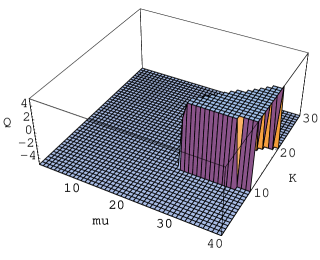
Figure 1:

Figure 2:

Figure 3:

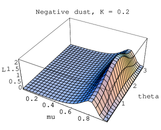
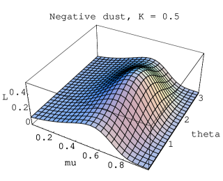
Figure 4:

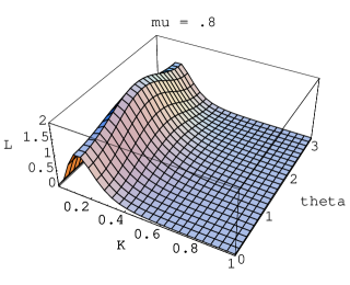
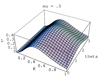
Figure 5:

Figure 6:

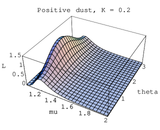
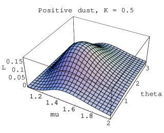
Figure 7:

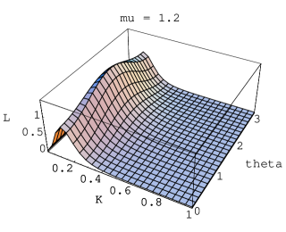
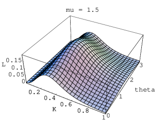
Figure 8:

References

(1) N. A. Krall and A. W.
Trivelpiece, Principles of plasma physics, McGraw - Hill
(New York, 1973).
(2) Th. Stix, Waves in Plasmas, American
Institute of Physics (New York, 1992).
(3) F. Verheest,
Waves in Dusty Space Plasmas (Kluwer Academic Publishers,
Dordrecht, 2001).
(4) P. K. Shukla and A. A. Mamun,
Introduction to Dusty
Plasma Physics (Institute of Physics, Bristol, 2002).
(5) N. N. Rao, P. K. Shukla and M. Y. Yu, Planet. Space
Sci. 38, 543 (1990).
(6) P. K. Shukla and V. P. Silin, Phys. Scr. 45,
508 (1992).
(7) P. K. Shukla, Phys. Scr. 45,
504 (1992).
(8) N. N. Rao, J. Plasma Phys. 49, 375 (1993).
(9) N. N. Rao, J. Plasma Phys. 53, 317 (1995).
(10) P. K. Shukla, Phys. Lett. A 316, 238 (2003).
(11) P. K. Shukla and L. Stenflo,
Phys. Plasmas 10, 4572 (2003).
(12) T. Taniuti and N. Yajima, J. Math. Phys. 10,
1369 (1969);
N. Asano, T. Taniuti and N. Yajima, J. Math. Phys. 10, 2020 (1969).
(13) I. Kourakis and P. K. Shukla,
Phys. Plasmas 10 (9), 3459 (2003).
(14) I. Kourakis and P. K. Shukla,
Physica Scripta 69, in press (2004).
(15) A. C. Newell,
Solitons in Mathematics and Physics
(SIAM, Philadelphia Pennsylvania, 1985).
(16) M. Remoissenet,
Waves Called Solitons (Springer-Verlag, Berlin, 1994).
(17) R. Fedele and H. Schamel, Eur. Phys. J. B27
313 (2002); R. Fedele, H. Schamel and P. K. Shukla, Phys.
Scripta T 98 18 (2002).
(18) A. Hasegawa,
Optical Solitons in Fibers
(Springer Verlag, Berlin, 1989).
(19) A. C. Newell and J. V. Moloney,
Nonlinear Optics
(Addison-Wesley Publ. Co., Redwood City Ca., 1992).