Oblique amplitude modulation of dust-acoustic plasma waves

Abstract

Theoretical and numerical studies are presented of the nonlinear amplitude modulation of dust-acoustic (DA) waves propagating in an unmagnetized three component, weakly-coupled, fully ionized plasma consisting of electrons, positive ions and charged dust particles, considering perturbations oblique to the carrier wave propagation direction. The stability analysis, based on a nonlinear Schrödinger-type equation (NLSE), shows that the wave may become unstable; the stability criteria depend on the angle $\theta$ between the modulation and propagation directions. Explicit expressions for the instability rate and threshold have been obtained in terms of the dispersion laws of the system. The possibility and conditions for the existence of different types of localized excitations have also been discussed.

I Introduction

The study of the dynamics of dust contaminated plasmas (DP) has recently received considerable interest due to their occurrence in real charged particle systems, e.g. in space and laboratory plasmas and the novel physics involved in their description PSbook . An issue of particular interest is the existence of special acoustic-like oscillatory modes, e.g. the dust-acoustic waves (DAW) and dust-ion-acoustic waves (DIAW), which were theoretically predicted about a decade ago Rao ; SSIAW and later experimentally confirmed Barkan ; Pieper . The DAW, which we consider herein, relies on a new physical mechanism in which inertial dust grains oscillate against a thermalized background of electrons and ions which provide the necessary restoring force. The phase speed of the DAW is much smaller than the electron and ion thermal speeds, and the DAW frequency is below the dust plasma frequency.

A long-known generic characteristic of nonlinear wave propagation is amplitude modulation due to the nonlinear self-interaction of the carrier wave, which generates higher harmonics. The standard method for studying this mechanism is a multiple space and time scale technique redpert ; redpert2 , which leads to a nonlinear Schrödinger-type equation (NLSE) describing the evolution of the wave envelope. It has been shown that, under certain conditions, waves may develop a Benjamin-Feir-type (modulational) instability (MI), i.e. their modulated envelope may collapse under the influence of external perturbations. Furthermore, the NLSE-based analysis, already present in a wide variety of contexts Remoissenet ; Sulem ; Hasegawa1 , reveals the possibility of the existence of localized excitations (solitary wave structures) whose form and behaviour depends on criteria similar to the ones necessary for the MI to occur.

Not surprisingly, plasma wave theory has provided an excellent test bed for this approach since a long time ago [7, 11 - 19] and dusty plasma waves were no exception [20 – 22]. Among other noteworthy results, electron plasma modes have been shown to be stable against parallel modulation Kakutani ; so do the ion plasma modes, yet only for perturbations below a specific wavenumber threshold Chan . Electron and ion acoustic modes, even though stable to parallel modulation Kakutani ; Shimizu ; Kako1 ; comment1 , are found to be unstable if one takes into account finite temperature effects Chan ; Durrani ; chin3 or, most interesting to us, when subject to an oblique modulation of the wave amplitude [17 – 19]. These results, based on Poisson - moment plasma equations, have been confirmed by similar studies from a kinetic point of view kinetic , for the ion - acoustic wave in an electron - ion plasma. In dusty plasma, the amplitude modulation of the DAW and DIAW has been investigated in Ref. [20 – 22]; similar studies have been carried out for oscillations in (strongly-coupled) dusty plasma quasi-crystals [25 - 26]. Finally, let us mention that attempts have been made to refine the description of the DIAW modulation by including non-planar geometry effects chin2 , following an idea applied earlier in the KdV (Korteweg-de Vries) description of a dusty plasma MS , and dust-charge fluctuation effects chin , an issue of particular importance in the present-time DP surveys (see e.g. Ivlev ; Mamun ; also PSbook ). These effects, omitted in the present investigation, will be considered in a forthcoming work.

In this paper, we study the modulational instability of dust-acoustic plasma waves propagating in an unmagnetized plasma contaminated by a population of charged dust grains, whose dimensions and charge are assumed constant, for simplicity. Amplitude modulation is allowed to take place in an oblique direction, at an angle $\theta$ with respect to the carrier wave propagation direction. Once an explicit criterion for the occurrence of instability is established, our aim is to trace the influence of $\theta$ on the conditions for the MI onset, and determine the magnitude of the associated instability growth rate. Finally, we shall also examine the possibility of the formation of localized excitations and discuss their characteristics. Exact new expressions are derived for all quantities of interest, in terms of the system’s dispersion laws. Among other physical parameters discussed, our formulation leaves open the choice of sign of dust charge ($sign\,q_{d}=\pm 1$) (most often taken to be negative since this is the most frequently occurring case PSbook ) and the dust pressure (‘temperature’) scaling. Our aim in doing so is to address, among others, the question of the influence of the dust charge sign on the amplitude modulation mechanism. We may also attempt to clarify the effect of taking (or not) into account the dust pressure evolution equation (omitted e.g. in AMS ) in the analysis.

The manuscript is organized as follows. In the next Section, the analytical model is introduced. In Section III, we carry out a perturbative analysis by introducing appropriate slow space and time evolution scales, and derive a NLS-type equation which governs the (slow) amplitude evolution in time and space. The exact form of dispersion and nonlinearity coefficients in the NLS-type equation is presented and discussed. In Section IV, we carry out a stability analysis of the NLSE allowing for a thorough study of the DAW stability in various regions of the physical parameters involved. The analysis is pursued in Section V, where we discuss the possibility of the existence of localized solutions of the NLSE, and identify their forms in different parameter regions. Finally, we briefly summarize our results in the concluding Section.

II The model

We consider a three component collisionless unmagnetized dusty plasma consisting of electrons (mass $m$, charge $e$), ions (mass $m_{i}$, charge $q_{i}=+Z_{i}e$) and heavy dust particulates (mass $m_{d}$, charge $q_{d}=s\,Z_{d}e$), henceforth denoted by $e,\,i,\,d$ respectively. Dust mass and charge will be taken to be constant, for simplicity. Note that both negative and positive dust charge cases are considered, distinguished by the charge sign $s=sgn\,q_{d}=\pm 1$ in the formulae below.

II.1 Evolution equations

The basis of our study includes the moment - Poisson system of equations for the dust particles and Boltzmann distributed electrons and ions. The dust (number) density $n_{d}$ is governed by the (continuity) equation

$$\frac{\partial n_{d}}{dt}+\nabla\cdot(n_{d}\,\mathbf{u}_{d})=0\,,$$ (1)

and the dust mean velocity $\mathbf{u}_{d}$ obeys

$$\frac{\partial\mathbf{u}_{d}}{dt}+\mathbf{u}_{d}\cdot\nabla\mathbf{u}_{d}\,=\,-\frac{q_{d}}{m_{d}}\,\nabla\,\Phi-\frac{1}{m_{d}n_{d}}\,\nabla p_{d}\,,$$ (2)

where $\Phi$ is the electric potential. The dust pressure $p_{d}$ obeys

$$\frac{\partial p_{d}}{dt}+\mathbf{u}_{d}\cdot\nabla p_{d}\,=\,-\gamma\,p_{d}\,\nabla\cdot\mathbf{u}_{d}\,$$ (3)

Here $\gamma=(f+2)/f$ is the ratio of specific heats ($f$ is the number of degrees of freedom) e.g. $\gamma=3$ in the adiabatic one-dimensional (1d) case and $\gamma=2$ in the two-dimensional (2d) case. The system is closed with Poisson’s equation

$$\nabla^{2}\Phi\,=\,-4\pi\,\sum q_{s}\,n_{s}\, = \,4\pi\,(n_{e}\,e-q_{i}\,n_{i}-q_{d}\,n_{d})\equiv\,4\pi\,e\,(n_{e}-Z_{i}\,n_{i}-s\,Z_{d}\,n_{d})\,;$$ (4)

note that the right-hand-side cancels at equilibrium due to the overall neutrality condition

$$n_{e,0}\,e-n_{i,0}\,q_{i}-n_{d,0}\,q_{d}\,=\,0\,.$$ (5)

The right-hand side in (4) is often formulated in terms of the ratio $\mu=n_{e,0}/(Z_{i}n_{i,0})$; for convenience, we have

$$\mu\,=\,1+s\,\frac{Z_{d}}{Z_{i}}\frac{n_{d,0}}{n_{i,0}}$$ (6)

due to (5), so that a value lower (higher) than $1$ corresponds to negative (positive) dust charge; $\mu$ obviously tends to unity in the absence of dust (in any case, $\mu>0$). We will retain this notation in the following, for the sake of reference to previous works.

The electrons and ions are assumed to be close to a Maxwellian equilibrium. The corresponding densities are

$$n_{e}\approx n_{e,0}\,e^{e\Phi/k_{B}T_{e}}\,,$$

and

$$n_{i}\approx n_{i,0}\,e^{-Z_{i}\,e\Phi/k_{B}T_{i}}\,,$$ (7)

where $T_{s}$ denotes the temperature of species $s=e,i$ ($k_{B}$ is the Boltzmann constant).

II.2 Reduced equations

Re-scaling all variables over appropriately chosen quantities and developing around $\Phi=0$, Eqs. (1) - (7) can be cast in the reduced form

$$\frac{\partial n}{dt}+\nabla\cdot(n\,\mathbf{u}) = 0\,,$$

$$\frac{\partial\mathbf{u}}{dt}+\mathbf{u}\cdot\nabla\mathbf{u}\, = \,-s\,\nabla\phi-\frac{\sigma}{n}\,\nabla p\,,$$

$$\frac{\partial p}{dt}+\mathbf{u}\cdot\nabla p\, = \,-\gamma\,p\,\nabla\cdot\mathbf{u}\,,$$

and

$$\nabla^{2}\phi\,=\,\phi-\alpha\,\phi^{2}+\alpha^{\prime}\,\phi^{3}-s\,\beta\,(n-1)\,,$$ (8)

where all quantities are non-dimensional: $n=n_{d}/n_{d,0}$, $\mathbf{u}=\mathbf{u}_{d}/v_{0}$, $p=p_{d}/p_{0}$ and $\phi=\Phi/\Phi_{0}$; the scaling quantities (index $0$) are, respectively: the equilibrium density $n_{d,0}$, the ‘dust sound speed’ $v_{0}=v_{d}=(k_{B}T_{e}/m_{d})^{1/2}$, $p_{0}=n_{d,0}k_{B}T_{e}$ and $\Phi_{0}=(k_{B}T_{e}/Z_{d}e)$. Space and time in (8) are, respectively, scaled over: the DP effective Debye length $\lambda_{D,eff}=(\lambda_{D,e}^{-2}+\lambda_{D,i}^{-2})^{-1/2}$ (where $\lambda_{D,s}=(k_{B}T_{s}/4\pi n_{s,0}q_{s}^{2})^{1/2}$, $s=e,i$) and the inverse DP plasma frequency $\omega_{p,d}^{-1}=(4\pi n_{d,0}q_{d}^{2}/m_{d})^{-1/2}$. Recall that $s=$sgn $q_{d}$, so the influence of the dust charge sign will be traced via the appearance of $s$ in the forthcoming formulae. Finally, $\sigma=p_{0}/(n_{d,0}k_{B}T_{e})$ is equal to unity, given the above choice for $p_{0}$; nevertheless, $\sigma$ - often interpreted as a temperature ratio via a different scaling, see e.g. chin - will be retained in order to ‘tag’ the influence of the coupling to pressure evolution equation (3) being taken into account - as compared to a previous work AMS where Eq. (3) has been omitted. As a matter of fact, expressions (9) - (11) therein are readily recovered here upon setting $\sigma=0$, $s=-1$, $\alpha^{\prime}=0$ in Eq. (8) above.

The dimensionless parameters appearing in (8) are

$$\alpha=\frac{1}{2Z_{d}}\frac{Z_{i}^{3}(\frac{T_{e}}{T_{i}})^{2}\frac{n_{i,0}}{n_{e,0}}-1}{Z_{i}^{2}\frac{T_{e}}{T_{i}}\frac{n_{i,0}}{n_{e,0}}+1}\,,\qquad\alpha^{\prime}=\frac{1}{6Z_{d}^{2}}\frac{Z_{i}^{4}(\frac{T_{e}}{T_{i}})^{3}\frac{n_{i,0}}{n_{e,0}}+1}{Z_{i}^{2}\frac{T_{e}}{T_{i}}\frac{n_{i,0}}{n_{e,0}}+1}\,,$$

and

$$\beta=\biggl{(}\lambda_{D,eff}\frac{\omega_{p,d}}{v_{d}}\biggl{)}^{2}\equiv\biggl{(}\frac{c_{D}}{v_{d}}\biggl{)}^{2}\,,$$

where $c_{D}={\lambda_{D}}_{eff}\omega_{p,d}$ is the DA speed PSbook . Alternatively, in terms of $\mu$ defined above, one has: $\alpha=-\frac{1}{2}\frac{\mu\alpha_{1}^{2}-\alpha_{2}^{2}}{\mu\alpha_{1}+\alpha_{2}}$, $\alpha^{\prime}=\frac{1}{6}\frac{\mu\alpha_{1}^{3}+\alpha_{2}^{3}}{\mu\alpha_{1}+\alpha_{2}}$, $\beta=s\,\frac{\mu-1}{\mu\alpha_{1}+\alpha_{2}}$, where $\alpha_{1}=\frac{1}{Z_{d}}$ and $\alpha_{2}=\frac{Z_{i}}{Z_{d}}\frac{T_{e}}{T_{i}}$. All these parameters are positive comment2 . For $\mu\ll\frac{\alpha_{2}}{\alpha_{1}}=Z_{i}\,\frac{T_{e}}{T_{i}}$, we have the approximate expressions: $\alpha\approx\frac{\alpha_{2}}{2}=\frac{Z_{i}}{2Z_{d}}\frac{T_{e}}{T_{i}}$ and $\alpha^{\prime}\approx\frac{\alpha_{2}^{2}}{6}=\frac{Z_{i}^{2}}{6Z_{d}^{2}}\frac{T_{e}^{2}}{T_{i}^{2}}\approx\,\frac{2}{3}\,\alpha^{2}$, as in AMS ;   also: $\beta\approx\frac{Z_{d}^{2}}{Z_{i}^{2}}\frac{n_{d,0}}{n_{i,0}}\frac{T_{i}}{T_{e}}$. A comment should be made, regarding the order of magnitude of the parameters $\alpha$, $\alpha^{\prime}$, $\beta$. Notice that $\alpha$ takes very small (positive) values (as low as, say, $10^{-4}$ to $10^{-2}$) and so does $\alpha^{\prime}$; however, $\beta$ may take high values, e.g. ranging from zero (for $\mu=1$ i.e. no dust) to, say, $10^{2}-10^{3}$. Therefore, the numerical result of the scaling in our (DAW) case is completely different from the one in the dust ion-acoustic (DIAW) case IKPSDIAW , despite the apparent similarity in the model expressions AMS ; commentdiaw ; this is why we chose not to analyse the DIAW case any further, in the same text.

III Perturbative analysis

III.1 Outline of the method

Let $S$ be the state (column) vector $(n,\,\mathbf{u},\,p,\,\phi)^{T}$, describing the system’s state at a given position $\mathbf{r}$ and instant $t$. We shall consider small deviations from the equilibrium state $S^{(0)}=(1,\,\mathbf{0},\,1,\,0)^{T}$ by taking

$$S=S^{(0)}\,+\,\epsilon\,S^{(1)}+\,\epsilon^{2}\,S^{(2)}+\,...=S^{(0)}\,+\,\,\sum_{n=1}^{\infty}\epsilon^{n}\,S^{(n)}\,,$$

where $\epsilon\ll 1$ is a smallness parameter. Following the standard multiple scale (reductive perturbation) technique redpert , we shall consider the following stretched (slow) space and time variables

$$\zeta\,=\,\epsilon(x-\lambda\,t)\,,\qquad\tau\,=\,\epsilon^{2}\,t\,,$$ (9)

where $\lambda$, bearing dimensions of velocity, is to be later interpreted as the group velocity in the $x$ direction. In order to take into account the influence of an oblique amplitude modulation on the DA wave, we will assume that all perturbed states depend on the fast scales via the phase $\theta_{1}=\mathbf{k\cdot r}-\omega t$ only, while the slow scales enter the argument of the $l-$th harmonic amplitude $S_{l}^{(n)}$, which is allowed to vary along $x$,

$$S^{(n)}\,=\,\sum_{l=-\infty}^{\infty}\,S_{l}^{(n)}(\zeta,\,\tau)\,e^{il(\mathbf{k\cdot r}-\omega t)}\,.$$

The reality condition $S_{-l}^{(n)}={S_{l}^{(n)}}^{*}$ is met by all state variables. Note that the (choice of) direction of the propagation remains arbitrary, yet modulation is allowed to take place in an oblique direction, characterized by a pitch angle $\theta$. Assuming the modulation direction to define the $x-$ axis, the wave-number vector $\mathbf{k}$ is taken to be $\mathbf{k}=(k_{x},\,k_{y})=(k\,\cos\theta,\,k\,\sin\theta)$. According to these considerations, the derivative operators in the above equations are treated as follows

$$\frac{\partial}{\partial t}\rightarrow\frac{\partial}{\partial t}-\epsilon\,\lambda\,\frac{\partial}{\partial\zeta}+\epsilon^{2}\,\frac{\partial}{\partial\tau}\,,$$

$$\nabla\rightarrow\nabla+\epsilon\,\hat{x}\,\frac{\partial}{\partial\zeta}\,,$$

and

$$\nabla^{2}\rightarrow\nabla^{2}+2\epsilon\,\frac{\partial^{2}}{\partial x\partial\zeta}+\epsilon^{2}\,\frac{\partial^{2}}{\partial\zeta^{2}}\,,$$

i.e. explicitly

$$\frac{\partial}{\partial t}\,A_{l}^{(n)}\,e^{il\theta_{1}}=\biggr{(}-il\omega\,A_{l}^{(n)}\,-\epsilon\,\lambda\,\frac{\partial A_{l}^{(n)}}{\partial\zeta}+\epsilon^{2}\,\frac{\partial A_{l}^{(n)}}{\partial\tau}\biggr{)}\,e^{il\theta_{1}}\,,$$

$$\nabla\,A_{l}^{(n)}\,e^{il\theta_{1}}=\biggr{(}il\mathbf{k}\,A_{l}^{(n)}\,+\epsilon\,\hat{x}\,\frac{\partial A_{l}^{(n)}}{\partial\zeta}\biggr{)}\,e^{il\theta_{1}}\,,$$

and

$$\nabla^{2}A_{l}^{(n)}\,e^{il\theta_{1}}=\biggr{(}-l^{2}k^{2}\,A_{l}^{(n)}\,+2\epsilon\,ilk_{x}\,\frac{\partial A_{l}^{(n)}}{\partial\zeta}+\epsilon^{2}\,\frac{\partial^{2}A_{l}^{(n)}}{\partial\zeta^{2}}\biggr{)}\,e^{il\theta_{1}}$$

for any $A_{l}^{(n)}$ of the components of $S_{l}^{(n)}$.

III.2 Amplitude evolution equations

By substituting the above expressions into the system of equations (8) and isolating distinct orders in $\epsilon$, we obtain the $n$th-order reduced equations

$$-il\omega n_{l}^{(n)}\,+\,il\mathbf{k\cdot u}_{l}^{(n)}\,-\,\lambda\,\frac{\partial n_{l}^{(n-1)}}{\partial\zeta}\,+\,\frac{\partial n_{l}^{(n-2)}}{\partial\tau}\,+\,\frac{\partial u_{l,x}^{(n-1)}}{\partial\zeta}\qquad\qquad\qquad\qquad\qquad\qquad$$

$$\,+\,\sum_{n^{\prime}=1}^{\infty}\,\sum_{l^{\prime}=-\infty}^{\infty}\biggl{[}il\mathbf{k\cdot u}_{l-l^{\prime}}^{(n-n^{\prime})}\,n_{l^{\prime}}^{(n^{\prime})}+\,\frac{\partial}{\partial\zeta}\biggl{(}n_{l^{\prime}}^{(n^{\prime})}u_{(l-l^{\prime}),x}^{(n-n^{\prime}-1)}\biggr{)}\biggr{]}\,=\,0\,,\quad$$ (10)

$$-il\omega\mathbf{u}_{l}^{(n)}\,+\,s\,il\mathbf{k}\phi_{l}^{(n)}\,-\,\lambda\,\frac{\partial\mathbf{u}_{l}^{(n-1)}}{\partial\zeta}\,+\,\frac{\partial\mathbf{u}_{l}^{(n-2)}}{\partial\tau}\,+s\,\frac{\partial\phi_{l}^{(n-1)}}{\partial\zeta}\,\hat{x}\qquad\qquad\qquad\qquad\qquad\qquad$$

$$\,+\,\sum_{n^{\prime}=1}^{\infty}\,\sum_{l^{\prime}=-\infty}^{\infty}\biggl{[}il^{\prime}\mathbf{k\cdot u}_{l-l^{\prime}}^{(n-n^{\prime})}\,\mathbf{u}_{l^{\prime}}^{(n^{\prime})}+\,u_{(l-l^{\prime}),x}^{(n-n^{\prime}-1)}\,\frac{\partial\mathbf{u}_{l^{\prime}}^{(n^{\prime})}}{\partial\zeta}\biggr{]}$$

$$+\,\sigma\,\biggl{(}ilp_{l}^{(n)}\,\mathbf{k}\,+\,\frac{\partial p_{l}^{(n-1)}}{\partial\zeta}\,\hat{x}\biggr{)}$$

$$+\,\sum_{n^{\prime}=1}^{\infty}\,\sum_{l^{\prime}=-\infty}^{\infty}n_{(l-l^{\prime})}^{(n-n^{\prime})}\,\biggl{\{}-il^{\prime}\omega\mathbf{u}_{l^{\prime}}^{(n^{\prime})}\,+\,s\,i{l^{\prime}}\mathbf{k}\phi_{l^{\prime}}^{(n^{\prime})}\,-\,\lambda\,\frac{\partial\mathbf{u}_{l^{\prime}}^{(n^{\prime}-1)}}{\partial\zeta}\,+\,\frac{\partial\mathbf{u}_{l^{\prime}}^{(n^{\prime}-2)}}{\partial\tau}\,+s\,\frac{\partial\phi_{l^{\prime}}^{(n^{\prime}-1)}}{\partial\zeta}\,\hat{x}$$

$$+\,\sum_{n^{\prime\prime}=1}^{\infty}\,\sum_{l^{\prime\prime}=-\infty}^{\infty}\biggl{[}il^{\prime\prime}\mathbf{k\cdot u}_{l^{\prime}-l^{\prime\prime}}^{(n^{\prime}-n^{\prime\prime})}\,\mathbf{u}_{l^{\prime\prime}}^{(n^{\prime\prime})}+\,u_{(l^{\prime}-l^{\prime\prime}),x}^{(n^{\prime}-n^{\prime\prime}-1)}\,\frac{\partial\mathbf{u}_{l^{\prime\prime}}^{(n^{\prime\prime})}}{\partial\zeta}\biggr{]}\biggr{\}}\,=\,0\,,\quad$$ (11)

$$-il\omega p_{l}^{(n)}\,+\,il\gamma\,\mathbf{k\cdot u}_{l}^{(n)}\,-\,\lambda\,\frac{\partial p_{l}^{(n-1)}}{\partial\zeta}\,+\,\frac{\partial p_{l}^{(n-2)}}{\partial\tau}\,+\,\gamma\,\frac{\partial u_{l,x}^{(n-1)}}{\partial\zeta}\qquad\qquad\qquad\qquad\qquad\qquad$$

$$\,+\,\gamma\,\sum_{n^{\prime}=1}^{\infty}\,\sum_{l^{\prime}=-\infty}^{\infty}p_{l-l^{\prime}}^{(n-n^{\prime})}\,\biggl{(}il^{\prime}\mathbf{k\cdot u}_{l^{\prime}}^{(n^{\prime})}+\,\frac{\partial u_{l^{\prime},x}^{(n^{\prime}-1)}}{\partial\zeta}\biggr{)}$$

$$\,+\,\sum_{n^{\prime}=1}^{\infty}\,\sum_{l^{\prime}=-\infty}^{\infty}\,\biggl{(}il^{\prime}\mathbf{k\cdot u}_{l-l^{\prime}}^{(n-n^{\prime})}p_{l^{\prime}}^{(n^{\prime})}+\,\frac{\partial u_{l^{\prime}}^{(n^{\prime}-1)}}{\partial\zeta}u_{(l-l^{\prime}),x}^{(n-n^{\prime})}\biggr{)}\,=\,0\,,\quad$$ (12)

and

$$-(l^{2}k^{2}+1)\,\phi_{l}^{(n)}\,+\,s\,\beta\,n_{l}^{(n)}+\,2ilk_{x}\,\frac{\partial\phi_{l}^{(n-1)}}{\partial\zeta}\,+\,\frac{\partial^{2}\phi_{l}^{(n-2)}}{\partial\zeta^{2}}\qquad\qquad\qquad\qquad\qquad\qquad$$

$$+\,\alpha\,\sum_{n^{\prime}=1}^{\infty}\,\sum_{l^{\prime}=-\infty}^{\infty}\,\phi_{l-l^{\prime}}^{(n-n^{\prime})}\,\phi_{l^{\prime}}^{(n^{\prime})}\,-\,\alpha^{\prime}\,\sum_{n^{\prime},n^{\prime\prime}=1}^{\infty}\,\sum_{l^{\prime},l^{\prime\prime}=-\infty}^{\infty}\,\phi_{l-l^{\prime}-l^{\prime\prime}}^{(n-n^{\prime}-n^{\prime\prime})}\,\phi_{l^{\prime}}^{(n^{\prime})}\,\phi_{l^{\prime\prime}}^{(n^{\prime\prime})}\,=\,0\,.\quad$$ (13)

Notice the last three lines in Eq. (11), which are due to the consideration of the pressure evolution equation (3) and are absent e.g. in Ref. AMS - cf. Eq. (33) therein. Even though it is $\sigma$ which introduces coupling to (12) (which becomes decoupled from the rest, that is, for $\sigma=0$), should one correctly consider the limit $\sigma=0$ in Eqs. (8), one should discard all three of the last lines in (11). For convenience, one may consider instead of the vectorial relation (11) the one obtained by taking its scalar product with the wavenumber $\mathbf{k}$. Finally, we see that Eqs. (32) - (34) of Ref. AMS are readily recovered upon setting $\sigma=0$, $s=-1$ and $\alpha^{\prime}=0$ in the above relations.

III.3 First order in $\epsilon$: first harmonics and dispersion relation

The first order ($n=2$) equations read

$$-il\omega n_{l}^{(1)}\,+\,il\mathbf{k\cdot u}_{l}^{(1)}\,=\,0\,,$$ (14)

$$-il\omega\mathbf{u}_{l}^{(1)}\,+\,s\,il\mathbf{k}\phi_{l}^{(1)}\,+\,il\sigma\,p_{l}^{(1)}\,\mathbf{k}\,=\,0\,,$$ (15)

$$-il\omega p_{l}^{(1)}\,+\,il\gamma\,\mathbf{k\cdot u}_{l}^{(1)}\,=\,0\,,$$ (16)

and

$$-(l^{2}k^{2}+1)\,\phi_{l}^{(1)}\,+\,s\,\beta\,n_{l}^{(1)}\,=\,0\,.$$ (17)

For $l=1$, these equations determine the first harmonics of the perturbation. The following dispersion relation is obtained

$$\omega^{2}\,=\frac{\beta\,k^{2}}{k^{2}+1}\,+\,\gamma\,\sigma\,k^{2}\,.$$ (18)

Restoring dimensions, one may easily check that the standard DAW dispersion relation PSbook ; Rao is thus exactly recovered:

$$\omega^{2}\, = \omega_{p,d}^{2}\,\frac{k^{2}}{k^{2}+k_{D}^{2}}\,+\,\gamma\,\frac{k_{B}T_{d}}{m_{d}}\,k^{2}\equiv\,\frac{c_{D}^{2}\,k^{2}}{1+k^{2}\,{\lambda_{D}}_{eff}^{2}}\,+\,\gamma\,v_{th,d}^{2}\,k^{2}\,.$$ (19)

The first harmonic amplitudes may now be expressed in terms of the first order potential correction $\phi_{1}^{(1)}$; we obtain the relations

$$n_{1}^{(1)}\, = s\,\frac{1+k^{2}}{\beta}\phi_{1}^{(1)}\equiv c^{(11)}_{1}\,\phi_{1}^{(1)}\,,$$

$$\mathbf{k\cdot u}_{1}^{(1)}\, = \,\omega\,n_{1}^{(1)}\,=s\,\omega\frac{1+k^{2}}{\beta}\,\phi_{1}^{(1)}\equiv c^{(11)}_{2}\,\phi_{1}^{(1)}\,,$$

$$p_{1}^{(1)}\, = \gamma\,n_{1}^{(1)}\,=\gamma\,s\,\frac{1+k^{2}}{\beta}\phi_{1}^{(1)}\equiv c^{(11)}_{3}\,\phi_{1}^{(1)}\,,\,$$

$$\qquad u_{1,x}^{(1)}\, = \frac{\omega}{k}\cos\theta\,n_{1}^{(1)}\,=s\,\frac{1+k^{2}}{\beta}\frac{\omega}{k}\cos\theta\,\phi_{1}^{(1)}=c^{(11)}_{5}\,\phi_{1}^{(1)}\,,\qquad$$

$$\qquad u_{1,y}^{(1)}\, = \frac{\omega}{k}\sin\theta\,n_{1}^{(1)}\,=s\,\frac{1+k^{2}}{\beta}\frac{\omega}{k}\sin\theta\,\phi_{1}^{(1)}\,,\qquad$$ (20)

retaining, for later use, the (obvious) definitions of the coefficients $c^{(11)}_{j}$ ($j=1,...,5$) relating the state variables to the 1st-order potential correction $\phi_{1}^{(1)}$ (so $c_{4}^{(11)}=1$).

III.4 Second order in $\epsilon$: group velocity, 0th and 2nd harmonics

The second order ($n=2$) equations for the first harmonics provide the compatibility condition: $\lambda\,=v_{g}(k)\,=\frac{\partial\omega}{\partial k_{x}}=\omega^{\prime}(k)\cos\theta=$ $\frac{k}{\omega}\bigl{[}\frac{1}{(1+k^{2})^{2}}+\gamma\sigma\bigr{]}\cos\theta$; the group velocity $v_{g}$ can be cast in the form

$$v_{g}(k)\,=\,\frac{\omega^{3}}{k^{3}}\,\,\frac{\beta+\sigma\gamma(1+k^{2})^{2}}{[\beta+\sigma\gamma(1+k^{2})]^{2}}\,\cos\theta\equiv\,\frac{\omega^{3}}{\beta\,k^{3}}\,\nu_{1}\,\cos\theta\,,$$ (21)

where we have denoted

$$\nu_{1}=\beta\,\frac{\beta+\sigma\gamma(1+k^{2})^{2}}{[\beta+\sigma\gamma(1+k^{2})]^{2}}\,.$$ (22)

Note that $\nu_{1}\rightarrow 1$ in the limit $\sigma\rightarrow 0$, recovering exactly Eq. (43) in Ref. AMS .

The 2nd-order corrections to the first harmonic amplitudes are now given by

$$n_{1}^{(2)}\, = i\,s\,\frac{1}{\beta}\,\bigl{[}\tilde{A}(1+k^{2})-2k\cos\theta\bigr{]}\,\frac{\partial\phi_{1}^{(1)}}{\partial\zeta}\equiv i\,c^{(21)}_{1}\,\frac{\partial\phi_{1}^{(1)}}{\partial\zeta}\,,$$

$$\mathbf{k\cdot u}_{1}^{(2)}\, = \omega n_{1}^{(2)}-s\frac{1}{\beta}\,(1+k^{2})\,\biggl{(}v_{g}-\frac{\omega}{k}\cos\theta\biggr{)}\frac{\partial\phi_{1}^{(1)}}{\partial\zeta}\equiv i\,c^{(21)}_{2}\,\frac{\partial\phi_{1}^{(1)}}{\partial\zeta}\,,$$

$$p_{1}^{(2)}\, = \gamma\,n_{1}^{(2)}\,\equiv\,i\,c^{(21)}_{3}\,\frac{\partial\phi_{1}^{(1)}}{\partial\zeta}\,,$$

$$\qquad\phi_{1}^{(2)} = i\,\tilde{A}\,\frac{\partial\phi_{1}^{(1)}}{\partial\zeta}\,,$$

and

$$u_{1,x}^{(2)}\, = i\,s\frac{1}{\omega}\biggl{[}-1-2\,\frac{\gamma}{\beta}\,\sigma\,k^{2}\,\cos^{2}\theta\,+\biggl{(}v_{g}\,\frac{\omega}{k}\cos\theta-\,\sigma\,\gamma\biggr{)}\frac{1+k^{2}}{\beta}\biggr{]}\,\frac{\partial\phi_{1}^{(1)}}{\partial\zeta}\,\,,$$ (23)

$$\equiv \,i\,c^{(21)}_{5}\,\frac{\partial\phi_{1}^{(1)}}{\partial\zeta}\,.\qquad$$

The choice of the value of $\tilde{A}$ is arbitrary; we shall take $\tilde{A}=0$.

The equations for $n=2$, $l=2$ provide the amplitudes of the second order harmonics, which are found to be proportional to the square of the corresponding $S_{1}^{(1)}$ elements e.g. in terms of $\phi_{1}^{(1)}$

$$n_{2}^{(2)}\, = \,\biggl{[}\frac{1}{\omega}A\,+\,\frac{(1+k^{2})^{2}}{\beta^{2}}\biggr{]}\,\equiv\,c^{(22)}_{1}\,{\phi_{1}^{(1)}}^{2}\,,$$

$$\mathbf{k\cdot u}_{2}^{(2)}\, = \,\frac{(1+k^{2})\,\omega}{6\beta^{3}k^{2}}\,\biggl{[}2\,s\,\alpha\,\beta^{2}\,+\,3\beta\,(1+k^{2})(1+2k^{2})+\,2\,\gamma^{2}\,\sigma\,(1+k^{2})^{2}\,(1+4k^{2})\biggr{]}\,{\phi_{1}^{(1)}}^{2}\,$$

$$\equiv \,A\,{\phi_{1}^{(1)}}^{2}\,=c^{(22)}_{2}\,{\phi_{1}^{(1)}}^{2}\,,$$

$$p_{2}^{(2)}\, = \,\gamma\,\biggl{[}\frac{1}{\omega}A\,+\gamma\,\frac{(1+k^{2})^{2}}{\beta^{2}}\biggr{]}\,\equiv\,c^{(22)}_{3}\,{\phi_{1}^{(1)}}^{2}\,,$$

and

$$\phi_{2}^{(2)}\,=\,\frac{1}{4k^{2}+1}\,\biggl{\{}s\,\beta\,\biggl{[}\frac{1}{\omega}A\,+\,\frac{(1+k^{2})^{2}}{\beta^{2}}\biggr{]}+\,\alpha\biggr{\}}\,{\phi_{1}^{(1)}}^{2}\,\equiv\,c^{(22)}_{4}\,{\phi_{1}^{(1)}}^{2}\,.$$ (24)

Notice that these expressions are isotropic i.e. independent of the value of $\theta$.

The nonlinear self-interaction of the carrier wave also results in the creation of a zeroth harmonic, in this order; its strength is analytically determined by taking into account the $l=0$ component of the three first third-order reduced equations (i.e. (10) - (12) for $n=3$, $l=0$) together with the corresponding fourth 2nd-order equation (i.e. (13) for $n=2$, $l=0$). The result is conveniently expressed in terms of the square modulus of the ($n=1$, $l=1$) quantities, e.g. in terms of $|\phi_{1}^{(1)}|^{2}=(\phi_{1}^{(1)})^{*}\,\phi_{1}^{(1)}$

$$n_{0}^{(2)}\, = \,\frac{-1}{\beta+\gamma\sigma-v_{g}^{2}}\,\frac{1}{\beta}\,\biggl{[}1+2s\alpha\beta\,+k^{2}\,+2\,\cos^{2}\theta$$

$$\qquad\qquad\qquad\qquad\qquad+\,\gamma\,\sigma\,\frac{(1+k^{2})^{2}}{\beta}\,(\gamma+\,2\cos^{2}\theta-1)\biggr{]}|\phi_{1}^{(1)}|^{2}\,$$

$$\equiv \,B\,|\phi_{1}^{(1)}|^{2}\,=\,c^{(20)}_{1}\,|\phi_{1}^{(1)}|^{2}\,,$$

$$\mathbf{k\cdot u}_{0}^{(2)}\, = \,\frac{-1}{\beta+\gamma\sigma-v_{g}^{2}}\,\frac{\cos\theta}{\beta^{2}}\,\biggl{\{}2\omega\,(\beta+\gamma\sigma)(1+k^{2})^{2}\,\cos\theta$$

$$\qquad\qquad\qquad\qquad\qquad\qquad+k\,v_{g}\,\bigl{[}\beta\,(1+k^{2}\,+2s\alpha\beta)\,+\sigma\,\gamma(\gamma-1)(1+k^{2})^{2}\bigr{]}\biggr{\}}$$

$$\equiv \,c^{(20)}_{2}\,|\phi_{1}^{(1)}|^{2}\,,$$

$$p_{0}^{(2)}\, = \,\gamma\,\biggl{[}B\,+\,\frac{1}{\beta^{2}}\,(\gamma-1)\,(1+k^{2})^{2})\biggr{]}\,|\phi_{1}^{(1)}|^{2}\,\equiv\,c^{(20)}_{3}\,|\phi_{1}^{(1)}|^{2}\,,$$

$$\phi_{0}^{(2)}\, = \,(s\,\beta\,B\,+2\,\alpha)\,|\phi_{1}^{(1)}|^{2}\,\equiv\,c^{(20)}_{4}\,|\phi_{1}^{(1)}|^{2}\,,$$ (25)

and

$$u_{0,x}^{(2)}\,=\,\biggl{[}v_{g}\,B\,-2\,\frac{\omega\,(1+k^{2})^{2}}{\beta^{2}\,k}\,\cos\theta\biggr{]}\,|\phi_{1}^{(1)}|^{2}\,\equiv\,c^{(20)}_{5}\,|\phi_{1}^{(1)}|^{2}\,.$$ (26)

It is expected, and indeed verified by a tedious yet straightforward calculation, that upon setting $\sigma=0$, $s=-1$ in expressions (24) and (25), one recovers exactly Eqs. (44) - (49) in Ref. AMS [given (42) therein].

Notice, for rigor, that for ‘vanishing obliqueness’ i.e. if ${\theta\rightarrow 0}$, one obviously has $\mathbf{k\cdot u}_{l}^{(n)}\,\rightarrow k\,u_{l}^{(n)}$ (by definition), implying the condition: $c_{2}^{(nl)}\,\rightarrow k\,c_{5}^{(nl)}$ (for ${\theta\rightarrow 0}$) which is indeed satisfied for all $n$, $l$, by the above formulae.

III.5 Derivation of the Nonlinear Schrödinger Equation

Proceeding to the third order in $\epsilon$ ($n=3$), the equation for $l=1$ yields an explicit compatibility condition to be imposed on the right-hand side of the evolution equations which, given the expressions derived previously, can be cast into the form

$$A_{1}\,\frac{d\psi}{d\tau}+i\,A_{2}\,\frac{d^{2}\psi}{d\zeta^{2}}+\,i\,A_{3}\,|\psi|^{2}\,\psi=0\,,$$ (27)

where $\psi\,\equiv\,\phi_{1}^{(1)}$ denotes the amplitude of the first-order electric potential perturbation; coefficients $A_{1,2,3}$ are to be defined. Now, multiplying by $i\,A_{1}^{-1}$, we obtain the familiar form of the Nonlinear Schrödinger Equation

$$i\,\frac{\partial\psi}{\partial\tau}+P\,\frac{\partial^{2}\psi}{\partial\zeta^{2}}+Q\,|\psi|^{2}\,\psi=0\,.$$ (28)

Recall that the ‘slow’ variables $\{\zeta,\tau\}$ were defined in (9).

The dispersion coefficient $P=-A_{2}/A_{1}$ is related to the curvature of the dispersion curve as $P\,=\,\frac{1}{2}\,\frac{\partial^{2}\omega}{\partial k_{x}^{2}}\,=\,\frac{1}{2}\,\biggl{[}\omega^{\prime\prime}(k)\,\cos^{2}\theta\,+\omega^{\prime}(k)\,\frac{\sin^{2}\theta}{k}\biggr{]}$; the exact form of P reads

$$P(k)\,=\,\frac{1}{\beta}\frac{1}{2\,\omega}\,\biggl{(}\frac{\omega}{k}\biggr{)}^{4}\,\biggl{[}\nu_{1}-(\nu_{1}+3\,\frac{\nu_{2}}{\beta}\,\omega^{2})\,\cos^{2}\theta\biggr{]}\,,$$ (29)

where we have defined

$$\nu_{2}=\beta^{3}\,\frac{3\beta+\gamma\sigma(3-k^{2})(1+k^{2})}{3\,[\beta+\gamma\,\sigma\,(1+k^{2})]^{4}}\,.$$ (30)

Note that, just like $\nu_{1}$ defined above, $\nu_{2}\rightarrow 1$ when $\sigma\rightarrow 0$; see that relation (51) in Ref. AMS is recovered from (29) in this case. If, furthermore, we set $\beta=1$ (in addition to $\sigma=0$) in all expressions describing our dispersion law i.e. (18), (21), (29) above, we obtain respectively (3), (11), (4) in Ref. Kako .

It seems appropriate, here, to point out the qualitative difference between $P$ given in (29) as compared to relevant previous expressions: the existence of $\sigma$ may affect the sign of the $P$ coefficient. For instance, taking $\sigma=0$ (i.e. $\nu_{1}=\nu_{2}=1$), $P$ is readily seen to be negative for parallel modulation, i.e. setting $\theta=0$; however, for $\sigma\neq 0$ this is no longer the case, since $P$ changes sign at some critical value of k (to see this, study the sign of $\nu_{2}$ versus $k$ commentsignP ). Furthermore, a similar remark holds for the effect of an oblique modulation on the sign of $P$; we will come back to this subtle point in the next subsection.

The nonlinearity coefficient $Q=-A_{3}/A_{1}$ is due to the carrier wave self-interaction. Distinguishing different contributions, $Q$ can be split into five distinct parts, viz.

$$Q=\,Q_{0}\,+\,Q_{1}\,+\,Q_{2}\,+\,Q_{3}\,+\,Q_{4}\,,$$ (31)

reflecting the similar structure of $A_{3}$

$$A_{3}=\,A_{3}^{(0)}\,+\,A_{3}^{(1)}\,+\,A_{3}^{(2)}\,+\,A_{3}^{(3)}\,+\,A_{3}^{(4)}\,.$$ (32)

In order to trace the influence of the various parameters, let us define all quantities in full detail. First, $A_{3}^{(0)}$ (as well as $Q_{0}=-A_{3}^{(0)}/A_{1}$) is related to the self-interaction due to the zeroth harmonic, viz.

$$A_{3}^{(0)}=\,-\beta\,k^{2}\,(c_{1}^{(11)}c_{2}^{(20)}\,+\,c_{2}^{(11)}c_{1}^{(20)})\,-\,s\,\omega\,2\alpha\,k^{2}\,c_{4}^{(11)}c_{4}^{(20)}\,-\,\omega\,(1+k^{2})\,c_{2}^{(11)}c_{2}^{(20)}\,,$$ (33)

while $A_{3}^{(2)}$ (related to $Q_{2}=-A_{3}^{(2)}/A_{1}$) is the analogue quantity due to the second harmonic

$$A_{3}^{(2)}=\,-\beta\,k^{2}\,(c_{1}^{(11)}c_{2}^{(22)}\,+\,c_{2}^{(11)}c_{1}^{(22)})\,-\,s\,\omega\,2\alpha\,k^{2}\,c_{4}^{(11)}c_{4}^{(22)}\,-\,\omega\,(1+k^{2})\,c_{2}^{(11)}c_{2}^{(22)}\,.$$ (34)

All coefficients $c_{j}^{(nl)}$ were defined previously. Now, $Q_{1}=-A_{3}^{(1)}/A_{1}$ is simply the nonlinearity contribution from the cubic term in (8d) (often omitted in the past)

$$A_{3}^{(1)}=\,+3\,s\,\alpha^{\prime}\,\omega\,{(c_{4}^{(11)})}^{3}\,k^{2}\,,$$ (35)

Finally, $A_{3}^{(3)}$ (related to $Q_{3}=-A_{3}^{(3)}/A_{1}$) is the ($\sigma$- related) result of the third line in (11)

$$A_{3}^{(3)}=\,-\sigma\,k^{2}\,(1+k^{2})\,\biggl{[}\gamma\,c_{2}^{(11)}\,(c_{3}^{(20)}-\,c_{3}^{(22)})\,+\,2\gamma\,c_{3}^{(11)}c_{2}^{(22)}+\,c_{3}^{(11)}\,(c_{2}^{(20)}-\,c_{2}^{(22)})\,+\,2\,c_{2}^{(11)}c_{3}^{(22)}\biggr{]}\,,$$ (36)

while $A_{3}^{(4)}$ (and $Q_{4}=-A_{3}^{(4)}/A_{1}$) is due to the last two lines in (11)

$$A_{3}^{(4)}=\,-\omega\,(1+k^{2})\,\biggl{[}(\omega\,c_{2}^{(11)}-sk^{2}\,c_{4}^{(11)})\,(c_{1}^{(22)}-\,c_{1}^{(20)})\,-\,2\,c_{1}^{(11)}(\omega\,c_{2}^{(22)}-sk^{2}\,c_{4}^{(22)})\,\,+\,(c_{2}^{(11)})^{2}c_{1}^{(11)}\biggr{]}\,.$$ (37)

We note that $A_{1}$ is everywhere defined as

$$A_{1}=\,-s\,\frac{2}{\beta}\,(1+k^{2})^{2}\,\omega^{2}\,,$$ (38)

i.e. by using (18)

$$A_{1}^{-1}=\,-s\,\frac{1}{2\,\beta}\,\frac{1}{\omega^{2}}\,\biggl{(}\frac{\omega^{2}}{k^{2}}\,-\gamma\,\sigma\biggr{)}^{2}$$ (39)

(reducing to: $A_{1}^{-1}=\,-s\,\frac{1}{2\,\beta}\,\frac{\omega^{2}}{k^{4}}$ for $\sigma=0$). Remember that $Q_{3}$ and $Q_{4}$ are plainly absent from the previous results in Ref. AMS (i.e. for $\sigma=0$) and so is, in fact, $Q_{1}$.

Substituting from the expressions derived above for the coefficients $c_{j}^{(nl)}$ and re-arranging, we obtain

$$Q_{0} = \,+\,\frac{1}{2\omega}\,\frac{1}{\beta^{2}}\,\frac{1}{(1+k^{2})^{2}}\,\frac{1}{\beta+\gamma\sigma-v_{g}^{2}}\,\times$$ (40)

$$\biggl{\{}\beta\,k^{2}\,\biggl{[}\,\beta\,\bigl{[}3+6k^{2}+4k^{4}+k^{6}+2\,\alpha\,\beta\bigl{(}s\,(2k^{2}+3)+\,2\,\alpha\,v_{g}^{2}\bigr{)}\bigr{]}$$

$$\qquad\qquad+\,\gamma\,\sigma\,\bigl{[}\,(\gamma+1)\,(1+k^{2})^{3}+\,2\,\alpha\,\beta\,\bigl{(}-2\alpha\beta+s\,\gamma\,(1+k^{2})^{2}\bigr{)}\bigr{]}$$

$$\qquad\qquad+\,\bigl{[}\beta\,(2+4k^{2}+3k^{4}+k^{6}+2s\alpha\beta)+2\gamma\,\sigma\,(1+k^{2})^{2}\,(1+k^{2}+s\alpha\beta)\bigr{]}\,\cos 2\theta\biggr{]}$$

$$+\,2\,(1+k^{2})^{4}\,(\beta+\gamma\sigma)\,\omega^{2}\,\cos^{2}\theta$$

$$+\,k\,(1+k^{2})\,\biggl{[}\beta k^{2}+\omega^{2}\,(1+k^{2})\biggr{]}\,\frac{v_{g}}{\omega}\,\times$$

$$\qquad\qquad\qquad\qquad\qquad\biggl{[}\beta\,(1+k^{2}+2s\alpha\beta)\,+\,\gamma\,(\gamma-1)\,\sigma\,(1+k^{2})^{2}\biggr{]}\,\cos\theta\biggr{\}}\,,$$

$$Q_{1} = \,\frac{3\,\alpha^{\prime}\beta}{2\,\omega}\,\frac{k^{2}}{(1+k^{2})^{2}}\,,$$ (41)

$$Q_{2} = \,-\,\frac{1}{12\,\beta^{3}}\,\frac{1}{\omega}\,\frac{1}{k^{2}\,(1+k^{2})^{2}}\,\times$$ (42)

$$\biggl{\{}2\beta\,k^{2}\,\biggl{[}5\,s\,\alpha\,\beta^{2}\,(1+k^{2})^{2}+\,2\alpha^{2}\beta^{3}+\,2\,\gamma^{2}\,\sigma\,(1+k^{2})^{4}\,(1+4k^{2})$$

$$\qquad\qquad\qquad\qquad+\,\beta\,(1+k^{2})^{3}\,(3+9k^{2}+2\,s\,\alpha\,\gamma^{2}\,\sigma)\biggr{]}$$

$$\qquad+\,(1+k^{2})^{3}\,\omega^{2}\,\biggl{[}\beta\,(3+9k^{2}+6k^{4}+2s\alpha\beta)\,+\,2\,\gamma^{2}\,\sigma\,(1+k^{2})^{2}\,(1+4k^{2})\biggr{]}\biggr{\}}\,.$$

Finally, the coefficients $Q_{3}=-A_{3}^{(3)}/A_{1}$ and $Q_{4}=-A_{3}^{(4)}/A_{1}$ can be directly computed from (36) - (38) above; the lengthy final expressions are omitted here.

Once substituted in (31), these expressions provide the final expression for the nonlinearity coefficient $Q$. One may readily check, yet after a tedious calculation, that expressions (40) and (42) reduce to (53) and (54) in Ref. AMS for $\sigma=0$. However, the remaining coefficients $Q_{1}$, $Q_{3}$, $Q_{4}$ were absent in all previous studies of the DA waves, to the best of our knowledge. Their importance will be discussed in the following. Note that $Q_{1}$, $Q_{2}$ do not depend on the angle $\theta$.

III.6 Behaviour of coefficients for small $k$

A preliminary result regarding the behaviour (and the sign) of the NLSE coefficients $P$ and $Q$, at least for long wavelengths, may be obtained by considering the limit of small $k\ll 1$ in the above formulae.

The parallel ($\theta=0$) and oblique ($\theta\neq 0$) modulation cases have to be distinguished straightaway. For small values of $k$ ($k\ll 1$), $P$ is negative and varies as

$$P\bigr{|}_{\theta=0}\,\approx-\frac{3}{2}\,\frac{\beta}{\sqrt{\beta+\gamma\sigma}}\,k$$ (43)

in the parallel modulation case (i.e. $\theta=0$), thus tending to zero for vanishing $k$, while for $\theta\neq 0$, $P$ is positive and goes to infinity as

$$P\bigr{|}_{\theta\neq 0}\,\approx\frac{\sqrt{\beta+\gamma\sigma}}{2\,k}\,\sin^{2}\theta$$ (44)

for vanishing $k$. Therefore, the slightest deviation by $\theta$ of the amplitude variation direction with respect to the wave propagation direction results in a change in sign of the dispersion coefficient $P$. Given the importance of the coefficient product $PQ$ (to be discussed in the next Section), one may wonder whether this is sufficient for the stability characteristics of the DA wave to change. Let us see what happens with the $Q$ in the limit of small $k$.

For all cases, $Q$ varies as $\sim 1/k$ for small $k\ll 1$ commentlowQ ; the exact expression in fact depends on the angle $\theta$. In the general case ($\theta\neq 0$), the result reads

$$Q\bigr{|}_{\theta\neq 0}\,\approx\,-\frac{1}{12\,\beta^{3}}\,\frac{1}{\sqrt{\beta+\gamma\sigma}}\,[\beta\,(2s\alpha\beta+3)+2\gamma^{2}\sigma]\,[\beta\,(2s\alpha\beta+3)+\gamma\,(\gamma+1)\,\sigma]\,\frac{1}{k}\,.$$ (45)

A careful study shows that $Q$ is negative, in fact, for all possible values of the physical parameters of interest (i.e. $\alpha$, $\beta$, $\gamma$, $\sigma$ - all positive - and $s\pm 1$). For vanishing $\theta$, however, the approximate expression for $Q$, yet apparently quite similar, is now positive, i.e.

$$Q\bigr{|}_{\theta=0}\,\approx\,+\frac{1}{12\,\beta^{3}}\,\frac{1}{\sqrt{\beta+\gamma\sigma}}\,[\beta\,(2s\alpha\beta+3)+2\gamma\sigma]\,[\beta\,(2s\alpha\beta+3)+\gamma\,(\gamma+1)\,\sigma]\,\frac{1}{k}\,.$$ (46)

In conclusion, both coefficients $P$ and $Q$ change sign when ‘switching on’ theta. Indeed, obliqueness in modulation is expected to influence the stability profile of the system; this point seems to confirm (and complete) the general qualitative arguments put forward in Ref. Kako for the ion acoustic wave in an electron ion plasma without dust. Nevertheless, at all cases, the product of $P$ and $Q$ is negative for small $k$, ensuring, as we shall see in the following section, stability for long perturbation wavelengths. As a by-product of this analysis, we see that taking into account $Q_{1}$, $Q_{3}$ and $Q_{4}$ does not seem to influence the dynamics in the low wavenumber $k$ parameter range.

IV Stability analysis

The standard stability analysis [8, 34] consists in linearizing around the monochromatic (Stokes’s wave) solution of the NLSE (28)

$$\psi\,=\,{\hat{\psi}}\,e^{iQ|\psi|^{2}\tau}\,+\,c.c.\,,$$

(notice the amplitude dependence of the frequency) by setting

$${\hat{\psi}}\,=\,{\hat{\psi}}_{0}\,+\,\epsilon\,{\hat{\psi}}_{1}\,,$$

and taking the perturbation ${\hat{\psi}}_{1}$ to be of the form: ${\hat{\psi}}_{1}\,=\,{\hat{\psi}}_{1,0}\,e^{i({\hat{k}}\zeta-{\hat{\omega}}\tau)}\,+\,c.c.$, (the perturbation wavenumber $\hat{k}$ and the frequency $\hat{\omega}$ should be distinguished from their carrier wave homologue quantities, denoted by $k$ and $\omega$). Now, substituting into (28), one readily obtains the nonlinear dispersion relation

$$\hat{\omega}^{2}\,=\,P^{2}\,\hat{k}^{2}\,\biggl{(}\hat{k}^{2}\,-\,2\frac{Q}{P}|\psi_{1,0}|^{2}\biggr{)}\,.$$ (47)

One immediately sees that the wave will be stable for all values of $\hat{k}$ if the product $PQ$ is negative. However, for positive $PQ>0$, instability sets in for wavenumbers below a critical value $\hat{k}_{cr}=\sqrt{2\frac{Q}{P}}|\hat{\psi}_{1,0}|$, i.e. for wavelengths above a threshold: $\lambda_{cr}=2\pi/\hat{k}_{cr}$; defining the instability growth rate $\sigma=|Im\hat{\omega}(\hat{k})|$, we see that it reaches its maximum value for $\hat{k}=\hat{k}_{cr}/\sqrt{2}$, viz.

$$\sigma_{max}=|Im\hat{\omega}|_{\hat{k}=\hat{k}_{cr}/\sqrt{2}}\,=\,|Q|\,|\hat{\psi}_{1,0}|^{2}\,.$$ (48)

In brief, we see that the instability condition depends only on the sign of the product $PQ$, which can now be studied numerically, relying on the exact expressions derived in the preceding Section.

In the contour plots presented below (see figures 1, 2, 5), we have depicted the $PQ=0$ boundary curve against the normalized wavenumber $k/k_{D}$ (in abscissa) and angle $\theta$ (between $0$ and $\pi$); the area in black (white) represents the region in the $(k-\theta)$ plane where the product is negative (positive); instability therefore occurs for values inside the white area. We have considered values of the wavenumber $k$ between zero and upto 4 times the Debye wavenumber $k_{D}$ (yet mostly focusing our attention on the low $k$ region). Pitch angle $\theta$ is allowed to vary between zero and ${\pi}/{2}$; as a matter of fact, all plots are $\frac{\pi}{2}$- periodic, i.e. symmetric upon reflection with respect to either the $\theta=0$ or the $\theta=\frac{\pi}{2}$ lines. We have chosen a fixed set of representative values: $\alpha=5\cdot 10^{-3}$, $\alpha^{\prime}=2\alpha^{2}/3\approx 1.6\cdot 10^{-5}$ and $\beta\approx 100$, corresponding to $Z_{d}/Z_{i}=10^{3}$ and $T_{e}/T_{i}=10$ (we have taken $\gamma=2$, $\sigma=1$ for the plots).

For negative dust ($s=-1$; see fig. 1) the product possesses positive values for angle values between zero and $\theta\approx 51{}^{\circ}$; we see that instability sets in above a wavenumber threshold which is clearly seen to decrease as the modulation pitch angle $\theta$ increases from zero to approximately 17 degrees, and then increases again up to $\theta\approx 51{}^{\circ}$. Nevertheless, beyond that value (and up to $\pi/2$) the wave remains stable; this is even true for the wavenumber regions where the wave would be unstable to a parallel modulation: see e.g. the interval where $\theta=0$ and $k/k_{D}\in[1.0,3.6]$ approximately, in figure 1. The inverse effect is also present: even though certain $k$ values correspond to stability for $\theta=0$, the same modes may become unstable when subject to an oblique modulation ($\theta\neq 0$); this is mostly true for long wavelengths (small $k$). Notice the periodicity with respect to $\theta$.

A similar behaviour is witnessed in the case of positive dust ($s=+1$; see fig. 2), yet the instability threshold $k_{cr}$ for a given value of $\theta$ is quite higher: positive dust rather appears to favour stability.

In all cases, the wave appears to be globally stable for large angle $\theta$ modulation (between 0.9 and $\pi/2$ radians, i.e. $51{}^{\circ}$ to $90{}^{\circ})$ and unstable for smaller values of $\theta$. For parallel modulation ($\theta=0$), the sign of the product $PQ$ is basically opposite to that of $Q$, since $P<0$ for all values of $k$; the wave is then stable for large wavelengths $\lambda\gg\lambda_{D}$ (i.e. for $k/k_{D}\ll 1$), and potentially unstable for higher values of $k$ (a similar qualitative behaviour has been reported for the ion-acoustic wave case (i.e. without dust) [11 - 15].

A final word is in row, concerning the effect of taking into account the pressure evolution equation (3), often omitted for simplicity. Given the above results, this amounts to wondering what the difference would be, should we simply set $\sigma=0$ in expression (29) for $P$ and thus plainly omit $Q_{3}$ and $Q_{4}$, defined above. A qualitative answer is attempted in figure 5, where we have depicted the $PQ$ product in this case. The qualitative results obtained so far do not seem to be strongly modified, at least not for low values of $k$ (say, below $k\approx 2k_{D}$) and definitely not as far as the angle dependence of stability is concerned. The difference in stability regions obtained for higher $k$ is rather negligible for long wavelengths (say, below $k\approx 1.5k_{D}$). Nevertheless, including the pressure equation in the description seems to describe the problem in a more precise manner, and also somewhat restricts the instability region, since stability is now predicted for short wavelengths (above, say, $k\approx 3.6k_{D}$) and low $\theta$; compare figs. 1a, 2a to 5a, 6a, respectively.

V Nonlinear excitations

Let us discuss the possibility of the existence of localized excitations in our system. The NLSE (28) is known to possess distinct types of localized constant profile (solitary wave) solutions, depending on the sign of the product $PQ$. We shall now briefly outline the method employed to derive their form and discuss their relevance to our problem.

Following Ref. Fedele , we may seek a solution of Eq. (28) in the form

$$\psi(\zeta,\tau)=\sqrt{\rho(\zeta,\tau)}\,e^{i\,\Theta(\zeta,\tau)}\,,$$ (49)

where $\rho$, $\sigma$ are real variables which are determined by substituting into the NLSE and separating real and imaginary parts. The different types of solution thus obtained are clearly summarized in the following paragraphs.

V.1 Bright solitons

For $PQ>0$ we find the (bright) envelope soliton commentFedele1

$$\rho=\rho_{0}\,sech^{2}\biggl{(}\frac{\zeta-u\,\tau}{L}\biggr{)}\,,\qquad\Theta=\frac{1}{2P}\,\bigl{[}u\,\zeta\,-(\Omega+\frac{1}{2}u^{2})\tau\bigr{]}\,,$$ (50)

representing a localized pulse travelling at a speed $u$ and oscillating at a frequency $\Omega$ (for $u=0$). The pulse width $L$ depends on the (constant) maximum amplitude square $\rho_{0}$ as

$$L=\sqrt{\frac{2P}{Q\,\rho_{0}}}\,.$$ (51)

V.2 Dark solitons

For $PQ<0$ we have the dark envelope soliton (hole) commentFedele1

$$\rho = \rho_{1}\,\biggl{[}1-\,sech^{2}\biggl{(}\frac{\zeta-u\,\tau}{L^{\prime}}\biggr{)}\biggr{]}\,=\,\rho_{1}\,tanh^{2}\biggl{(}\frac{\zeta-u\,\tau}{L^{\prime}}\biggr{)}\,,$$

$$\Theta = \frac{1}{2P}\,\biggl{[}u\,\zeta\,-\biggl{(}\frac{1}{2}u^{2}-2PQ\rho_{1}\biggr{)}\,\tau\biggr{]}\,,$$ (52)

representing a localized region of negative wave density (shock) travelling at a speed $u$. Again, the pulse width depends on the maximum amplitude square $\rho_{1}$ via

$$L^{\prime}=\sqrt{2\biggl{|}\frac{P}{Q\,\rho_{1}}\biggr{|}}\,\qquad.$$ (53)

V.3 Grey solitons

It has been shown in Ref. Fedele that looking for velocity-dependent amplitude solutions, for $PQ<0$, one obtains the grey envelope solitary wave

$$\rho = \rho_{2}\,\biggl{[}1-a^{2}\,sech^{2}\biggl{(}\frac{\zeta-u\,\tau}{L^{\prime\prime}}\biggr{)}\biggr{]}\,,$$

$$\Theta = \frac{1}{2P}\,\biggl{[}V_{0}\,\zeta\,-\biggl{(}\frac{1}{2}V_{0}^{2}-2PQ\rho_{2}\biggr{)}\,\tau+\Theta_{10}\biggr{]}\,-S\,\sin^{-1}\frac{a\,\tanh\bigl{(}\frac{\zeta-u\,\tau}{L^{\prime\prime}}\bigr{)}}{\biggr{[}1-a^{2}\,sech^{2}\biggl{(}\frac{\zeta-u\,\tau}{L^{\prime\prime}}\biggr{)}\biggr{]}^{1/2}}\,,$$ (54)

which also represents a localized region of negative wave density; $\Theta_{10}$ is a constant phase; $S$ denotes the product $S=sign\,P\,\times sign\,(u-V_{0})$. In comparison to the dark soliton (52), note that apart from the maximum amplitude $\rho_{2}$, which is now finite (i.e. non-zero) everywhere, the pulse width of this grey-type excitation

$$L^{\prime\prime}=\sqrt{2\biggl{|}\frac{P}{Q\,\rho_{2}}\biggr{|}}\,\frac{1}{a}$$ (55)

now also depends on $a$, given by

$$a^{2}\,=\,1\,+\,\frac{1}{2PQ}\frac{1}{\rho_{2}}(u^{2}-V_{0}^{2})\,\leq\,1$$ (56)

($PQ<0$), an independent parameter representing the modulation depth ($0<a\leq 1$). $V_{0}$ is an independent real constant which satisfies the condition Fedele

$$V_{0}-\sqrt{2|PQ|\,\rho_{2}}\,\leq\,u\,\leq\,V_{0}+\sqrt{2|PQ|\,\rho_{2}}\quad;$$

for $V_{0}=u$, we have $a=1$ and thus recover the dark soliton presented in the previous paragraph.

Summarizing, we see that the regions depicted in figs. 1, 2, 5, 6 actually distinguish the regions where different types of localized solutions may exist: bright (dark or grey) solitons will occur in white (black) regions (the different types of NLS excitations are exhaustively reviewed in Fedele ). Furthermore, soliton characteristics will depend on the dispersion laws via the $P$ and $Q$ coefficients; for instance, regions with higher values of $P$ (or lower values of $Q$) - see figs. 3, 4 - will support wider (spatially more extended) localized excitations.

VI Conclusions

This work has been devoted to the study of the conditions for occurrence of the modulational instability of the dust-acoustic waves propagating in an unmagnetized dusty plasma. Considering the Poisson-moment equations for the dust and allowing for modulation to occur in an oblique manner, we have shown that the DA wave modulational instability depends strongly on the angle between the propagation and modulation directions. As a matter of fact, the region of parameter values where instability occurs is rather extended for angle $\theta$ values up to a certain threshold, and, on the contrary, smeared out for higher $\theta$ values (and up to 90 degrees, then going on in a $\frac{\pi}{2}$ - periodic fashion).

Furthermore, we have studied the possibility of the formation of localized structures (solitary waves) in the system. Distinct types of localized excitations (envelope solitons) have been shown to exist. Their type and propagation characteristics depend on the carrier wave wavenumber $k$ and the modulation angle $\theta$.

Summarizing our results, we have seen that
(i) obliqueness in the amplitude modulation direction has a strong influence on the conditions for the modulational instability to occur: regions which are stable to a parallel modulation may become unstable when subject to an oblique modulation, and vice versa;
(ii) large-angle modulation seems to have a stabilizing effect; on the contrary, small-to-medium angle (say below 50 degrees) modulation enhances instability;
(iii) DAW-related localized excitations may appear and propagate in a dusty plasma; modulationally stable (unstable) $(k,\theta)$ regions support envelope solitary waves of the bright (dark) type;
(iv) the type and characteristics of the latter (localized modes) depend on the value of $\theta$: for given low $k$, dark solitons (or holes) are wider as $\theta$ becomes higher (see fig. 4); for higher $k$, bright (dark) solitons become narrower (wider) as $\theta$ increases; finally, for given $\theta$ values below (above) a threshold of, say, 51 degrees, bright (dark) excitations will be narrower (wider) for higher $k$ (see fig. 4);
(v) comparing the positive ($s=+1$) to negative ($s=-1$) dust cases, we have shown that positive dust enhances stability and rather favours dark-type excitations (hole solitons); furthermore, low $k$ dark envelope solitons appear to be narrower with positive dust; for higher $k$ there is practically no qualitative difference between the two dust charge sign cases;
(vi) As a final comment, let us point out that taking the dust pressure equation (3) into account, we have obtained a wider stability region for small $\theta$ values, yet only for high wavenumbers. The existence of dark-type localized envelopes of high $k$ modes subject to slightly oblique (low $\theta$) modulation is thus predicted; cf. figs. 1a, 2a to 5a, 6a, respectively. However, for wavenumbers below, say, $k=k_{D}$, there is no qualitative difference due to the consideration of (3).

Our aim has been to put forward a model study of the DAW modulation which is generic, i.e. incorporating several previous descriptions, which may be recovered for different choices of the physical parameters involved in the formulation. Dust charge was assumed to be constant and the plasma geometry was taken to be Cartesian and infinite, for simplicity. Thus, our work complements the investigation by Tang and Xue XueSept who examined only the modulational instability of DAWs against oblique modulations, including an ad hoc charging equation and a specific form of the adiabatic law for warm charged dust grains which are negatively charged. The present paper, on the other hand, discusses the multi- dimensional modulational instabilities of dust acoustic waves in plasmas containing both negatively and positively charged dust grains, as well as provides a detailed discussion of various types of dust acoustic envelope solitons and their respective parameter regions of existence, leaving the choice of the value of the parameter $\gamma=c_{p}/c_{V}$ free in the algebra.

Figure captions

Figure 1:

(a) The coefficient product $PQ=0$ curve is represented against normalized wavenumber $k/k_{D}$ (in abscissa) and angle $\theta$ (between $0$ and $\pi$); the area in black (white) represents the region in the $(k-\theta)$ plane where the product is negative (positive); instability therefore occurs for values inside the white area. This plot refers to negative dust charge ($s=-1$). (b) A close-up plot near the origin.

Figure 2:

Same as in figure 1, for positive dust charge ($s=+1$). Notice that the stability region close to the origin gets narrower. Positive dust charge seems to favour stability.

Figure 3:

(a) The curves for constant values (contours) of the dispersion coefficient $P$ are represented against normalized wavenumber $k/k_{D}$ (in abscissa) and angle $\theta$ (between $0$ and $\pi/2$); In ascending order (from bottom to top), the curves correspond to $P=-0.4,\,-0.3,...,\,0.3,\,0.4$; $P$ clearly increases with $\theta$, for a given wavenumber $k$. The parameters used for this plot are as defined in fig. 1. (b) A similar contour plot for the nonlinearity coefficient $Q$. In descending order (from top to bottom), the curves correspond to $Q=-0.003,\,-0.0025,\,-0.002,\,-0.002,\,0,\,0.001,\,0.002$; $Q$ decreases with increasing $\theta$, in this region. Remember that (the part of) these curves falling inside the instability region (white sector in fig. 1) is related to the instability growth rate $\sigma$ via (48). Values of $\sigma/|\hat{\psi}_{1,0}|^{2}$ above a certain value are to be excluded, since they would fall inside the stability (black) region: this element is absent in fig. 1. This plot refers to negative dust charge ($s=-1$). (c) The analogous contour plot (same values as in (b)) for the nonlinearity coefficient $Q$ in the positive dust charge ($s=+1$) case; $Q$ takes higher values here (cf. (b)), for given $(k,\theta)$, leading to a more extended stability region for large wavelengths ($k\ll k_{D}$).

Figure 4:

Contours of the ratio $P/Q$ (whose absolute value is related to the soliton width; see (51), (53)) are represented against normalized wavenumber $k/k_{D}$ (in abscissa) and angle $\theta$ (between $0$ and $\pi/2$); In descending order, starting from above, the curves correspond to $P/Q=-20,\,-10,\,-5,\,-1,\,0,\,1,\,5,\,10,\,20$; the value of $P/Q$ decreases with $\theta$, for a given wavenumber $k$ above $k_{D}$, so higher $\theta$ seems to favour narrower (wider) bright- (dark-) type excitations. The same qualitative behaviour was obtained for positive dust charge i.e. $s=+1$ (not depicted, for the difference was unimportant).

Figure 5

The product $PQ$, as in fig. 1a, as results from the pressure equation (3) being omitted. Comparing to fig. 1, notice that there is practically no qualitative difference for low $k$ and for high $\theta$; however, predicted behaviour changes above, say, $k\approx 1.5\,k_{D}$. This plot refers to negative dust charge ($s=-1$).

Figure 6

Similar to 5 but for $s=+1$ (positive dust charge) i.e. as in fig. 2, but omitting the pressure equation (3). Once more, the change in the qualitative analysis does not appear to be dramatic.

Figures

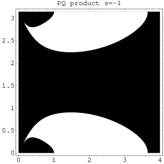
Figure 1:

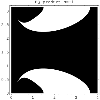
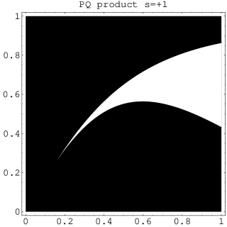
Figure 2:

Figure 3:

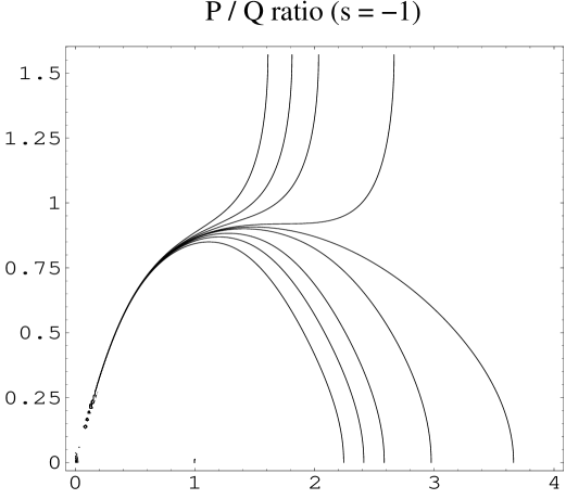
Figure 4:

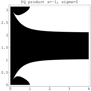
Figure 5:

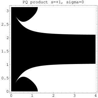
Figure 6:

References

• (1) P. K. Shukla and A. A. Mamun, Introduction to Dusty Plasma Physics (Institute of Physics Publishing Ltd., Bristol, 2002).
• (2) N. N. Rao,   P. K. Shukla and M. Y. Yu,   Planet. Space Sci. 38, 543 (1990).
• (3) P. K. Shukla and V. P. Silin,   Phys. Scr. 45, 508 (1992).
• (4) A. Barkan,   R. Merlino and N. D’Angelo, Phys. Plasmas 2 (10), 3563 (1995).
• (5) J. Pieper and J. Goree, Phys. Rev. Lett. 77, 3137 (1996).
• (6) T. Taniuti and   N. Yajima,   J. Math. Phys. 10, 1369 (1969).
• (7) N. Asano,  T. Taniuti and   N. Yajima,   J. Math. Phys. 10, 2020 (1969).
• (8) M. Remoissenet, Waves Called Solitons (Springer-Verlag, Berlin, 1994).
• (9) P. Sulem, and C. Sulem, Nonlinear Schrödinger Equation (Springer-Verlag, Berlin, 1999).
• (10) A. Hasegawa, Optical Solitons in Fibers (Springer-Verlag, 1989).
• (11) T. Kakutani and N. Sugimoto,   Phys. Fluids 17, 1617 (1974).
• (12) V. Chan and   S. Seshadri,   Phys. Fluids 18, 1294 (1975).
• (13) K. Shimizu and   H. Ichikawa,   J. Phys. Soc. Japan 33, 789 (1972).
• (14) M. Kako,   Prog. Thor. Phys. Suppl. 55, 1974 (1974).
• (15) I. Durrani   et al.,   Phys. Fluids 22, 791 (1979).
• (16) J.-K. Xue,   W.-S. Duan and   L. He,   Chin. Phys. 11, 1184 (2002).
• (17) M. Kako and A. Hasegawa, Phys. Fluids 19, 1967 (1976).
• (18) R. Chhabra   and S. Sharma, Phys. Fluids 29, 128 (1986).
• (19) M. Mishra, R. Chhabra   and S. Sharma, Phys. Plasmas 1, 70 (1994).
• (20) M. R. Amin,   G. E. Morfill   and P. K. Shukla, Phys. Rev. E 58, 6517 (1998).
• (21) W. Duan,   K. Lü and   J. Zhao,   Chin. Phys. Lett. 18, 1088 (2001).
• (22) I. Kourakis and P. K. Shukla, Phys. Plasmas 10 (9), 3459 (2003); ibid, Eur. Phys. J. B, in press (2003).
• (23) Strictly speaking, this result is only true for long wavelengths $\lambda$, compared to the Debye length $\lambda_{D}$ (i.e. small wavenumber $k\ll k_{D}$), as can be readily seen by a numerical analysis of Eq. (39) in Ref. Shimizu ; this is confirmed by Refs. Kakutani and Kako1 . It has been argued that, in principle, the wavenumber threshold $k_{cr}$ for the MI is very high, since ion acoustic modes are physically valid for small $k$, given that Landau damping prevails above a certain value of $k$ kinetic (note that this remark does not concern dusty plasma waves); nevertheless, $k_{cr}$ lowers down once the description is refined - cf. discussion in ref. Chhabra .
• (24) See e.g. Y. H. Ichikawa,   T. Imamura and   T. Taniuti,   J. Phys. Soc. Japan 33, 189 (1972);   H. Sanuki,   K. Shimizu and   J. Todoroki,   J. Phys. Soc. Japan 33, 198 (1972)  Y. H. Ichikawa   and   T. Taniuti,   J. Phys. Soc. Japan 34, 513 (1973).
• (25) M. R. Amin,   G. E. Morfill   and P. K. Shukla, Phys. Plasmas 5 (7), 2578 (1998);   ibid, Phys. Scripta 58, 628 (1998).
• (26) I. Kourakis, Proceedings of the 29th EPS meeting on Controlled Fusion and Plasma Physics, European Conference Abstracts (ECA) Vol. 26B P-4.221 (European Physical Society, Petit-Lancy, Switzerland, 2002); I. Kourakis and P. K. Shukla, Physica Scripta, in press (2003).
• (27) Xue Jukui   and Lang He, Phys. Plasmas 10 (2), 339 (2003).
• (28) A. Mamun   and P. K. Shukla, Phys. Lett. A 290, 173 (2001).
• (29) A. Ivlev   and G. Morfill, Phys. Rev. E 63 (2), 026412 (2001).
• (30) A. A. Mamun   and P. K. Shukla, IEEE Trans. Plasma Sci. 30, 720 (2002).
• (31) Literally speaking, $\alpha$ may take negative values for $\mu>\bigl{(}\frac{\alpha_{2}}{\alpha_{1}}\bigr{)}^{2}=\bigl{(}Z_{i}\,\frac{T_{e}}{T_{i}}\bigr{)}^{2}$, i.e. if $s\frac{Z_{d}\,n_{d,0}}{Z_{i}\,n_{i,0}}>Z_{i}\,\frac{T_{e}}{T_{i}}-1$, indicating a very high concentration of positive dust in the plasma (i.e. assuming ${T_{e}}>{T_{i}}$, this condition can not be fulfilled for $s=-1$); this is, in fact, not a realistic physical situation PSbook .
• (32) See the discussions in Ref. AMS , and definitions therein, according to which both $\alpha$, $\beta$ may be negative in the DIAW case. Also note, for reference, that upon setting: $\alpha=-1/2$, $\alpha^{\prime}=1/6$, $\beta=1$ and $s=1$ in (8), one readily recovers the model equation system for the ion-acoustic waves, e.g. exactly (1) in Ref. chin3 (also Ref. Shimizu for $\sigma=0$).
• (33) Let $k_{1}$ the zero of $P$ i.e. the value of $k$ beyond which $P(k)$ changes sign: $k_{1}=1+\sqrt{4+\frac{3\beta}{\gamma\sigma}}$, taking finite values for $\sigma\neq 0$. This does not contradict the remark made in Ref. chin3 that $P>0$ for $k<1$ (for $\theta=0$ only).
• (34) This remark is in agreement with the ion-acoustic wave case: see Eq. (41) in Ref. Shimizu ); as a matter of fact, the factor $1/3$ therein is also exactly recovered here upon setting the appropriate parameter values (see in Ref. commentdiaw ) into Eq. (46).
• (35) A. Hasegawa, Plasma Instabilities and Nonlinear Effects (Springer-Verlag, Berlin, 1975).
• (36) R. Fedele et al., Phys. Scripta T 98 18 (2002); also, R. Fedele and H. Schamel, Eur. Phys. J. B 27 313 (2002).
• (37) This result is immediately obtained from Ref. Fedele , by transforming the variables therein into our notation as follows: $x\rightarrow\zeta$,   $s\rightarrow\tau$,   $\rho_{m}\rightarrow\rho_{0}$,  $\alpha\rightarrow 2P$,  $q_{0}\rightarrow-2PQ$,  $\Delta\rightarrow L$,  $E\rightarrow\Omega$,  $V_{0}\rightarrow u$.
• (38) R. Tang and J. Xue, Phys. Plasmas 10, 3800 (2003).