Hybrid Particle-Fluid Modeling of Plasmas

Abstract

There are many interesting physical processes which involve the generation of high density plasmas in large volumes. However, when modeling these systems numerically, the large densities and volumes present a significant computational challenge. One technique for modeling plasma physics, the particle in cell (PIC) approach, is very accurate but requires increasing computation time and numerical resolution as the density of the plasma grows. In this paper we present a new technique for mitigating the extreme computational load as the plasma density grows by combining existing PIC methods with a dielectric fluid approach. By using both descriptions in a hybrid particle-fluid model, we now can probe the physics in large volume, high density regions. The hybrid method also provides a smooth transition as the plasma density increases and the ionization fraction grows to values that are well described by the fluid description alone. We present the hybrid technique and demonstrate the validity of the physical model by benchmarking against a simple example with an analytic solution.

1. Introduction

Particle in cell (PIC) methods enjoy great success in modeling devices that include moderately dense plasmas. However, as the plasma density becomes high in a large volume, the number of particles to track becomes computationally prohibitive. Reducing the number of particles by creating larger “macro particles” introduces unacceptable numerical error. Alternatively, high density plasmas in large volumes can be modeled using a dielectric fluid description. This requires integrating over the time dependent distribution function of electrons in the plasma, which for computational simplicity is often assumed to be well approximated by a Maxwellian. However, this is not accurate for characterizing the formation of very dense plasmas, where often times the distribution function is not entirely known. For example, some physical processes such as air breakdown phenomena involve energy distributions that are partially Maxwellian but include a long, high energy tail. The particles in the high energy tail are those responsible for the majority of interactions that lead to a qualitative change in physical behavior Nicholson (Nicholson 1983). Thus, a fluid description that neglects the high energy tail fails to capture the physics of interest. We propose a hybrid plasma description that simultaneously employs the fluid and PIC treatments which has the potential to capture the relevant physics in a tractable computational time.

In addition to reducing the number of particles that must be tracked by the PIC treatment, the particle-fluid hybrid approach also allows computations to be performed on a much coarser grid while preserving the physics. In general, explicit PIC computations become inaccurate when the resolution of the grid becomes comparable to the Debye length of the plasma. In the hybrid scenario, however, the size of the grid need only be comparable to the Debye length of the partial-plasma comprised of the particles in the high energy tail. Since the Debye length varies inversely as the $\sqrt{{\rm density}}$, and the high energy tail contains only a small fraction of the total density, the grid resolution can be significantly reduced. The grid resolution requirements are determined by the Debye length of the partial-plasma and by the length scale required to resolve the spatial gradients in the dielectric fluid treatment. The division criterion used to separate the plasma into particles and fluid will determine which of these conditions will require the greater resolution.

In the hybrid description we use a fluid model for particles that fall within a Maxwellian energy distribution, and PIC for particles in the high energy tail. We have added a dielectric fluid description of a plasma to the Improved Concurrent Electromagnetic Particle In Cell (ICEPIC) code (Birdsall & Langdon (1985); Luginsland & Peterkin (2002)). To ensure physical accuracy the PIC and fluid descriptions are tested independently. A test problem with a simple analytic solution is used to benchmark the performance of the particle, dielectric fluid, and particle-fluid hybrid treatments. All three approaches are shown to properly reproduce the correct dispersion relation when electromagnetic plane waves are launched through a 2-D box containing hot or cold plasma.

2. Method

2.1. The Particle In Cell (PIC) treatment

ICEPIC computes the time advance of the magnetic field according to Faraday’s law, and the electric field according to Ampere-Maxwell’s law. The discreet form of these equations used in ICEPIC are designed to preserve the constraint equations $\nabla\cdot{\bf B}=0$ and $\nabla\cdot{\bf E}=\rho/\epsilon_{0}$ as long as the initial data satisfies these constraints. The particles used in ICEPIC are “macro-particles” that represent many charged particles (electrons and/or ions) with a position vector ${\bf x}$ and a velocity vector ${\bf v}=d{\bf x}/dt$. The relativistic form of Lorentz’s force equation is used to determine the particle’s velocity:

$${\bf F}=m{d\gamma{\bf v}\over dt}=q\left({\bf E}+{{\bf v}\over c}\times{\bf B}\right)$$ (1)

where $\gamma$ is the the usual relativistic factor of $(1-v^{2}/c^{2})^{-1/2}$, and $q$ and $m$ are the charge and mass of the particle.

ICEPIC uses a fixed, Cartesian, logical grid to difference the electric and magnetic field equations. The vector quantities ${\bf E}$, ${\bf B}$, and ${\bf J}$ are staggered in their grid location using the technique of Yee (1966). ${\bf E}$ and ${\bf J}$ are located on the edges of the primary grid, whereas ${\bf B}$ is located on the faces of the primary grid. An explicit leap-frog time step technique is used to advance the electric and magnetic fields forward in time. The advantages of the leap-frog method are simplicity and second-order accuracy. The electric field advances on whole integer time steps whereas the magnetic field and the current density advance on half integer time steps.

The three components of the momentum and position of each particle are updated via Eq. (1) using the Boris relativistic particle push algorithm Boris (Boris 1970). The particle equations for velocity and position are also advanced with a leap-frog technique. The velocity components are advanced on half integer time steps, and the particle positions are updated on integer time steps. The current density weighting employs an exact charge conserving current weighting algorithm by Villasenor & Buneman (1992), enforcing $\nabla\cdot{\bf E}=\rho/\epsilon_{0}$. Once the particles’ positions and velocities are updated and the new current density is updated on the grid, the solution process starts over again by solving the field equations.

2.2. The Dielectric Fluid Model

For very dense plasmas, it is often a very good approximation to treat the plasma as a dielectric fluid. In the presence of EM radiation, this approximation is good for time-scales over which the fluid moves a negligible amount. The dielectric constant used in the fluid approximation is (in terms of the permittivity of free space $\epsilon_{0}$, the collision frequency $\nu_{s}$, and the frequency of the electromagnetic radiation $\omega_{\text{\tiny EM}}$)

$$\epsilon=\epsilon_{0}\left(1-{\omega_{p}^{2}\over\omega_{\text{\tiny EM}}(\omega_{\text{\tiny EM}}+i\nu_{s})}\right)$$ (2)

where the plasma frequency $\omega_{p}$ depends on the density $n_{0}$ and species ($m$, $q$) of the ionized particles, and is given by $\omega_{p}^{2}=n_{0}q^{2}/m\epsilon_{0}$.

To model high density plasma in the time domain, consider Ampere’s law with the plasma dielectric constant;

$$\nabla\times {\bf B}({\bf x},\omega_{\text{\tiny EM}})=$$

$$\mu_{0}\epsilon_{0}\left(-i\omega_{\text{\tiny EM}}+{\omega_{p}^{2}\over\nu_{s}-i\omega_{\text{\tiny EM}}}\right){\bf E}({\bf x},\omega_{EM})$$ (3)

The equivalent expression in the time domain is given by

$$\nabla\times {\bf B}({\bf x},t)=$$

$$\mu_{0}\epsilon_{0}{\partial{\bf E}({\bf x},t)\over\partial t}+\omega_{p}^{2}\mu_{0}\epsilon_{0}\int_{-\infty}^{t}e^{-\nu_{s}(t-\tau)}{\bf E}({\bf x},\tau)d\tau$$ (4)

Differentiating Eq. (4) with respect to time and substituting the result back into Eq. (4) eliminates the convolution integral and yields the following expression used to define the field update equations in the dielectric fluid model.

$${\partial^{2}{\bf E}({\bf x},t)\over\partial t^{2}} +\nu_{s}{\partial{\bf E}({\bf x},t)\over\partial t}+\omega_{p}^{2}{\bf E}({\bf x},t)$$

$$={1\over\mu_{0}\epsilon_{0}}\nabla\times\left({\partial{\bf B}({\bf x},t)\over\partial t}+\nu_{s}{\bf B}({\bf x},t)\right)$$ (5)

Our implementation of this equation, together with Faraday’s law used for updating ${\bf B}$ in our treatment, is displayed in the inset on the following page. It can be shown that this method exhibits 2nd order accuracy, which is demonstrated later in this paper. We have determined that this update is stable if the condition (6) is satisfied:

$$\cos(\omega_{p}\Delta_{t})\leq(X-1)/(X+1)$$ (6)

where

$$X=\frac{4c^{2}}{\omega^{2}}\left(\frac{1}{\Delta_{x}^{2}}+\frac{1}{\Delta_{y}^{2}}+\frac{1}{\Delta_{y}^{2}}\right).$$

The equations used in ICEPIC to perform the ${\bf E}$ and ${\bf B}$ field updates.

${\bf E}^{n+1}=2f_{1}(\Delta_{t},\omega_{p},\nu_{s}){\bf E}^{n}-e^{-\nu_{s}\Delta_{t}}{\bf E}^{n-1}+{1\over\mu_{0}\epsilon_{0}\omega_{p}^{2}\Delta_{t}}\nabla\times\left[\nu_{s}\Delta_{t}\left({\bf B}^{n+1/2}+{\bf B}^{n-1/2}\right)f_{2}(\Delta_{t},\omega_{p},\nu_{s})\right.$

$\left.+2\left({\bf B}^{n+1/2}-{\bf B}^{n-1/2}\right)\left[\left(1-{\nu_{s}^{2}\over\omega_{p}^{2}}\right)f_{2}(\Delta_{t},\omega_{p},\nu_{s})+\nu_{s}\Delta_{t}e^{-\nu_{s}\Delta_{t}/2}\;{\rm sinh}\left(\nu_{s}\Delta_{t}/2\right)\right]\right]$

${\bf B}^{n+1/2}={\bf B}^{n-1/2}-\Delta_{t}\nabla\times{\bf E}^{n}$

where

$f_{1}(\Delta_{t},\omega_{p},\nu_{s})=e^{-\nu_{s}\Delta_{t}/2}\;{\rm cosh}\left({\Delta_{t}\over 2}\sqrt{\nu_{s}^{2}-4\omega_{p}^{2}}\right)$

$f_{2}(\Delta_{t},\omega_{p},\nu_{s})=e^{-\nu_{s}\Delta_{t}/2}\left({\rm cosh}\left(\nu_{s}\Delta_{t}/2\right)-{\rm cosh}\left({\Delta_{t}\over 2}\sqrt{\nu_{s}^{2}-4\omega_{p}^{2}}\right)\right)$

2.3. Numerical Methods to Create Hybrid Models

Developing a consistent way to divide the simulated plasma into fluid and particle portions is one of the more complicated aspects of this approach. Several details need to be considered. Most importantly, the distinction between the fluid and particle descriptions is not a physical one, but rather a computational necessity. As such, it is crucial that dividing the plasma into two separate populations does not introduce any spurious observable behaviors in the physics. The real-world plasma is not divided, so the particles and the fluid must be compelled to interact as a single species. This manifests itself in two ways; first, the mechanism for exchanging particles into fluid (and vice versa) must be seamless enough that it does not affect the global properties of the plasma. Second, the fluctuations in density, pressure, and temperature in the fluid must affect the dynamics of the PIC particles in exactly the same way as if those fluctuations had occurred in a purely PIC model. In the special case where the density contained in the fluid is significantly greater than the density in the particles, it may be a good approximation to neglect these fluctuations in the PIC particles. This is discussed later in section 2.5.

Another important priority in the development of a useful hybrid model is to determine the optimal way to divide the plasma. An appropriate criterion must be found for the exchange of PIC particles with fluid density. It is important to treat as much of the plasma as possible with the fluid model, since this minimizes computation time. On the other hand, if the decision criterion is computationally expensive, it would not be sensible to perform the particle-fluid exchange in every time step. A balance must be found between the time saved by moving particles into the fluid and the time spent deciding whether the particles can be moved without sabotaging the accuracy of the simulation.

Finally, although collision physics have been added to the fluid and PIC models independently, collisions between particles and elements of fluid have not yet been modeled and tested for the current simulations, and are a subject for future study. Ultimately, these will affect the balance of the energy and the density in the fluid. More extensive future modeling will include the effects of mobility, diffusion, ionization with the background gas, and feedback heating from the external fields.

2.4. Discussion of Hybrid Errors and Limitations

Quantitatively, implementing a hybrid approach is accomplished by dividing the distribution of the plasma $f$ into two separate populations, $f_{1}$ and $f_{2}$. The distributions $f_{1}$ and $f_{2}$ sum to the total distribution $f=f_{1}+f_{2}$ and for simplicity are positive definite such that $f_{1}<f$ and $f_{2}<f$. From a fluid perspective, the continuity equation and fluid force equations are obtained by taking the first two moments of the Vlasov equation, which dictates the evolution of the plasma distribution function in a 6+1 dimensional (${\bf x}$,${\bf v}$,$t$) phase space.

$$\partial_{t}f({\bf x},{\bf v},t)+{\bf v}\cdot\nabla_{x}f+{q\over m}\left({\bf E}+{{\bf v}\over c}\times{\bf B}\right)\cdot\nabla_{v}f=0$$ (7)

Here the effects of collisions are ignored. Since each term in the Vlasov equation is linear in $f$, the continuity and force equations contain no terms proportional to $f_{1}f_{2}$, and can be satisfied by evolving the two populations separately. For the test problem presented in the following section, one of the two populations is evolved using the PIC technique, while the other population is treated as a dielectric fluid. The PIC technique automatically satisfies the continuity and force equations, but our implementation of the dielectric fluid does not contain two of the terms in the force equation; the $(q/mc)n({\bf v}\times{\bf B})$ term and the $\nabla_{x}\cdot(n\langle{\bf vv}\rangle)$ term. The justification for neglecting these terms is that drift velocities in the fluid will be small, and components of the plasma with high energies and velocities will be modeled with PIC particles.

When collisions are added the description becomes more complex because collisions will have to be modeled between populations, as well as within each population. In this case linearity is lost, and it may not be possible to decouple the evolution of the two populations. It may, however, be acceptable to make certain simplifying assumptions, such as $n_{{\rm particles}}<<n_{{\rm fluid}}$. In this limit, the contribution to the fluid dynamics from fluid-fluid collisions far exceed the contribution from fluid-particle collisions, and the latter might safely be neglected. The error introduced by this assumption will depend on the relative distributions $f_{1}$ and $f_{2}$. When implementing the model of collisions it is necessary to estimate analytically the error introduced as a function of the particle density $n_{{\rm particles}}$, and re-distribute the populations when a pre-determined threshold for error is reached. The error analysis of this method to incorporate collisions into the hybrid plasma model is currently under investigation.

2.5. The Dispersion Relation

To demonstrate that the numerical methods discussed above are valid treatments of high density plasma physics in large volumes, we have employed these methods to calculate the dispersion relation of electromagnetic plane waves traveling through a plasma in a two dimensional box. This is simple enough that an analytic expression for the dispersion relation exists, and also small enough to make an explicit PIC treatment practical, even for very high densities. In this way we are able to directly compare the theoretical prediction of the dispersion relation to the results of the individual particle (PIC) and dielectric fluid treatments, and to the PIC-fluid hybrid computation. We perform all the calculations (analytic and numerical) in the limit of non-relativistic thermal velocities in the plasma, a good approximation in clouds of plasma recently ionized by directed energy sources.

The analytic expression relating the frequency $\omega_{\text{\tiny EM}}$ of transverse electromagnetic waves to the wave number $k$ in a cold plasma is given by the following dispersion relation (see e.g. Chen (1984)):

$$\omega_{\text{\tiny EM}}^{2}=\omega_{p}^{2}+k^{2}c^{2}\;\;\;.$$ (8)

Here the plasma frequency $\omega_{p}$ depends on the density and and species of the plasma and is given in section 2.2. and the collision frequency $\nu_{s}$ is assumed to be zero. The expression for the dispersion relation becomes significantly more complicated for a warm plasma, because thermal velocities allow for a coupling between adjacent regions in the equations of motion, due to local pressure gradients. However, in the non-relativistic limits being considered here, the change in the dispersion relation due to thermal fluctuations is less than 0.01%, and we neglect the effect.

We have performed simulations in a simple geometry in order to extract the numerical dispersion relation and compare the results to the theoretically expected curve. A row of dipole antennas polarized in the $\hat{z}$ direction are lined up at the left end of a long box filled with a relatively dense cold plasma ($1.43\times 10^{17}\text{electrons}/m^{3}$ corresponding to a plasma frequency of $\omega_{p}=21.1\times 10^{9}$ rad/sec). The antennas are driven in phase with an oscillating current, at a peak amplitude of $0.1$ Amps, to generate a plane wave in the plasma. The top and bottom edges of the box are defined by metal boundaries. There is a perfectly matched layer (PML) on both the left and right sides of the box to prevent any reflection of incoming EM waves, simulating an infinite domain in that direction. A cartoon of the geometry is shown in Figure (1). Simulations run from one to four light crossing times. At one light crossing time there are observable transient effects while the current in the antennas ramps up, while at 4 light crossing times there is significant beating from reflections off of the interior of the plasma. While these effects make it difficult to quantify properties of the plasma such as the skin depth or transmission and reflection coefficients, neither of them affected the calculated values of $k$ associated with the frequency of the incoming plane wave.

Figure 1.— A 2-D box with metal on top and bottom, PML on left and right, and a cold plasma in the interior. The line of dipole antennas (polarized in $\hat{z}$) generating the EM plane wave is marked with dots on the left side. The dimensions of the box are $1.4m\times 0.5m$

To bench-mark the performance of the PIC-fluid hybrid treatment, we first run simulations in this geometry with the plasma consisting of only PIC particles, then with only dielectric fluid. We then test a model where half of the plasma is treated as PIC particles and the other half modeled as a fluid. This division is in each cell, rather than in different spatial regions in the box. There is no mechanism for exchange between fluid and particles. The simulations are run using many frequencies of the EM plane waves, thus providing several different data points to fit to the theoretical dispersion curve. To calculate the value of $k$, the pixels are averaged in the $\hat{y}$ direction, and a spatial Fourier transform taken of the resulting 1-D ($\hat{x}$) array. The error in the resulting wave number $k$ is inherited from the finite box size.

3. Results

The dispersion relations obtained from the explicit PIC, dielectric fluid, and fluid-PIC hybrid models are displayed in Figure (2) along with the theoretical value from Eq. (7). Although the value of k is the dependent variable in our analysis, we plot the wavenumber on the x axis so the dispersion relation takes its familiar form. All three modeling techniques yield the same values of k within the resolution of the simulations; they agree to within $\pm 2.5$ cycles/$m$, approximately the width of the symbols used in the plot.

Figure 2.— The dispersion relation for E-M plane waves traveling through a cold plasma in a 2-D box. This plot shows simultaneously the results for the PIC, dielectric fluid, and PIC-fluid hybrid models. All three models yielded results that fell in the same bin in k with an error bar of $\pm 2.5$ cycles/$m$, and are labeled ICEPIC in the plot.

The transmission of electromagnetic radiation through a plasma as a function of the plasma density and chemical properties is another interesting quantity to consider when evaluating the validity of the particle-fluid hybrid model. We are particularly interested in probing the regime where the frequency of the electromagnetic radiation is comparable to the plasma frequency. To calculate the transmission coefficient as a function of the frequency of the plane wave, we modified the geometry of the previous simulation to include three regions; a vacuum region containing the antennas, a region in the center containing a cold plasma with the same density, and a third vacuum region on the right. The amplitudes are calculated by taking the Fourier transform of the time history of the quantity $({\bf E}-c{\bf B})/2$, which represents the magnitude of the right-going electromagnetic wave in a vacuum. The ratio of the amplitudes in the two vacuum regions is plotted as a function of frequency in Figure (3).

Figure 3.— The fraction of a plane wave transmitted through a $7cm$ region of plasma of density $1.43\times 10^{17}$ electrons/$m^{3}$.

The theoretical curve in Figure (3) is obtained from the boundary matching at the two vacuum-plasma interfaces. The positions of the maxima and minima in the transmission coefficient depend upon the width of the plasma region, in this simulation $7cm$.

Although there is striking agreement between the computed values of the transmission coefficients and dispersion relation with the theoretically predicted curves, a formal demonstration of the convergence of the code is needed to be sure that the resolution is sufficient to accurately model the physics. We have examined the transmission at three different wavelengths of incident radiation, corresponding to a local maximum ($\lambda=7.0$ cm), a local minimum ($\lambda=7.73$ cm), and an area of high slope nearer to the plasma frequency($\lambda=8.25$ cm). For each of these cases, the spatial resolution of the grid was varied from 6 to 40 cells per free-space wavelength of the incident radiation. When there were particles in the simulations, the total number of particles was kept fixed. At the finest spatial resolution there were enough particles per cell to maintain numerical accuracy. The results of this investigation are summarized in Figure (4), which demonstrates 2nd order convergence to the theoretical value. From Figure (4) we conclude that at a resolution of 20 cells per wavelength, the resolution used when generating Figures (2)and (3), the code has converged to produce less than 6% worst-case error from the theoretical value. Seven of nine runs at this resolution produced errors less than 1%. Simulations yielding errors larger than 1% correspond to a wavelength of 8.25 cm, which is in a high slope region of the theoretical curve. Here, the small errors in plasma width as represented by the grid lead to larger errors in the simulated transmission. The reader should be reminded that differences between the computed and theoretical values have contributions from error in the modeling, approximations in the calculation of the theoretical value, and numerical errors due to finite resolution.

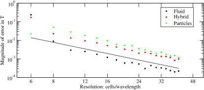
(a) $\lambda_{\rm vac}=7cm$

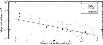
(b) $\lambda_{\rm vac}=7.73cm$

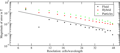
(c) $\lambda_{\rm vac}=8.25cm$

Figure 4.— Error in the transmission coefficient, T, as a function of grid resolution for fluid, particle, and particle-fluid hybrid models, evaluated at three different incident wavelengths. The solid lines show the slope of 2nd order convergence.

4. Conclusions

We demonstrate the validity of a powerful new technique that allows numerical simulations of high density plasmas in large volumes to be computationally tractable in reasonable times. Among other applications such as tokamaks, plasma processing, atmospheric plasmas (lightning, red sprites, blue jets), plasma-display plasmas, and lighting, this approach will aid in the exploration of many unanswered questions about Radio Frequency (RF) breakdown in air. We are particularly interested in understanding the mechanisms of breakdown. High density plasmas in large volumes occur relatively frequently when studying High Power Microwave (HPM) or other directed energy devices. Sources of high power microwaves can cause RF breakdown in air or other gaseous media in the vicinity of the antenna. It is extremely useful for design exploration if such breakdown processes could be modeled computationally. Several details can be added to make this tool even more useful. Collisional interactions can be implemented in both the PIC and fluid treatments, taking care that collisional interactions between the populations are accurately modeled. The treatment should also be adapted to accommodate relativistic particle velocities. Reasonable mechanisms need to be added for interchange of particles to fluid, and vice versa. These mechanisms must be treated with care so as not to introduce any spurious effects into the physics.

When collisions and gas chemistry have been fully implemented we will use this method to explore the details of the plasma formation as a function of the pulse width, the ${\bf E}$ field intensities causing the breakdown, and the properties of the background gas (density, impurities). We hope to quantitatively determine when the breakdown occurs and what fraction of the RF pulse is reflected, an effect that causes tail erosion. By determining the ionization states that are produced, and the densities that are reached, we will be able to describe how the global properties of the medium will change.

The authors would like to thank Matthew Bettencourt, Peter J. Turchi and Kyle Hendricks for useful discussions on this work. This research was supported in part by Air Force Office of Scientific Research (AFOSR).

References

- Birdsall & Langdon (1985) Birdsall, C.K., Langdon, A.B., Plasma Physics Via Computer Simulation, McGraw-Hill, New York, (1985)
- (2) Boris, J.P., “Relativistic Plasma Simulation-Optimization of a Hybrid Code,” Num. Sim. Plasmas, Navan Res. Lab., Wash D.C., (1970) pp3-67
- Chen (1984) Chen, F.F., Introduction to Plasma Physics and Controlled Fusion Volume 1, Plenum Press, New York, (1984)
- Luginsland & Peterkin (2002) Luginsland, J.W., Peterkin, R.E., “A Virtual Prototyping Environment for Directed Energy Concepts,” Computing in Science & Engineering; March-April (2002); vol.4, no.2, pp.42-9
- (5) Nicholson, Dwight R., Introduction to Plasma Theory, Krieger Publishing Company, (1983)
- Villasenor & Buneman (1992) Villasenor, J., Buneman, O., “Rigorous Charge Conservation for Local Electromagnetic Field Solvers,” Comp. Phys. Comm, 69 306 (1992)
- Yee (1966) Yee, K.S., “Numerical Solution of Initial Boundary Value Problems Involving Maxwell’s Equations in Isotropic Media,” IEEE Trans. Ant. Prop., AP-14 (1966) 302