On the possibility of “correlation cooling” of ultracold neutral plasmas

Abstract

Recent experiments with ultracold neutral plasmas show an intrinsic heating effect based on the development of spatial correlations. We investigate whether this effect can be reversed, so that imposing strong spatial correlations could in fact lead to cooling of the ions. We find that cooling is indeed possible. It requires, however, a very precise preparation of the initial state. Quantum mechanical zero-point motion sets a lower limit for ion cooling.

Experimentally, ultracold ($T\ll 1$ K) neutral plasmas could be realized only recently by photoionizing a cloud of ultracold atoms [1, 2, 3]. From a plasma physics perspective, they are very appealing since they might provide laboratory realizations of so-called strongly coupled plasmas, where the Coulomb interaction (inversely proportional to the mean inter-particle spacing $a$) dominates the random thermal motion (proportional to the temperature $T$). As a consequence, interesting ordering phenomena such as Coulomb crystallization can be observed. In order to be in this strong-coupling regime, a system has to be either very dense (large Coulomb interaction) or very cold (little thermal energy). The first scenario is realized in some astrophysical contexts, which are difficult to access experimentally. Hence, the possibility to realize a strongly coupled plasma in the laboratory by going to ultralow temperatures offered exciting prospects within the plasma physics community. In [1], an ultracold neutral plasma has been created by photoionizing a gas of laser-cooled Xe atoms. The extremely low temperatures of the Xe gas suggested that the system was well within the strong-coupling regime, the so-called Coulomb coupling parameter $\Gamma\equiv e^{2}/(ak_{\rm B}T)$, i.e. the ratio of potential to thermal energy, being of the order of $10$ for the electrons and even up to $30000$ for the ions.

However, it was realized quickly [4, 5, 6] that despite the low temperature of the Xe gas a strongly coupled plasma could not be created in this way. Due to the fact that the neutral Xe atoms initially present interact only very weakly, the plasma is created in a completely uncorrelated non-equilibrium state. Hence, the subsequent conversion of potential into kinetic energy rapidly heats both the electron and ion subsystem, suppressing the development of substantial correlations [4, 7]. This effect has been termed “disorder-induced heating” [6] or “correlation-induced heating” [8], expressing the fact that it is the development of spatial correlations during the relaxation of the plasma towards an equilibrium state which leads to an increase in temperature. Put another way, in the initial non-equilibrium state the potential energy is higher than in the corresponding equilibrium state of a plasma of the same average density. Consequently, relaxation towards thermodynamic equilibrium will reduce the potential energy in the system and increase the kinetic energy, i.e. the temperature. Additionally, the electrons are heated by three-body recombination as well as continuum lowering. Suppression of electron heating is thus much more difficult than simply reducing the correlation heating. At present, there is a proposal of mixing the plasma with a gas of Rydberg atoms, so that collisional ionization of these Rydberg atoms removes energy from the electron component of the plasma [9].

For the creation of a strongly coupled ionic component, different procedures have been suggested to avoid these heating effects, namely (i) using fermionic atoms cooled below the Fermi temperature in the initial state, so that the Fermi hole around each atom prevents the occurence of small interatomic distances [7]; (ii) an intermediate step of exciting atoms into high Rydberg states, so that the interatomic spacing is at least twice the radius of the corresponding Rydberg state [6]; and (iii) the continuous laser-cooling of the plasma ions after their initial creation, so that the correlation heating is counterbalanced by the external cooling [10, 11]. So far, none of these procedures has been realized experimentally, however it has been shown theoretically that continuous laser-cooling can indeed lead to a strongly coupled plasma, connected with crystallization of the expanding system [11]. In this case, the correlation heating effect is still present and is offset by an additional external cooling mechanism. Proposals (i) and (ii), on the other hand, aim at suppressing the heating directly by avoiding the small interparticle distances leading to a large potential energy, i.e. by introducing (spatial) correlation in the initial state. As has already been noted in [6], this could also be achieved using optical lattices to arrange the atoms.

At this point, the question arises naturally whether the correlation heating could not only be avoided, but whether it can actually be reversed and turned into cooling. As argued above, correlation heating describes the fact that the uncorrelated ions created in the photoionization process have a higher potential energy than in the thermodynamical equilibrium state. Hence, equilibration will reduce the potential energy and increase the kinetic energy of the system, making the ions hotter than the atoms in the initial gas state. On the other hand, it is conceivable that the atomic gas might be prepared in an “overcorrelated” state, where the potential energy is lower than its equilibrium value. In this case, equilibration must increase the potential energy on the cost of the kinetic energy, i.e. the temperature must decrease. This effect of “correlation cooling” has been described before in [12] and, based on a kinetic approach, in more general terms in [13]. In [12], the overcorrelated initial state was achieved by suddenly decreasing the Debye screening length, i.e. the temperature of the electrons, rather than by inducing spatial order. It was shown that in this way, a reduction in temperature of the order of a few percent does indeed occur for the temperatures and densities considered.

In the present letter, we explore an alternative scheme for achieving correlation cooling, namely the use of an optical lattice to induce spatial correlations in the initial state as suggested in [6]. We describe, both analytically and by molecular dynamics simulations, the situation of a fully ordered initial state where the atoms have been arranged in a perfect bcc-type lattice structure using an optical lattice. In reality, their spatial distribution will be broadened, classically due to their non-vanishing kinetic energy corresponding to the initial-state temperature, quantum mechanically corresponding to the eigenstates of the harmonic oscillator potential generated by the optical lattice. This broadening is neglected in our numerical simulations, however, its influence will be discussed in the analytical considerations below. For the sake of numerical simplicity, our initial state corresponds to a sphere cut out from a bcc lattice rather than a more realistic cylindrical shape, arguing that edge effects should be of minor importance if the number of atoms in the system is large enough. The system is propagated using the hybrid molecular dynamics method described in [11]. Briefly, an adiabatic approximation is employed for the electrons, and their distribution is obtained from the steady-state King distribution [14], widely used in the study of globular clusters. The ions are then propagated using the electronic mean-field obtained from the steady-state distribution and by fully taking into account the ion-ion interactions. In the experiments under consideration, quasineutral plasmas with $\Gamma_{\rm{e}}$ as low as $4\cdot 10^{-3}$ [2] have been realized, making Debye screening effects negligible, while ion numbers $N_{\rm i}$ up to $10^{8}$ have been obtained [15]. For our simulations, such a large particle number would lead to a prohibitively large numerical effort. However, the typical timescale for the plasma expansion is $t_{\rm exp}\approx\sqrt{\Gamma_{\rm e}}N_{\rm i}^{1/3}\omega_{0}^{-1}$, where $\omega_{0}=\sqrt{e^{2}/Ma^{3}}$ is the Einstein frequency in the Wigner-Seitz model of a Coulomb solid and $M$ is the ion mass. On the other hand, the relaxation of the ions takes place on a timescale of $t_{\rm rel}\approx\omega_{0}^{-1}$. Hence, the same macroscopic behavior can be obtained by decreasing $N_{\rm i}$ and increasing $\Gamma_{\rm{e}}$, keeping the ratio $t_{\rm exp}/t_{\rm rel}$ fixed. Therefore, for our simulations we chose $N_{\rm i}=10^{5}$ and an initial electron energy corresponding to $\Gamma_{\rm{e}}=0.5$, while the bare Coulomb potential was used for the ion-ion interaction.

Figure 1(a) shows the time evolution of the average ion kinetic energy in units of the initial-state temperature for a typical realization. Since the initial lattice configuration produces an effective oscillator potential for each ion, the relaxation process is connected with transient oscillations of the kinetic energy which are damped out due to ion-ion collisions. Additionally, the average kinetic energy increases at later times due to a radial ion acceleration caused by the thermal electron pressure, which is proportional to the density gradient. Therefore the slow expansion of the unconfined plasma leads to a softening of the initially sharp plasma edge and a modification of the velocity distribution in the outer region of the plasma only. Since this distribution is close to a Maxwellian in the central region of the plasma, the average kinetic energy is directly related to the ionic temperature $T$, while it becomes more and more dominated by the expansion energy towards the edge of the plasma. In order to highlight these edge effects, we have calculated the average ion kinetic energy from the velocity distribution in the inner region only, taken to be a sphere with half of the initial plasma radius. The resulting curve is shown as the dashed line in figure 1(a). Clearly, the expansion hardly affects the kinetic energy in the inner region of the plasma, leaving only the oscillations which are damped out as the system approaches thermodynamic equilibrium. As discussed above, the relaxation of the ions towards equilibrium takes place on a timescale of $\omega_{0}^{-1}$, while the typical timescale for the plasma expansion is $\sqrt{\Gamma_{\rm e}}N_{\rm i}^{1/3}\omega_{0}^{-1}$. Hence, a sufficiently large number of ions allows for an almost unperturbed relaxation in the inner plasma region so that a temperature can be defined in a meaningful way. (For a strontium plasma with a typical density of $5\cdot 10^{9}$cm${}^{-}3$ used, e.g., in [15], $\omega_{0}^{-1}\approx 0.2\>\mu$s, while $t_{\rm exp}$ is about $30$ times larger for $\Gamma_{e}=4\cdot 10^{-3}$ and $N_{i}=10^{8}$.) Using the absorption imaging techniques described in [15] it should be possible experimentally to probe this inner region only. Therefore, we chose to define the final temperature as given by the inner plasma region and to neglect the finite-size effects associated with the boundary region of the plasma. The resulting $T_{\rm f}$ was estimated from the center of the remaining oscillations and is shown in figure 1(b) as a function of $\Gamma_{\rm i}$ by the full circles. It should be noted that the value of $\Gamma_{\rm i}$ has no meaning as a measure of nonideality of the initial plasma state, since the system may be far from equilibrium. Therefore, in the present case it should simply be viewed as a density-scaled inverse temperature rather than a Coulomb coupling parameter. As can be seen in the figure, the ratio of final to initial temperature reaches a constant value of about 0.5 as the initial temperature goes to zero. Hence, cooling can indeed be achieved on a moderate level of a temperature reduction of about 50 percent.

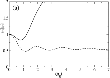
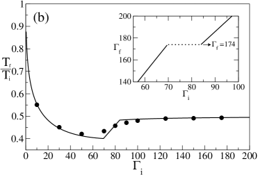
Figure 1: (a) Time evolution of the ionic kinetic energy, for the whole plasma cloud (solid) and for the central region only (dashed). (b) Ratio of final to initial temperature as a function of the density-scaled inverse initial ion temperature $\Gamma_{\rm i}$, from the numerical simulations (full circles) and from equation (6) (solid line). The inset shows the final Coulomb coupling parameter.

For large particle numbers and if $\Gamma_{\rm e}$ is small enough such that three-body recombination and Debye screening can be neglected, quasineutrality leads to a homogeneous electron background in the central plasma region. Thus, we can use the one-component plasma model to gain more insight into the cooling process. This model has been studied extensively over the last decades [16, 17], which led to a detailed understanding of the equation of state over a wide parameter range. In the classical regime, the energy per particle of the final equilibrium state is given by

$$U_{\rm f}=\frac{3}{2}k_{\rm B}T_{\rm f}+W_{\rm f}\equiv(\frac{3}{2}+w_{\rm f})k_{\rm B}T_{\rm f}\;,$$ (1)

where the excess energy $W$ accounts for nonideal effects due to the inter-particle Coulomb interaction. For this quantity, several fit formulae can be found in the literature, which have been obtained by Monte Carlo and molecular dynamics methods [16, 17, 18]. In the fluid phase we use the interpolation formula from [19]

$$w^{\rm fl}(\Gamma_{\rm f})=\Gamma_{\rm f}^{3/2}\left(\frac{A_{1}}{\sqrt{A_{2}+\Gamma_{\rm f}}}+\frac{A_{3}}{1+\Gamma_{\rm f}}\right)\;,$$ (2)

where $A_{1}=-0.9052$, $A_{2}=0.6322$ and $A_{3}=-\sqrt{3}/2-A_{1}/\sqrt{A_{2}}$. Equation (2) satisfies the known small-$\Gamma$ limit [20] and accurately fits the high-$\Gamma$ values obtained by numerical calculations [18]. In the solid phase ($\Gamma>174$), the excess energy can be described by an expansion in powers of $1/\Gamma$ [17]

$$w^{\rm s}(\Gamma_{\rm f})=-A_{\rm m}\Gamma_{\rm f}+\frac{3}{2}+\frac{a}{\Gamma_{\rm f}}+\frac{b}{\Gamma_{\rm f}^{2}}+\frac{c}{\Gamma_{\rm f}^{3}}+{\cal{O}}\left(\frac{1}{\Gamma_{\rm f}^{4}}\right)\;,$$ (3)

where $a=10.84$, $b=352.8$ and $c=1.794\cdot 10^{5}$. Here, the first term corresponds to the Madelung energy of the lattice, with $A_{\rm m}=0.895929$ for a bcc-type lattice. The second term describes thermal contributions corresponding to an ideal gas of phonons while the higher-order terms account for anharmonic corrections. Assuming an unchanged ionic phase-space distribution function directly after the photoionization, where the spatial distribution due to the finite temperature is represented by Gaussian profiles centered on the sites of the bcc lattice, the internal energy of the initial nonequilibrium state is given by

$$U_{\rm i}=\frac{3}{2}k_{\rm B}T_{\rm i}+W_{\rm i}=\frac{3}{2}k_{\rm B}T_{\rm i}-k_{\rm B}T_{\rm i}A_{\rm m}\Gamma_{\rm i}+k_{\rm B}T_{\rm i}\frac{\Gamma_{\rm i}}{2}\left[\frac{\left<r^{2}\right>}{a^{2}}-\frac{7}{8}B\left(\frac{\left<r^{2}\right>}{a^{2}}\right)^{2}\right]\;,$$ (4)

where $B=\frac{1}{2}\sum_{i,j}\frac{a^{5}}{r^{5}_{ij}}$, with $B=0.876719$ for a bcc lattice. While the first two terms correspond to the ion kinetic energy and the Madelung energy of a bcc lattice of point charges, the last two terms give the leading-order corrections due to a broadened charge distribution at the lattice sites expanded in terms of the mean-squared ion displacement $\left<r^{2}\right>$. Assuming an initially non-interacting atomic gas and harmonic trapping potentials we have

$$\frac{\left<r^{2}\right>}{a^{2}}=\frac{3k_{\rm B}T_{\rm i}}{M\omega_{\rm L}^{2}a^{2}}=3\frac{\omega_{0}^{2}}{\omega_{\rm L}^{2}}\Gamma_{\rm i}^{-1}\;,$$ (5)

where $\omega_{\rm L}$ is the oscillation frequency of the trapping potentials. The final temperature is now simply obtained from energy conservation

$$\frac{T_{\rm f}}{T_{\rm i}}=\frac{3/2+w_{\rm i}(\Gamma_{\rm i})}{3/2+w_{\rm f}(\Gamma_{\rm f})}\;,$$ (6)

with $w=w^{\rm fl}$ for $\Gamma\leq 174$ and $w=w^{\rm s}$ for $\Gamma>174$. Figure 1(b) shows the ratio $T_{\rm f}/T_{\rm i}$ as a function of $\Gamma_{\rm i}$ for $\left<r^{2}\right>/a^{2}=0$, i.e. for a point-like ionic density at the lattice sites. A comparison with our numerical data shows that equation (6) reproduces the numerical values for a finite-size plasma quite well. The remaining discrepancies should be attributable to finite-size effects [21, 22]. At small values of $\Gamma_{\rm i}$ the temperature ratio starts out from unity and decreases with increasing $\Gamma_{\rm i}$, since the excess potential energy of the final fluid state is naturally larger than that of the initial lattice configuration. As $\Gamma_{\rm i}$ exceeds a value of $\Gamma_{\rm i}\approx 70$ the temperature ratio rises linearly, connected with a solidification of the plasma, where $\Gamma_{\rm f}=174$ stays constant (see inset). In this regime, regions of fluid and solid phases coexist in the plasma. At $\Gamma_{\rm i}\approx 84$ the system has crossed the melting point and the temperature ratio approaches a value of $1/2$. This factor of $1/2$ originates from the additional thermal energy of $3k_{\rm B}T_{\rm f}/2$ arising from thermal lattice excitations. However, the situation changes if a finite extension of the initial charge distribution at the lattice sites is considered. Neglecting terms of order $\left(\left<r^{2}\right>/a^{2}\right)^{2}$ in equation (4), one finds that for finite $\omega_{\rm L}$ the temperature approaches a value of $(1+\omega_{0}^{2}/\omega_{\rm L}^{2})/2$ if $\left<r^{2}\right>\ll a^{2}$.

Let us now turn to the question of the influence of possible lattice defects, i.e. how perfect must the initial-state lattice be in order to observe correlation cooling? Such defects are easily accounted for in the previous consideration. Introducing a filling factor $f$, defined as the probability that a given lattice site is occupied, simply reduces the average charge at each lattice site. Therefore, the potential energy of the initial state can be written as $f^{2}w_{\rm i}(\Gamma_{\rm i}^{\star})k_{\rm B}T_{\rm i}$, where $\Gamma_{\rm i}^{\star}$ corresponds to the temperature scaled by the density of the perfectly filled lattice, which is related to the actual value of $\Gamma_{\rm i}$ by $\Gamma_{\rm i}^{\star}=f^{-1/3}\Gamma_{\rm i}$. Substituting this in equation (4) yields

$$\frac{T_{\rm f}}{T_{\rm i}}=\frac{3/2+f^{2}w_{\rm i}(f^{-1/3}\Gamma_{\rm i})}{3/2+w_{\rm f}(\Gamma_{\rm f})}$$ (7)

as the generalization of equation (6) to non-perfect filling. In figure 2(a), we show the resulting final temperature as a function

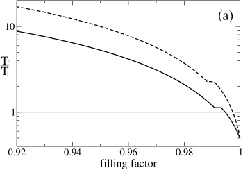
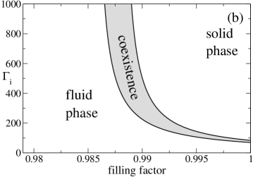
Figure 2: (a) Final temperature as a function of the lattice filling factor for $\Gamma_{\rm i}=200$ (solid line) and $\Gamma_{\rm i}=400$ (dashed line). The gray horizontal line separates cooling from heating. (b) Phase diagram for the final plasma state in the $f$-$\Gamma_{\rm i}$ plane.

of the filling factor for two different $\Gamma_{\rm i}$. A decreasing filling enhances the initial potential energy (compared to that of a full lattice with the same average density, not the same lattice constant), leading to a rapid increase of the final temperature. As a consequence, cooling can be achieved for a nearly perfect lattice only. Furthermore, for a fixed $f<1$, increasing $\Gamma_{\rm i}$ leads to larger values for the temperature ratio. This heating also influences the possibility of the creation of a crystallized plasma phase, since the melting point of $\Gamma_{\rm f}=174$ is shifted to larger values of $\Gamma_{\rm i}$, as shown in the phase diagram figure 2(b). For values of $f<0.9855$, the system always ends up in the fluid phase independent of $\Gamma_{\rm i}$.

The above picture suggests that, for a perfect initial state, cooling is always possible independent of the initial temperature. At low enough temperatures, however, the classical treatment will break down, and quantum mechanical effects will become important. As in the classical case the quantum statistical internal energy of a Coulomb solid can be written as a sum of the Madelung energy, harmonic contributions arising from linear lattice excitations and anharmonic corrections. For the harmonic contributions to the excess energy we use an analytic approximation formula obtained recently [23], which reproduces the numerical results for harmonic Coulomb crystals very accurately. The anharmonic corrections are taken from [24], where they were obtained by fitting the results of quantum Monte Carlo simulations. The resulting expression is too lengthy to be reproduced here, but incorporates both the known semiclassical high-temperature limit as well as the quantum mechanical groundstate energy of a Coulomb crystal,

$$w_{\rm gs}=-A_{\rm m}\Gamma_{\rm f}+1.329\theta-\frac{0.365}{\sqrt{r_{\rm s}}}\theta+{\cal{O}}\left(\frac{\theta}{r_{\rm s}^{3/2}}\right)\;.$$ (8)

Here, $\theta=(\hbar\omega_{0})/(k_{\rm B}T)$ measures the importance of quantum effects, i.e. zero-point ion oscillations, and $r_{\rm s}=aMe^{2}/\hbar^{2}$ is the Wigner-Seitz radius in units of the ionic Bohr radius. As in the previous classical considerations, we apply a sudden approximation assuming an unchanged density matrix directly after the photoionization pulse. The initial energy of the plasma is thus found from the expectation value of the new Hamiltonian using a density matrix representing independent harmonic oscillators arranged on a bcc lattice. The result is

$$U_{\rm i}=\frac{3}{4}\hbar\omega_{\rm L}\coth{\left(\frac{\hbar\omega_{\rm L}}{2k_{\rm B}T_{\rm i}}\right)}-k_{\rm B}T_{\rm i}A_{\rm m}\Gamma_{\rm i}+k_{\rm B}T_{\rm i}\frac{\Gamma_{\rm i}}{2}\left[\frac{\left<r^{2}\right>}{a^{2}}-\frac{7}{8}B\left(\frac{\left<r^{2}\right>}{a^{2}}\right)^{2}\right]\;,$$ (9)

which exactly corresponds to the classical expression equation (4) except that the kinetic energy $3k_{\rm B}T_{\rm i}/2$ is replaced by its quantum mechanical counterpart. Moreover, the mean-squared displacement is now given by

$$\frac{\left<r^{2}\right>}{a^{2}}=\frac{3}{2}\nu\;{\rm{coth}}\left(\frac{\hbar\omega_{\rm L}}{2k_{\rm B}T_{\rm i}}\right)$$ (10)

rather than equation (5), where $\nu=\omega_{0}/(\omega_{\rm L}\sqrt{r_{\rm s}})$. The final temperature is again obtained by equating the initial and final energies of the plasma. Figure 3 shows $\Gamma_{\rm f}$ as a function of

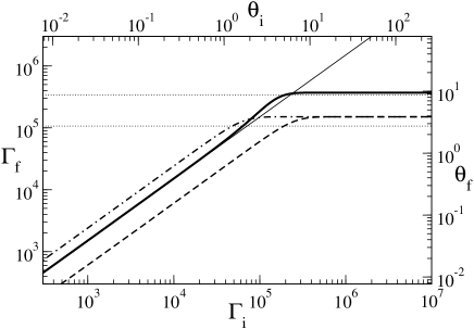
Figure 3: Final scaled temperature as a function of the initial scaled temperature for $r_{\rm s}=2\cdot 10^{9}$ and for $\omega_{\rm L}/\omega_{0}=1$ (thick solid line), $\omega_{\rm L}/\omega_{0}=2$ (dashed line) and $\omega_{\rm L}/\omega_{0}=1/2$ (dot-dashed line). For comparison, the result obtained with the classical expressions for initial- and final-state energies is shown by the thin solid line. The horizontal dotted lines show the estimate equation (11) for the limiting temperature.

$\Gamma_{\rm i}$ for $r_{\rm s}=2\cdot 10^{9}$. In contrast to the classical case, here the final temperature cannot be decreased to arbitrarily low values, rather it approaches a finite constant value as $T_{\rm i}\rightarrow 0$, since the initial charge distributions at the lattice sites have a finite extension at $T_{\rm i}=0$ due to zero-point oscillations. Using the low-temperature limit equation (8) as an estimate for the final energy and neglecting terms of order $\nu^{2}$ in the resulting energy balance, this limiting temperature is found to be

$$\frac{k_{\rm B}T_{\rm f}}{\hbar\omega_{0}}=\frac{1}{2}\frac{\omega_{\rm L}}{\omega_{0}}+\frac{1}{2}\frac{\omega_{0}}{\omega_{\rm L}}-\Omega,$$ (11)

where $\Omega=0.886-0.243/\sqrt{r_{\rm s}}$. Since $\Omega<0.886$ independent of $r_{\rm s}$, the limiting temperature is always positive and takes on a minimum value of

$$\left(\frac{k_{\rm B}T_{\rm f}}{\hbar\omega_{0}}\right)_{\rm{min}}=1-\Omega\stackrel{{\scriptstyle r_{\rm s}\gg 1}}{{\longrightarrow}}0.114$$ (12)

at an optimum ratio of $\omega_{\rm L}$ and $\omega_{0}$ of

$$\left(\frac{\omega_{\rm L}}{\omega_{0}}\right)_{\rm{min}}=1\;.$$ (13)

Note, however, that the limiting temperature obtained numerically with the full expression for $w_{\rm{f}}$ is slightly smaller since at finite temperature the system will not be in the groundstate, hence its potential energy is somewhat larger than that given by equation (8). We may rewrite equation (12) as $\lambda_{\rm T}/a=\sqrt{2\pi/[\sqrt{r_{\rm s}}(1-\Omega)]}\stackrel{{\scriptstyle r_{\rm s}\gg 1}}{{\longrightarrow}}7.424r_{\rm s}^{-1/4}$, where $\lambda_{\rm T}=h/\sqrt{2\pi Mk_{\rm B}T_{\rm f}}$ is the thermal deBroglie wavelength. This would suggest that it is possible to reach the degenerate regime of $\lambda_{\rm T}/a\approx 1$ if $r_{\rm s}$ can be decreased sufficiently, i.e. to a value $r_{\rm s}\approx 3\cdot 10^{3}$. Even for hydrogen this would correspond to an unrealistically large density of $4\cdot 10^{23}$cm^-3. Note, however, that the value of $r_{\rm s}$ enters the ratio $\lambda_{\rm T}/a$ with a power of $1/4$ only, so that values of $\lambda_{\rm T}/a=1/10$ can already be reached if $r_{\rm s}\approx 3\cdot 10^{7}$, corresponding to a density of $4\cdot 10^{11}$cm^-3, which has already been surpassed with cold Bose-condensed hydrogen atoms [25]. In this regime, the present considerations will not hold, since effects of particle statistics will be important which have not been included in the above expressions for the energies. However, equation (12) might serve as an estimate for the parameter values necessary to reach the degenerate regime.

In summary, we have discussed the possibility of correlation cooling and of the creation of a strongly coupled ultracold neutral plasma by photoionization of a highly ordered state of cold atoms, achievable with optical lattices. Classical considerations have shown that the initial temperature can be reduced by a factor of two if the atomic sample is noninteracting initially, offering the possibility to reach ion temperatures which have not been achieved so far. The quantum regime has been investigated using existing expressions for the equilibrium internal energy of the system. Here it was found that the final temperature approaches a constant value which arises from zero-point oscillations in the lattice potentials and depends on the density as well as the geometry of the optical lattice. An almost perfect lattice is necessary to observe the discussed cooling effects, since even a small amount of lattice defects largely increases the final temperature. However, it has been demonstrated that it is possible to create regular structures with a well-defined number of atoms localized in the potential wells of an optical lattice [26].

Financial support from the DFG through grant RO1157/4 is gratefully acknowledged.

References

References

- [1] Killian TC, Kulin S, Bergeson SD, Orozco LA, Orzel C and Rolston SL 1999 Phys. Rev. Lett.83 4776
- [2] Kulin S, Killian TC, Bergeson SD and Rolston SL 2000 Phys. Rev. Lett.85 318
- [3] Killian TC, Lim MJ, Kulin S, Dumke R, Bergeson SD and Rolston SL 2001 Phys. Rev. Lett.86 3759
- [4] Kuzmin SG and O’Neil TM 2002 Phys. Rev. Lett.88 065003
- [5] Robicheaux F and Hanson JD 2002 Phys. Rev. Lett.88 055002
- [6] Gericke DO and Murillo MS 2003 Contrib. Plasma Phys. 43 298
- [7] Murillo MS 2001 Phys. Rev. Lett.87 115003
- [8] Roberts JL, Fertig CD, Lim MJ and Rolston SL 2004 Preprint physics/0402041
- [9] Vanhaecke N, Comparat D, Tate DA and Pillet P 2004 Preprint quant-ph/0401045
- [10] Killian TC, Ashoka VS, Gupta P, Laha S, Nagel SB, Simien CE, Kulin S, Rolston SL and Bergeson SD 2003 J. Phys. A: Math. Gen.36 6077
- [11] Pohl T, Pattard T and Rost JM 2003 Preprint physics/0311131
- [12] Gericke DO, Murillo MS, Semkat D, Bonitz M and Kremp D 2003 J. Phys. A: Math. Gen.36 6087
- [13] Semkat D, Kremp D and Bonitz M 1999 Phys. Rev.E 59 1557
- [14] King IR 1966 Astron. J. 71 64
- [15] Simien CE, Chen YC, Gupta P, Laha S, Martinez YN, Mickelson PG, Nagel SB and Killian TC 2003 Preprint physics/0310017
- [16] Ichimaru S 1982 Rev. Mod. Phys.54 1017
- [17] Dubin DHE and O’Neil TM 1999 Rev. Mod. Phys.71 87
- [18] DeWitt H, Slattery W and Chabrier G 1996 Physica B 228 158
- [19] Chabrier G and Potekhin AY 1998 Phys. Rev.E 58 4941
- [20] Abe R 1959 Prog. Theor. Phys. 21 475
- [21] Schiffer JP 2002 Phys. Rev. Lett.88 205003
- [22] Hasse RW 2003 J. Phys. B: At. Mol. Opt. Phys.36 1011
- [23] Baiko DA, Potekhin AY and Yakovlev DG 2001 Phys. Rev.E 64 057402
- [24] Iyetomi H, Ogata S and Ichimaru S 1993 Phys. Rev.B 47 11703
- [25] Fried DG, Killian TC, Willmann L, Landhuis D, Moss SC, Kleppner D and Greytak TJ 1998 Phys. Rev. Lett.81, 3811
- [26] Greiner M, Mandel O, Esslinger T, Hänsch TW and Bloch I 2002 Nature 415 39