Capture into resonance in dynamics of a classical hydrogen atom in an oscillating electric field

Abstract

We consider a classical hydrogen atom in a linearly polarized electric field of slow changing frequency. When the system passes through a resonance between the driving frequency and the Keplerian frequency of the electron’s motion, a capture into the resonance can occur. We study this phenomenon in the case of 2:1 resonance and show that the capture results in growth of the eccentricity of the electron’s orbit. The capture probability for various initial values of the eccentricity is defined and calculated.

I Introduction

Dynamics of highly excited (Rydberg) atoms in microwave fields has been a subject of extensive research during the last thirty years. After experiments of Bayfield and Koch BK and theoretical work of Leopold and Percival LP , it was realised that certain essential properties of the dynamics of Rydberg hydrogen atoms can be described in the frames of classical approach.

One of the classical ideas in this area is to control the Keplerian motion of the electron using its resonant interaction with a wave of slowly changing frequency. Dynamical problems of this kind were studied in MF for a 1-D model and GF for a 3-D model. In particular, in the latter work an hydrogen atom in a linearly polarized electric field of slowly decreasing frequency was considered. It was shown that at a passage through 2:1 resonance (i.e., when the driving frequency is twice as large as the Keplerian frequency) the system with initially zero eccentricity of the electron’s orbit is captured into the resonance. In the captured state, the electron’s Keplerian frequency varies in such a way that the resonant condition is approximately satisfied. In this motion the orbit’s eccentricity grows, which may result in ionization of the atom.

In the present work we also consider a 3-D hydrogen atom in a linearly polarized electrostatic field of slowly changing frequency. We study behaviour of the system near 2:1 resonance using methods of the theory of resonant phenomena, developed in N75 - N99 (see also AKN ). These methods were previously used in studies of various physical problems including surfatron acceleration of charged particles in magnetic field and electromagnetic wave surfatron , slowly perturbed billiards bill1 , bill2 , and classical dynamics in a molecular hydrogen ion It2003 . In the present paper, we show that capture into the resonance necessarily occurs not only in the case of zero initial eccentricity but also if the initial eccentricity is not zero but small enough. Moreover, at larger values of the initial eccentricity the capture is also possible. Following the general approach, capture into the resonance in this case can be considered as a probabilistic phenomenon. We define and evaluate its probability. The obtained results can be used to broaden the applicability of the resonant control methods for Rydberg atoms.

The paper is organized as follows. In Section 2, we use standard techniques of classical celestial mechanics and the theory of resonant phenomena to reduce the equations of motion near the resonance to the standard form. We consider two different cases: one of small eccentricity and the other of eccentricity of order 1. In Section 3, we study the case of small eccentricity. We apply relevant results of N75 and find the region of so called ”automatic capture” into the resonance at small eccentricities and calculate probability of capture at larger values of initial eccentricity. Section 4 is devoted to the capture phenomenon at values of eccentricity of order 1. We calculate the capture probability in this case too. In the both cases, the capture significantly changes the eccentricity of the electron’s orbit and may lead to ionization. In Conclusions, we summarize the results.

II Equations of motion near the 2:1 resonance

We study dynamics of a classical electron in a hydrogen atom perturbed by a harmonically oscillating electric field of small amplitude $\mu$, linearly polarized along the $Z$-axis. This system is described with Hamiltonian

$${\cal H}={\cal H}_{0}+Z\mu\cos\Psi.$$ (1)

Here ${\cal H}_{0}$ is the unperturbed Hamiltonian of motion in the Coulomb field and $\Psi$ is the perturbation phase. Introduce the perturbation frequency $\omega=d\Psi/dt$. We assume that $\omega=\omega(\varepsilon t),\,0<\varepsilon\ll 1$, i.e. that this frequency slowly changes with time. For brevity, we put the electron mass and charge to 1, and use dimensionless variables.

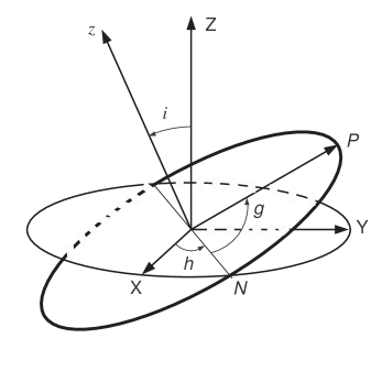
Figure 1: The Keplerian ellipse is shown with the bold line. The rest system of coordinates is $(XYZ)$, the $z$-axis is orthogonal to the plane of the orbit. The periapsis and the ascending node are denoted with P and N accordingly.

The unperturbed trajectory of the electron is an ellipse with eccentricity $e$, semimajor axis $a$, and inclination $i$. It is a well-known fact from celestial mechanics that the so-called Delaunay elements $L,G,H,l,g,h$ provide a set of canonical variables for the system under consideration (see, e.g. BrCl ). The Delaunay elements can be defined as

$$L=\sqrt{a},\;\;G=\sqrt{a(1-e^{2})},\;\;H=\sqrt{a(1-e^{2})}\cos i;$$ (2)

$l$ is the mean anomaly, $g$ is the argument of the periapsis, and $h$ is the longitude of the ascending node (see Figure 1).

In these variables, Hamiltonian (1) takes the form (see GF ):

$${\cal H} = {\cal H}_{0}+\mu{\cal H}_{1},\;\;{\cal H}_{0}=-\frac{1}{2L^{2}},$$

$${\cal H}_{1} = \sin i\sum^{\infty}_{k=1}\left[\frac{a_{k}+b_{k}}{4}\left(\sin(kl+g-\Psi)+\sin(kl+g+\Psi)\right)\right.+$$

$$\left.\frac{b_{k}-a_{k}}{4}\left(\sin(kl-g-\Psi)+\sin(kl-g+\Psi)\right)\right],$$

where

$$a_{k}=\frac{2a}{k}{\cal J}^{\prime}_{k}(ke),\;b_{k}=\frac{2a\sqrt{1-e^{2}}}{ke}{\cal J}_{k}(ke).$$ (4)

Here ${\cal J}_{k}(\cdot)$ is the Bessel function of integer order $k$, and ${\cal J}^{\prime}_{k}(\cdot)$ is its derivative.

In order to avoid possible singularities at $e=0$, we make a canonical transformation of variables $(L,G,H;l,g,h)\mapsto(P_{3},P_{2},P_{1};Q_{3},Q_{2},Q_{1})$ defined with generating function $P_{3}(l+g+h)+P_{2}(g+h)+P_{3}h$. The new canonical variables [called Poincaré elements of the first kind] are expressed in terms of the old ones as follows:

$$\begin{array}[]{cc}P_{3}=L,&Q_{3}=l+g+h,\\ P_{2}=G-L,&Q_{2}=g+h,\\ P_{1}=H-G,&Q_{1}=h.\end{array}$$ (5)

As the perturbation frequency slowly varies with time, the system passes through resonances with the unperturbed Keplerian frequency $\dot{l}$. Near a resonance, certain terms in expression (II) for ${\cal H}_{1}$ are changing very slowly. Consider a passage through the 2:1 resonance. In this case, after averaging over fast oscillating terms, we obtain the Hamiltonian describing the dynamics near the resonance:

$${\cal H}=-\frac{1}{2P_{3}^{2}}+\mu\,\alpha(P_{2},P_{3})\,\sin i\,\sin(2Q_{3}-Q_{2}-Q_{1}-\Psi),$$ (6)

where we introduced the notation $\alpha(P_{2},P_{3})=(a_{2}+b_{2})/4$.

The resonance is defined by $2\dot{Q}_{3}=\omega(\tau),\,\tau=\varepsilon t$. It follows from the unperturbed Hamiltonian (II) that $\dot{Q}_{3}=1/P_{3}^{3}$. Hence, denoting the value of $P_{3}$ at the resonance as $P_{r}$, we find:

$$P_{r}=\left(\frac{2}{\omega(\tau)}\right)^{1/3}.$$ (7)

Our next step is to introduce the resonant phase. We do this with the canonical transformation $(P_{i};Q_{i})\mapsto(J_{i};\gamma_{i}),\,i=1,2,3$ defined with the generating function

$$W=J_{3}(2Q_{3}-Q_{2}-Q_{1}-\Psi)+J_{2}Q_{2}+J_{1}Q_{1}.$$ (8)

For the new canonical variables we have

$$\begin{array}[]{cc}J_{3}=P_{3}/2,&\gamma_{3}=2Q_{3}-Q_{2}-Q_{1}-\Psi,\\ J_{2}=P_{2}+P_{3}/2,&\gamma_{2}=Q_{2},\\ J_{1}=P_{1}+P_{3}/2,&\gamma_{1}=Q_{1}.\end{array}$$ (9)

The Hamiltonian function takes the form:

$${\cal H}=-\frac{1}{8J_{3}^{2}}+\mu\,\alpha(J_{2},J_{3})\,\sin i\,\sin\gamma_{3}-\omega(\tau)J_{3}.$$ (10)

Near the resonant value $P_{3}=P_{r}$ we can expand this expression into series. With the accuracy of order $\mbox{O}(|P_{3}-P_{r}|^{3})$ we obtain the following Hamiltonian:

$${\cal F}=-\frac{3}{2}\frac{(P_{3}-P_{r})^{2}}{P_{r}^{4}}+\mu\,\alpha(J_{2},P_{3})\,\sin i\,\sin\gamma_{3},$$ (11)

where canonically conjugated variables are $P_{3}/2$ and $\gamma_{3}$. Introduce notations $P=P_{3},\varphi=\gamma_{3}+3\pi/2,J=J_{2}$. The Hamiltonian (11) does not contain $\gamma_{2}$, hence $J$ is an integral of the problem. Another integral is $J_{1}$, corresponding to the fact that Delaunay element $H$ is an integral of the original system (II). Coefficient $\sin i$ in (11) should be taken at $P=P_{r}$. We have

$$\left.\sin i\right|_{P=P_{r}}=\sqrt{1-\frac{H^{2}}{(J+P_{r}/2)^{2}}}.$$ (12)

From now on, we consider separately two different cases: the case of small initial eccentricity and the case when initial eccentricity is a value of order one. Let us start with the first case.

Assume the initial value of eccentricity is small, though not necessary zero. From (4), we have

$$\alpha(J,P)\approx\frac{ae}{4}=\frac{1}{4}P\sqrt{\left(\frac{P}{2}-J\right)\left(J+\frac{3}{2}P\right)}.$$ (13)

Small eccentricity implies that $P/2-J\ll 1$. As the system evolves near the resonance, small variations of $P$ are essential when calculating the term $(P/2-J)$ in (13) and less important in the other terms. Hence, in these latter terms, we can put $P=P_{r}$. We write

$$J+\frac{3}{2}P=\left(\frac{P}{2}-J+2J+P\right)\approx 2\left(J+\frac{P}{2}\right)\approx 2P,$$

where we have used that $P/2\approx J$. Thus, we obtain

$$\alpha(J,P)\approx\frac{\sqrt{2}}{4}P_{r}^{3/2}\sqrt{\frac{P}{2}-J}$$ (14)

and the following expression for the Hamiltonian:

$${\cal F}\approx{\cal F}_{1}=-\frac{3}{2}\frac{(P-P_{r})^{2}}{P_{r}^{4}}+\mu\sqrt{1-\frac{H^{2}}{(J+P_{r}/2)^{2}}}\,\frac{\sqrt{2}}{4}P_{r}^{3/2}\sqrt{\frac{P}{2}-J}\cos\varphi.$$ (15)

Introduce so-called Poincaré elements of the second kind:

$$x=\sqrt{P-2J}\cos\varphi,\;\;y=\sqrt{P-2J}\sin\varphi.$$ (16)

The transformation $(P/2,\varphi)\mapsto(x,y)$ is canonical with generating function $W_{1}=\frac{y^{2}}{2}\cot\varphi-J\varphi$. Change the sign of ${\cal F}_{1}$ and, to preserve the canonical form, the sign of $x$. Thus, we obtain the Hamiltonian in the form:

$${\cal F}_{1}=\frac{3}{2}\frac{(x^{2}+y^{2})^{2}}{P_{r}^{4}}-3\frac{x^{2}+y^{2}}{P_{r}^{4}}(P_{r}-2J)+\mu A(H,J,P_{r})x,$$ (17)

where

$$A(H,J,P_{r})=\frac{P_{r}^{3/2}}{4}\sqrt{1-\frac{H^{2}}{(J+P_{r}/2)^{2}}}.$$

Note, that if the eccentricity is small, then $P_{r}-2J\ll 1$, and hence the slow variation of $P_{r}$ is essential only in the second term in (17). In the other terms, $P_{r}$ can be assumed to be constant, say, $P_{r}=P_{r0}$, where $P_{r0}$ is the value of $P_{r}$ at $\tau=0$. Now, we renormalise the Hamiltonian ${\cal F}_{1}\to\frac{2}{3}P_{r0}^{4}{\cal F}_{1}$ to transform it to the following standard form studied in N75 :

$${\cal F}_{1}=(x^{2}+y^{2})^{2}-\lambda(x^{2}+y^{2})+\tilde{\mu}x$$ (18)

with $\lambda=2(P_{r}-2J)$ and $\tilde{\mu}=\mu A(H,J,P_{r0})$. We describe the dynamics defined by Hamiltonian (18) in Section 3.

Return now to equation (11) and consider the case when the eccentricity is not small: $e\sim 1$. In this case we can put $P=P_{r}$ when calculating $\alpha$. Thus we obtain

$${\cal F}\approx{\cal F}_{2}=-\frac{3}{2}\frac{(P-P_{r})^{2}}{P_{r}^{4}}+\mu B(H,J,P_{r})\cos\varphi,$$ (19)

where

$$B(H,J,P_{r})=\sin i\,\alpha(J,P_{r})=\sqrt{1-\frac{H^{2}}{(J+P_{r}/2)^{2}}}\,\frac{1}{4}\left[a{\cal J}^{\prime}_{2}(2e)+\frac{a\sqrt{1-e^{2}}}{e}{\cal J}_{2}(2e)\right],$$ (20)

and values of $a$ and $e$ are calculated at $P=P_{r}$:

$$a=P_{r}^{2},\;\;\;e=\sqrt{1-\frac{(J+P_{r}/2)^{2}}{P_{r}^{2}}}.$$ (21)

The system with Hamiltonian function (19) is a pendulum with slowly changing parameters. We study the dynamics in this system in Section 4.

III Capture into the resonance at small values of eccentricity

Dynamics in the system with Hamiltonian function (18) was studied in details in N75 . In this section we put forward the results of N75 relevant to our study.

In (18) $\tilde{\mu}>0$ is a constant parameter, and $\lambda$ is a slow function of time, $\dot{\lambda}\sim\varepsilon$. Assume that $\dot{\lambda}>0$.

On the phase plane $(x,y)$, the values $\sqrt{P-2J}$ and $\varphi$ (see (16)) are polar coordinates. Note that eccentricity in the original problem is proportional to $\sqrt{P-2J}$.

Parameter $\lambda$ is changing slowly, and as the first step we consider the problem at fixed values of $\lambda$. Phase portraits at different values of $\lambda$ are presented in Figures 2, 3. At $\lambda<\lambda_{*}=\frac{3}{2}\tilde{\mu}^{2/3}$ (Figure 2a) there is one elliptic stable point A on the portrait. At $\lambda>\lambda_{*}$ (Figure 3) there are two elliptic stable points A and B, and one saddle point C. Separatrices $l_{1},l_{2}$ divide the phase plane into three regions $G_{1},G_{12},G_{2}$. In Figure 2b, the portrait at $\lambda=\lambda_{*}$ is shown.

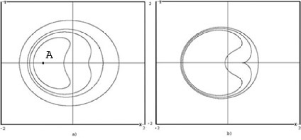
Figure 2: Phase portraits of the system at fixed values of $\lambda$; $\tilde{\mu}=0.01$. a) $\lambda=0.05<\lambda_{*}$, b) $\lambda=0.069624\approx\lambda_{*}$.

The coordinates of point C are $x=x_{c},y=0$, where $x_{c}=x_{c}(\lambda)$ is the largest root of equation

$$\frac{\partial{\cal F}_{1}(x,0,\lambda)}{\partial x}=4x^{3}-2\lambda x+\tilde{\mu}=0.$$ (22)

At $\lambda\geq\lambda_{*}$, introduce $F_{c}=F_{c}(\lambda)={\cal F}_{1}(x_{c},0,\lambda)$ and $\tilde{\cal F}(x,y,\lambda)={\cal F}(x,y,\lambda)-F_{c}(\lambda)$. In $G_{12}$ we have $\tilde{\cal F}<0$, in $G_{1}$ and $G_{2}$ $\tilde{\cal F}>0$, on the separatrices $\tilde{\cal F}=0$.

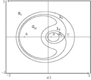
Figure 3: Phase portrait of the system at $\lambda=0.1>\lambda_{*}$; $\tilde{\mu}=0.01$.

As parameter $\lambda$ slowly grows with time, $\dot{\lambda}\sim\varepsilon$, curves $l_{1},l_{2}$ defined with $\tilde{\cal F}=0$ slowly move on the phase plane. On time intervals of order $\varepsilon^{-1}$ their position on the phase plane essentially changes, together with the areas of $G_{12},G_{2}$. On the other hand, area surrounded by a closed phase trajectory at a frozen value of $\lambda$ is an approximate integral [adiabatic invariant] of the system with slowly varying parameter $\lambda$. Therefore, a phase point can cross $l_{1},l_{2}$ leaving one of the regions $G_{i}$ and entering another region.

Denote with $(x(t),y(t))$ a phase point moving according to (18). Without loss of generality assume that $\lambda=\lambda_{*}$ at $t=0$. The initial point $(x(0),y(0))$ can be either inside $l_{1}$ [$\tilde{\cal F}_{0}=\tilde{\cal F}(x(0),y(0),\lambda_{*})<0$] or out of $l_{1}$ [$\tilde{\cal F}_{0}>0$]. The following assertion is valid. All points lying inside $l_{1}$ at $\lambda=\lambda_{*}$ except, maybe, of those belonging to a narrow strip $-k_{1}\varepsilon^{6/5}\leq\tilde{\cal F}_{0}<0$, where $k_{1}$ is a positive constant, stay in $G_{12}$ at least during time intervals of order $\varepsilon^{-1}$.

This result is due to the fact that the area of $G_{12}$ monotonously grows with time, and conservation of the adiabatic invariant makes a phase point go deeper and deeper into this region. A point captured in $G_{12}$ rotates around point A$=(x_{A},0)$, where $x_{A}$ is the smallest root of equation (22). As time grows, $|x_{A}|$ also grows and point A on the portrait slowly moves along $x$-axis in the negative direction. Therefore, the motion is a composition of two components: fast rotation along a banana-shaped curve surrounding A and slow drift along $x$-axis. The area surrounded by each banana-shaped turn is approximately the same and equals the area ${\cal S}(\lambda_{*})$ surrounded by the trajectory passing through $(x(0),y(0))$ at $\lambda=\lambda_{*}$. Hence, the average distance between the phase point and the origin slowly grows, corresponding to the eccentricity growth in the original problem.

In GF , it was shown that a point having zero initial eccentricity necessarily undergoes the eccentricity growth. The formulated result implies that this is also valid for all the points initially [i.e., at $\lambda=\lambda_{*}$] inside $l_{1}$, except, maybe for a narrow strip close to $l_{1}$. A typical linear size of this domain is of order $\tilde{\mu}^{1/3}$. In Sincl this phenomenon was described and called ”automatic entry into libration”.

Consider now the case when the point $(x(0),y(0))$ is outside $l_{1}$: $\tilde{\cal F}_{0}>0$. With time the area inside $l_{1}$ grows, and at a certain moment the phase trajectory crosses $l_{1}$. In the adiabatic approximation the area surrounded by the phase trajectory is constant: ${\cal S}(\lambda)={\cal S}(\lambda_{*})$. Hence, in this approximation the time moment of crossing $l_{1}$ can be found from equation ${\cal S}_{1}(\Lambda)={\cal S}(\lambda_{*})$. Here ${\cal S}_{1}(\lambda)$ is the area inside $l_{1}$ as a function of $\lambda$ and $\Lambda$ is a value of the parameter at this moment. After crossing, there are two possibilities: (i) the phase point can continue its motion in $G_{12}$ during a time interval of order at least $\varepsilon^{-1}$ [this corresponds to capture into the resonance and growth of the eccentricity]; (ii) without making a full turn inside $G_{12}$ the phase point can cross $l_{2}$ and continue its motion in $G_{2}$ [this corresponds to passage through the resonance without capture]. The area of $G_{2}$ also monotonously grows with time, hence such a point can not cross $l_{2}$ once more and return to $G_{12}$

It is shown in N75 that the scenario of motion after crossing $l_{1}$ strongly depends on initial conditions $(x(0),y(0))$: a small, of order $\varepsilon$, variation of initial conditions can result in qualitatively different evolution. If the initial conditions are defined with a final accuracy $\delta$, $\varepsilon\ll\delta\ll 1$, it is impossible to predict a priori the scenario of evolution. Therefore, it is reasonable to consider capture into $G_{12}$ or $G_{2}$ as random events and introduce their probabilities.

Following Arn63 , consider a circle of small radius $\delta$ with the centre at the initial point M₀. Then the probability of capture into $G_{12}$ is defined as

$${\cal P}=\lim_{\delta\to 0}\;\lim_{\varepsilon\to 0}\;\frac{S_{12}}{S_{M_{0}}^{\delta}},$$ (23)

where $S_{M_{0}}^{\delta}$ is the measure of the circle of radius $\delta$ and $S_{12}$ is the measure of the points inside this circle that are captured finally into $G_{12}$.

Let $\lambda=\Lambda$ be the parameter value at the moment of crossing $l_{1}$ in the adiabatic approximation. The following formula for probability $P$ is valid:

$${\cal P}=\frac{I_{1}-I_{2}}{I_{1}},\;\;\mbox{where}\;I_{1}(\lambda)=-\oint_{l_{1}}\frac{\partial\tilde{\cal F}}{\partial\lambda}\mbox{d}t,\;\;I_{2}(\lambda)=-\oint_{l_{2}}\frac{\partial\tilde{\cal F}}{\partial\lambda}\mbox{d}t,$$ (24)

and the integrals $I_{1},I_{2}$ are calculated at $\lambda=\Lambda$. Calculating the integrals, one finds N75

$$I_{1}(\Lambda)=\frac{1}{2}(2\pi-\Theta),\;\;I_{2}=\frac{\Theta}{2},\;\;\Theta=\arccos\left(\frac{\Lambda}{2x_{c}^{2}}-2\right).$$ (25)

Here $\Theta$ is the angle between the tangencies to $l_{1}$ at C, $0\leq\Theta<\pi$.

Geometrically, formula (24) can be interpreted as follows. In a Hamiltonian system, phase volume is invariant. As parameter $\lambda$ changes by $\Delta\lambda$, a phase volume $\Delta V_{12}$ enters the region $G_{12}$. At the same time, a volume $\Delta V_{2}$ leaves this region and enters $G_{2}$. The relative measure of points captured in $G_{12}$ is $(\Delta V_{12}-\Delta V_{2})/\Delta V_{2}$. The integral $I_{1}$ in (24) is the flow of the phase volume across $l_{1}$, and $I_{2}$ is the flow across $l_{2}$. Therefore, ${\cal P}$ gives the relative measure of points captured into $G_{12}$.

Note that, rigorously speaking, there also exists a set of initial conditions that should be excluded from consideration. Phase trajectories with initial conditions in this set pass very close to saddle point C, and the asymptotic results of N75 cannot be applied to them. However, this exclusive set is small: it is shown in N75 that its relative measure is a value of order $\sqrt{\varepsilon}$.

In Figure 4a, capture into the resonance is shown. First, the phase point rotates around the origin in region $G_{1}$, then it crosses $l_{1}$, enters region $G_{12}$ and continues its motion in this region. In the course of this motion, the average distance from the origin grows, corresponding to the growth of the eccentricity. In Figure 4b, all the parameter values are the same as in Figure 4a, but initial conditions are slightly different. In this case, after crossing $l_{1}$, the phase point crosses $l_{2}$ and gets into region $G_{2}$. This is a passage through the resonance without capture.

Figure 4: Passage through the resonance on $(x,y)$-plane and corresponding variation of eccentricity (bottom plots, Ecc denotes $(x^{2}+y^{2})^{1/2}$); $\tilde{\mu}=0.01,\varepsilon=0.01$. a) Passage with capture into the resonance; b) passage without capture; initial conditions in the cases a) and b) are different.

Summarizing the results of this section, we can say the following. (i) Capture into the resonance in the considered case results in growth of the eccentricity of the electron’s orbit. (ii) On the phase plane around the origin [$e=0$], there exists a region of size of order $\tilde{\mu}^{1/3}$ such that all phase trajectories with initial conditions [i.e. at $\lambda=\lambda_{*}$] in this region undergo a capture into the resonance with necessity [”automatic capture”]. (iii) If initial eccentricity is larger, and the initial point on the phase plane is out of the region mentioned above, there is a finite probability that the phase trajectory will be captured into the resonance. This probability is given by (24).

IV Capture into the resonance at eccentricity of order 1.

If initial eccentricity is a value of order one, dynamics in a $\sqrt{\mu}$-neighbourhood of the resonance is described by Hamiltonian (19). In this Hamiltonian, $P_{r}=P_{r}(\tau)$ is a monotonously increasing function of the slow time $\tau=\varepsilon t$. At a frozen value of $P_{r}$, this is a Hamiltonian of a pendulum, with elliptic points at $P=P_{r},\,\varphi=0\,\mbox{mod}\,2\pi$ and hyperbolic points at $P=P_{r},\,\varphi=\pi\,\mbox{mod}\,2\pi$. Denote the value of the Hamiltonian at hyperbolic points with $F_{s}$. The separatrices connecting the hyperbolic points with $\varphi=-\pi$ and $\varphi=\pi$ are defined by equation ${\cal F}_{2}=F_{s}$ or:

$$P-P_{r}=\pm\sqrt{2/3}\,P_{r}^{2}\,\sqrt{\mu B(H,J,P_{r})}\,\sqrt{1+\cos\varphi}.$$ (26)

The separatrices divide the phase cylinder $P\in\mathbb{R},\,\varphi\in\mathbb{S}^{1}$ into domains of direct rotation, oscillation, and reverse rotation. The area $S$ of the oscillatory domain is proportional to $P_{r}^{2}\sqrt{\mu B}$; it can be shown that it is a monotonically growing function of $P_{r}$.

Now take into consideration the slow growth of $P_{r}$ with time. This growth produces slow motion of the phase portrait upwards on the phase cylinder. At the same time the area between the separatrices slowly grows. As a result, phase point initially above the upper separatrix, i.e. in the domain of direct rotation, can cross the separatrix and be either captured into the oscillatory domain (this is a capture into the resonance), or pass through to the domain of reverse rotation. The final mode of motion strongly depends on initial conditions: a small, of order $\varepsilon$, variation in them can result in qualitatively different final mode of motion. Thus, like in the situation described in Section 3, capture into the oscillatory domain in this problem can be considered as a probabilistic phenomenon. The probability of capture can be found as follows. As parameter $P_{r}$ changes by a small value $\Delta P_{r}$, phase volume $\Delta V=(\frac{\mbox{d}S}{\mbox{d}P_{r}}+L)\Delta P_{r}$, where $L$ is the length of the separatrix, crosses the upper separatrix. In the latter expression, the first term is due to the growth of the area of the oscillatory domain, and the second term is due to the slow motion of the upper separatrix on the phase portrait. At the same time, phase volume $\Delta V_{+}=\frac{\mbox{d}S}{\mbox{d}P_{r}}\Delta P_{r}$ enters the oscillatory domain and stays inside of it. Hence, the probability of capture can be evaluated as

$${\cal P}=\frac{\Delta V_{+}}{\Delta V}.$$ (27)

Straightforward calculations give:

$${\cal P}=\frac{\sqrt{\mu}P_{r}^{2}K}{\sqrt{\mu}P_{r}^{2}K+\sqrt{1+\mu P_{r}^{6}\tilde{K}}},$$ (28)

where $K$ and $\tilde{K}$ are bounded functions of $P_{r}$ (we do not write the full expressions here explicitly for brevity). It can be shown (see N93 ) that asymptotically as $\varepsilon\to 0$ (27) gives the correct value of ${\cal P}$ defined as in (23) with $S_{12}$ denoting the measure of captured points inside a small circle of initial conditions. At $\mu\ll P_{r}^{-6}$, we find from (28) that ${\cal P}\sim\sqrt{\mu}$.

For a captured phase point value of $P$ remains at a distance of order $\sqrt{\mu}$ from $P_{r}$ on time intervals of order $\varepsilon^{-1}$. Therefore, as it follows from expressions (21), as $P_{r}$ grows, the eccentricity along the captured phase trajectory tends to $\sqrt{3}/2$, and the semimajor axis of the electron’s orbit tends to infinity. At $J>0$, the eccentricity is always smaller than $\sqrt{3}/2$, and at $J<0$ it is always larger than $\sqrt{3}/2$. Note, however, that in the original system, as it follows from (7), the rate of variation of $P_{r}$ is large at large values of $P_{r}$. Therefore, strictly speaking, the asymptotic methods used in this section are not applicable in the limit $P_{r}\to\infty$.

In Figure 5a, capture into the resonance is shown. In the beginning, the phase trajectory encircles the phase cylinder at approximately constant initial value of $P$. Then the phase point crosses the upper separatrix of the pendulum (19), and enters the oscillatory domain. Since this moment, the phase trajectory does not encircle the phase cylinder and the average value of $P$ grows. The eccentricity also grows. Figure 5b shows a passage through the resonance without capture. The phase point does not stay in the oscillatory domain, but crosses the bottom separatrix and enters the domain of reverse rotation and continues its motion at approximately constant new value of $P$. In this case, the eccentricity undergoes only a small variation.

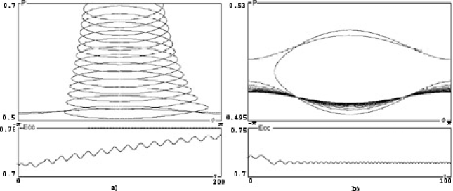
Figure 5: Passage through the resonance on the $(P,\varphi)$ phase cylinder and corresponding variation of the eccentricity (bottom plots, Ecc denotes $\sqrt{1-\frac{(J+P/2)^{2}}{P^{2}}}$); $\mu=0.1,\varepsilon=0.001,J=0.1,H=0.2$. Initial conditions are different in the cases a) and b).

V Conclusions

We have shown that if the frequency of the driving field slowly decreases, there always exists a certain probability of capture into the resonance. A capture results in strong variation of the electron orbit’s eccentricity, and may lead to ionisation of the atom. The resonant capture mechanism is a good tool for control of behaviour of Rydberg atoms. Note, that even if the capture probability is small (as in the case considered in Section 4), the phenomenon is still important. Consider, for example, an ensemble of Rydberg atoms with various initial eccentricities in the case when the driving frequency changes slowly periodically. Then, after large enough number of these periods, a relative number of order one of the atoms undergo the capture. If the capture probability is a value of order $\sqrt{\mu}$, it will happen after $\mbox{O}(\mu^{-1/2})$ periods, which needs time of order $\varepsilon^{-1}\mu^{-1/2}$.

References

- (1) J.E.Bayfield and P.M.Koch, Phys. Rev. Lett. 33, 258 (1974)
- (2) J.G.Leopold and I.C.Percival, Phys Rev. Lett. 41, 944 (1978)
- (3) B.Meerson and L.Friedland, Phys. Rev. A 41, 5233 (1990)
- (4) E.Grosfeld and L.Friedland, Phys. Rev. E 65, 046230 (2002)
- (5) A.I.Neishtadt, Prikl. Mat. Mech 39, 1331 (1975)
- (6) A.I.Neishtadt, Selecta Mathematica formerly Sovetica 12 No. 3 (1993) 195-210
- (7) A.I.Neishtadt, Celestial Mech. and Dynamical Astronomy 65 (1997) 1-20.
- (8) A.I.Neishtadt, In: ”Hamiltonian systems with three or more degrees of freedom”, Ed. C.Simo, NATO ASI Series, Series C, vol. 533, Kluwer Academic Publishers, Dordrecht/Boston/London, 1999, 193-213.
- (9) V.I.Arnold, V.V.Kozlov and A.I.Neishtadt, (1988) Mathematical aspects of classical and celestial mechanics (Encyclopaedia of mathematical sciences 3) (Berlin: Springer).
- (10) A.P.Itin, A.I.Neishtadt, A.A.Vasiliev, Physica D 141 (2000) 281-296.
- (11) A.P.Itin, A.I.Neishtadt, A.A.Vasiliev, Physics Letters A 291 (2001) 133-138.
- (12) A.P.Itin, A.I.Neishtadt, Regular and Chaotic Dynamics, No.2 (2003).
- (13) A.P.Itin, Phys. Rev. E 67, 026601 (2003)
- (14) D.Brouwer and G.Clemens, (1961) Methods of celestial mechanics (Academic Press, New York and London).
- (15) A.T.Sinclair, Month. Notic. Roy. Astron. Soc. 160, No.2 (1972) 169-187.
- (16) V.I.Arnol’d, Russ. Math. Surveys 18 (1963) 85-192.