Electromagnetic wave scattering from a random layer with rough interfaces II: Diffusive intensity

Abstract

A general approach for the calculation of the incoherent intensity scattered by a random medium with rough boundaries has been developed using a Green function formalism. The random medium consists of spherical particles whose physical repartition is described by a pair-distribution function. The boundary contribution is included in the Green functions with the help of scattering operators which can represent any existing theory of scattering by rough surfaces. By using a standard procedure, we derive the integral Bethe-Salpeter equation under the ladder approximation and, by differentiation, the vectorial radiative transfer equation. Furthermore, with the help of our formalism, the boundary conditions necessary to solve the radiative transfer equation are expressed in terms of the scattering operators of the rough surfaces. Finally, using the reciprocity properties of the Green functions, we are able to include the enhanced backscattering contributions to take into account every state of polarization of the incident and the scattered waves.

1 Introduction

In the preceding paper [1] (referred as I), we have developed a general formalism based on Green functions to calculate the electromagnetic field scattered by a random medium with rough boundaries. In using these Green functions, we have determined the average electric field, also named the coherent field. In this paper, we use the formalism developed in I to calculate the diffusive intensity also named incoherent intensity.

The study of electromagnetic wave propagation through random media has been an intensive field of research for many decades [2, 3, 4, 5, 6, 7, 8, 9, 10, 11, 12, 13, 14, 15, 16]. Many aspects of the transport of waves in such media are well described by the phenomenological radiative transfer theory [2, 5, 6, 7, 9, 10, 14, 16]. In this approach, the main quantity, used to describe the propagation, is the specific intensity $\mathcal{I}(\boldsymbol{R},\hat{\boldsymbol{k}})$ (if we take into account the polarization of the wave, the specific intensity can be defined as a Stokes vector or a tensor) which gives the power flux per unit area and solid angle at the point $\boldsymbol{R}$ which goes in the direction $\hat{\boldsymbol{k}}$. In writing a balance equation on the energy, it is shown that the specific intensity satisfies a Boltzmann type equation called radiative transfer equation. If the particles are inside a slab with a permittivity different from the surrounding medium, boundary conditions must be added to the radiative transfer equation in order to calculate the specific intensity. For rough surfaces, these boundary conditions are expressed with scattering operators, where several approximate analytical expressions exist depending on the roughness of the surface. Numerical calculations of the radiative transfer equation taking into account rough boundaries can be found in references [7, 12, 17, 18]

However, all previous studies on the radiative transfer theory are based on heuristic principles since in these works, the specific intensity is a fundamental quantity which is not defined from the electromagnetic field $\boldsymbol{E}$ and $\boldsymbol{B}$. The link between the electromagnetism and the classical radiometry theory is due to Walther [19] who has first recognized that the specific intensity can be deduced from the Wigner function $\boldsymbol{\mathcal{I}}(\boldsymbol{R},\boldsymbol{k})=Const\times\int\rmd^{3}\boldsymbol{r}\,\exp(-\rmi\boldsymbol{k}\cdot\boldsymbol{r})\,\boldsymbol{E}(\boldsymbol{R}+\boldsymbol{r}/2)\otimes\boldsymbol{E}^{*}(\boldsymbol{R}-\boldsymbol{r}/2)$, where the tensorial product $\otimes$ permit to take into account the different polarizations of the waves. If we suppose that the electric field depends slightly on the coordinates $\boldsymbol{R}$ compared to $\boldsymbol{r}$ (quasi-uniform fields hypothesis [13]), it is shown that the Wigner function is written as $\boldsymbol{\mathcal{I}}(\boldsymbol{R},\boldsymbol{k})=Const\times\delta(||\boldsymbol{k}||-K_{0})\,\boldsymbol{\mathcal{I}}(\boldsymbol{R},\hat{\boldsymbol{k}})$, where $\hat{\boldsymbol{k}}=\boldsymbol{k}/||\boldsymbol{k}||$ and $K_{0}$ the wavenumber. In this case, the function $\boldsymbol{\mathcal{I}}(\boldsymbol{R},\hat{\boldsymbol{k}})$ can be identified with the specific intensity. Nevertheless, there are some differences between this definition of the specific intensity with the radiometric one. In fact, this electromagnetic definition of the specific intensity is not always a positive function, which is in contradiction with the radiometric interpretation in terms of power. This problem has been the subject of much study [13, 20, 21] where it has been demonstrated that in the geometrical limit, the electromagnetic definition of the specific intensity is always positive. In other cases, the negative value of the specific intensity are due to interference effects.

As soon as we have determined the relationship between the electromagnetic field and the specific intensity, we can derive the radiative transfer equation from the Maxwell equations. The procedure is to write the Maxwell equations in an integral form with the help of Green functions and to apply the Wigner transform to the equation derived. Then, in differentiating this equation we obtain the radiative transfer equation [22, 23, 24, 25, 26, 27, 28, 29, 30, 31, 32, 33, 34, 35]. Furthermore, in starting from the wave equations, we are able to take into account new contributions to the scattered intensity such as the enhanced backscattering and the correlations between the scatterers that can not be introduced in the phenomenological radiometric approach. The objective of this paper is to derive the radiative transfer equation from the wave equation by taking into account rough boundaries. Several works have investigated this topics, but they describe the scattering by the rough surfaces either by using the small-perturbation method [36, 37, 38] or in an unconventional fashion [39, 40]. In our approach, we use scattering operators which are a versatile and unified way to describe how the wave interacts with the boundaries  [41]. To use these operators, we have introduced two kinds of Green functions (I). The first one $\overline{\boldsymbol{G}}_{SV}(\boldsymbol{r},\boldsymbol{r}_{0})$ describes the field scattered by the volume (V), which contains the scatterers, and by the rough surfaces (S). The second type of Green function is $\overline{\boldsymbol{G}}_{S}(\boldsymbol{r},\boldsymbol{r}_{0})$, which describes the field scattered by a slab with rough boundaries where the scatterers have been replaced by an homogeneous medium of permittivity $\epsilon_{e}$ named effective permittivity. As demonstrated in I, the Green functions $\overline{\boldsymbol{G}}_{S}(\boldsymbol{r},\boldsymbol{r}_{0})$ are easily expressed as a function of the rough surface scattering operators. In using these kind of Green functions, we were able to separate the contribution coming from the surface and the volume. The main advantage of our approach is that the equations obtained are similar to the equations generally used to describe the wave scattered by an infinite random medium [9, 24, 25, 27, 34]. To take into account the boundaries, we replace the Green function of an infinite homogeneous random medium with $\overline{\boldsymbol{G}}_{S}(\boldsymbol{r},\boldsymbol{r}_{0})$. Yet, there is a slightly difference from the classical procedure. Usually, we use the normalized vector $\hat{\boldsymbol{k}}$ ($||\hat{\boldsymbol{k}}||=1$) to describe the propagation direction of the wave since the generalized Dirac function in the specific intensity $\overline{\boldsymbol{\mathcal{I}}}(\boldsymbol{r},\boldsymbol{k})$ imposes that $\boldsymbol{k}=K_{0}\,\hat{\boldsymbol{k}}$. In this study, we will use the two-dimensional vector $\boldsymbol{p}=k_{x}\hat{\boldsymbol{e}}_{x}+k_{y}\hat{\boldsymbol{e}}_{z}$ to describe the propagation direction, and we will recover the vector $\hat{\boldsymbol{k}}$ by following decomposition: $K_{0}\hat{\boldsymbol{k}}=\boldsymbol{p}+a\alpha_{0}(\boldsymbol{p})\hat{\boldsymbol{e}}_{z}$, where $\alpha_{0}(\boldsymbol{p})=(K_{0}^{2}-\boldsymbol{p}^{2})^{1/2}$, and $a$ is the sign of the vertical component of $\hat{\boldsymbol{k}}$ ($a=\mathrm{sgn}(\hat{\boldsymbol{k}}\cdot\hat{\boldsymbol{e}}_{z})$). This choice, which is unusual for the radiative transfer theory, is in fact the standard in scattering by rough boundaries where the vertical axis $z$ has to be differentiated from the axis $\boldsymbol{x}=x\hat{\boldsymbol{e}}_{x}+y\hat{\boldsymbol{e}}_{y}$ for a surface profile defined by $z=h(\boldsymbol{x})$ [41]. Furthermore, the distinction between upward waves for $a=+$ and downward waves for $a=-$ is useful to write the boundary conditions. At the end of this paper, we will explain how to rewrite the equations obtained in the usual form with $\hat{\boldsymbol{k}}$ vectors.

2 Cross-section

The geometry of the problem and the notation are described in paper I. In order to characterize the scattered intensity by an object, we usually introduce the bistatic cross-section, which is the power scattered per solid angle normalized by the incident power flux. In this paper, we will use a generalization of this concept called Muller bistatic cross-section, which permits an accounting for every state of polarization of the incident and scattered waves. First, as an intermediate of calculation, we have to introduce the scattering operators describing the field scattered by the rough surfaces and the random media . For an incident plane wave,

$$\boldsymbol{E}^{0i}(\boldsymbol{r})=\boldsymbol{E}^{0i}(\boldsymbol{p}_{0})\,\rme^{\rmi\,\boldsymbol{p}_{0}\cdot\boldsymbol{x}-\rmi\,\alpha_{0}(\boldsymbol{p}_{0})z}\,,$$ (1)

the field scattered by the random medium and the rough boundaries is:

$$\boldsymbol{E}^{0s}_{SV}(\boldsymbol{r})=\int\frac{\rmd^{2}\boldsymbol{p}}{(2\pi)^{2}}\,\rme^{\rmi\,\boldsymbol{p}\cdot\boldsymbol{x}+\rmi\,\alpha_{0}(\boldsymbol{p})z}\,\overline{\boldsymbol{R}}_{SV}(\boldsymbol{p}|\boldsymbol{p}_{0})\cdot\boldsymbol{E}^{0i}(\boldsymbol{p}_{0})\,,$$ (2)

where $\alpha_{0}(\boldsymbol{p})=\sqrt{K_{0}^{2}-\boldsymbol{p}^{2}}$, and using the notation defined in I, we decompose the vector $\boldsymbol{E}^{0i}(\boldsymbol{p}_{0})$ and the dyad $\overline{\boldsymbol{R}}_{SV}(\boldsymbol{p}|\boldsymbol{p}_{0})$ on the following basis:

$$\boldsymbol{E}^{0i}(\boldsymbol{p}_{0}) =\sum_{\beta=H,V}E^{0i}(\boldsymbol{p}_{0})_{\beta}\,\hat{\boldsymbol{e}}^{0-}_{\beta}(\boldsymbol{p}_{0})$$ (3)

$$\overline{\boldsymbol{R}}_{SV}(\boldsymbol{p}|\boldsymbol{p}_{0}) =\sum_{\beta,\beta_{0}=H,V}R_{SV}(\boldsymbol{p}|\boldsymbol{p}_{0})_{\beta,\beta_{0}}\,\hat{\boldsymbol{e}}^{0+}_{\beta}(\boldsymbol{p})\hat{\boldsymbol{e}}^{0-}_{\beta_{0}}(\boldsymbol{p}_{0})\,,$$ (4)

where the polarization vector $\hat{\boldsymbol{e}}^{0\pm}_{\beta_{0}}(\boldsymbol{p})$ for the polarization TM ($\beta=V$) and the polarization TE ($\beta=H$) are defined by

$$\hat{\boldsymbol{e}}_{V}^{0\pm}(\boldsymbol{p})=\pm\frac{\alpha_{0}(\boldsymbol{p})}{K_{0}}\hat{\boldsymbol{p}}-\frac{||\boldsymbol{p}||}{K_{0}}\hat{\boldsymbol{e}}_{z}\,,\qquad\hat{\boldsymbol{e}}_{H}(\boldsymbol{p})=\hat{\boldsymbol{e}}_{z}\times\hat{\boldsymbol{p}}\,.$$ (5)

Far from the scattering medium ($K_{0}||\boldsymbol{r}||\gg 1$), we can obtain an asymptotic expression of the integral in equation (2) by using the stationary phase approximation [42]:

$$\boldsymbol{E}^{0s}_{SV}(\boldsymbol{r})=\frac{\rme^{\rmi K_{0}||\boldsymbol{r}||}}{||\boldsymbol{r}||}\,\overline{\boldsymbol{f}}(\boldsymbol{p}|\boldsymbol{p}_{0})\cdot\boldsymbol{E}^{0i}(\boldsymbol{p}_{0})\,,$$ (6)

with

$$\boldsymbol{p}=K_{0}\,\frac{\boldsymbol{x}}{||\boldsymbol{r}||}\,,$$ (7)

$$\overline{\boldsymbol{f}}(\boldsymbol{p}|\boldsymbol{p}_{0})=\frac{\alpha_{0}(\boldsymbol{p})}{2\pi\rmi}\overline{\boldsymbol{R}}_{SV}(\boldsymbol{p}|\boldsymbol{p}_{0})\,.$$ (8)

From expression (6), we can decompose the vector $\boldsymbol{E}^{0s}_{SV}(\boldsymbol{r})$ on the following basis:

$$\boldsymbol{E}^{0s}_{SV}(\boldsymbol{r})=E^{0s}_{SV}(\boldsymbol{r})_{V}\,\hat{\boldsymbol{e}}_{V}^{0+}(\boldsymbol{p})+E^{0s}_{SV}(\boldsymbol{r})_{H}\,\hat{\boldsymbol{e}}_{H}(\boldsymbol{p})\,,$$ (9)

where the vector $\boldsymbol{p}$ is defined by (7). The incident and scattered intensity can be described with the help of Jones tensors [13]:

$$\boldsymbol{\mathcal{J}}^{0s}(\boldsymbol{r}) =e_{0}\,\boldsymbol{E}^{0s}_{SV}(\boldsymbol{r})\otimes\boldsymbol{E}^{0s\,*}_{SV}(\boldsymbol{r})\,,$$ (10)

$$=e_{0}\,\sum_{\beta,\beta^{\prime}=H,V}E^{0s}_{SV}(\boldsymbol{r})_{\beta}E^{0s\,*}_{SV}(\boldsymbol{r})_{\beta^{\prime}}\,\hat{\boldsymbol{e}}^{0+}_{\beta}(\boldsymbol{p})\otimes\hat{\boldsymbol{e}}^{0+}_{\beta^{\prime}}(\boldsymbol{p})\,,$$ (11)

$$\boldsymbol{\mathcal{J}}^{0i}(\boldsymbol{p}_{0}) =e_{0}\,\boldsymbol{E}^{i}(\boldsymbol{p}_{0})\otimes\boldsymbol{E}^{0i\,*}(\boldsymbol{p}_{0})\,$$ (12)

$$=e_{0}\,\sum_{\beta_{0},\beta^{\prime}_{0}=H,V}E^{0i}(\boldsymbol{p}_{0})_{\beta}E^{0i\,*}(\boldsymbol{p}_{0})_{\beta^{\prime}_{0}}\,\hat{\boldsymbol{e}}^{0-}_{\beta_{0}}(\boldsymbol{p}_{0})\otimes\hat{\boldsymbol{e}}^{0-}_{\beta^{\prime}_{0}}(\boldsymbol{p}_{0})\,,$$ (13)

often written in matrix form [43]:

$$[\boldsymbol{\mathcal{J}}^{0s}(\boldsymbol{r})]=e_{0}\,\left(\begin{array}[]{cc}|E^{0s}_{SV}(\boldsymbol{r})_{V}|^{2}&E^{0s}_{SV}(\boldsymbol{r})_{V}[E^{0s}_{SV}(\boldsymbol{r})_{H}]^{*}\\ E^{0s}_{SV}(\boldsymbol{r})_{V}[E^{0s}_{SV}(\boldsymbol{r})_{H}]^{*}&|E^{0s}_{SV}(\boldsymbol{r})_{V}|^{2}\end{array}\right)\,,$$ (16)

$$[\boldsymbol{\mathcal{J}}^{0i}(\boldsymbol{r})]=e_{0}\,\left(\begin{array}[]{cc}|E^{0i}(\boldsymbol{r})_{V}|^{2}&E^{0i}(\boldsymbol{r})_{V}[E^{0i}(\boldsymbol{r})_{H}]^{*}\\ E^{0i}(\boldsymbol{r})_{V}[E^{0i}(\boldsymbol{r})_{H}]^{*}&|E^{0i}(\boldsymbol{r})_{V}|^{2}\end{array}\right)\,.$$ (19)

Here

$$e_{0}=\frac{\epsilon_{vac}\,c_{vac}\,n_{0}}{2}$$ (20)

and $\epsilon_{vac}$, $c_{vac}$ are, respectively, the permittivity and the speed of light in the vacuum, and $n_{0}=\sqrt{\epsilon_{0}}$ the optical index of the medium 0. The incident and scattered Jones tensors are related by the tensorial cross-section defined by

$$\overline{\boldsymbol{\sigma}}(\boldsymbol{p}|\boldsymbol{p}_{0}):\boldsymbol{\mathcal{J}}^{0i}(\boldsymbol{p}_{0})=\frac{4\pi}{A}||\boldsymbol{r}||^{2}\,\boldsymbol{\mathcal{J}}^{0s}(\boldsymbol{r})\,,$$ (21)

where $A$ is the area illuminated by the incident wave and $:$ is the product between two tensors as defined in A. In the vectorial basis $[\hat{\boldsymbol{e}}_{V}^{0\pm}(\boldsymbol{p}_{,})\hat{\boldsymbol{e}}_{H}(\boldsymbol{p})]$, we have

$$\sum_{\beta_{0},\beta_{0}^{\prime}=H,V}\sigma(\boldsymbol{p}|\boldsymbol{p}_{0})_{\beta\beta^{\prime};\beta_{0}\beta_{0}^{\prime}}\,E^{0i}_{\beta_{0}}(\boldsymbol{p}_{0})E^{0i\,*}_{\beta_{0}^{\prime}}(\boldsymbol{p}_{0})=\frac{4\pi}{A}||\boldsymbol{r}||^{2}\,E^{0s}_{SV}(\boldsymbol{r})_{\beta}E^{0s\,*}_{SV}(\boldsymbol{r})_{\beta^{\prime}}$$ (22)

where

$$\overline{\boldsymbol{\sigma}}(\boldsymbol{p}|\boldsymbol{p}_{0})=\sum_{\beta,\beta^{\prime};\beta_{0},\beta_{0}^{\prime}=H,V}\,\sigma(\boldsymbol{p}|\boldsymbol{p}_{0})_{\beta\beta^{\prime};\beta_{0}\beta_{0}^{\prime}}(\hat{\boldsymbol{e}}^{0+}_{\beta}(\boldsymbol{p})\otimes\hat{\boldsymbol{e}}^{0+}_{\beta^{\prime}}(\boldsymbol{p}))(\hat{\boldsymbol{e}}^{0-}_{\beta_{0}}(\boldsymbol{p}_{0})\otimes\hat{\boldsymbol{e}}^{0-}_{\beta_{0}^{\prime}}(\boldsymbol{p}_{0}))\,.$$ (23)

Definition (21) is obviously a generalization of the usual scattering cross-sections since the elements $\overline{\boldsymbol{\sigma}}_{VV;VV}$, $\overline{\boldsymbol{\sigma}}_{VV;HH}$, $\overline{\boldsymbol{\sigma}}_{HH;VV}$, and $\overline{\boldsymbol{\sigma}}_{HH;HH}$ of the tensor $\overline{\boldsymbol{\sigma}}_{\beta\beta^{\prime};\beta_{0}\beta_{0}^{\prime}}$ are given by

$$\overline{\boldsymbol{\sigma}}_{VV;VV}=\frac{4\pi}{A}\,\frac{||\boldsymbol{r}||^{2}|E^{0s}_{SV}(\boldsymbol{r})_{V}|^{2}}{|E^{0i}(\boldsymbol{p}_{0})_{V}|^{2}}\,,$$ (24)

$$\overline{\boldsymbol{\sigma}}_{VV;HH}=\frac{4\pi}{A}\,\frac{||\boldsymbol{r}||^{2}|E^{0s}_{SV}(\boldsymbol{r})_{V}|^{2}}{|E^{0i}(\boldsymbol{p}_{0})_{H}|^{2}}\,,$$ (25)

$$\overline{\boldsymbol{\sigma}}_{HH;VV}=\frac{4\pi}{A}\,\frac{||\boldsymbol{r}||^{2}|E^{0s}_{SV}(\boldsymbol{r})_{H}|^{2}}{|E^{0i}(\boldsymbol{p}_{0})_{V}|^{2}}\,,$$ (26)

$$\overline{\boldsymbol{\sigma}}_{HH;HH}=\frac{4\pi}{A}\,\frac{||\boldsymbol{r}||^{2}|E^{0s}_{SV}(\boldsymbol{r})_{H}|^{2}}{|E^{0i}(\boldsymbol{p}_{0})_{H}|^{2}}\,,$$ (27)

which are the usual scattering cross-sections per unit area $\sigma_{VV}$, $\sigma_{VH}$, $\sigma_{HV}$ and $\sigma_{HH}$. From equation (6), we deduce that

$$\boldsymbol{\mathcal{J}}^{0s}(\boldsymbol{r})=\frac{1}{||\boldsymbol{r}||^{2}}(\overline{\boldsymbol{f}}(\boldsymbol{p}|\boldsymbol{p}_{0})\otimes\overline{\boldsymbol{f}}^{*}(\boldsymbol{p}|\boldsymbol{p}_{0})):\boldsymbol{\mathcal{J}}^{0i}(\boldsymbol{p}_{0})$$ (28)

if the medium 0 is non-absorbing ($\epsilon_{0}\in\mathbb{R}^{+}$). The cross-section $\overline{\boldsymbol{\sigma}}$ is then

$$\overline{\boldsymbol{\sigma}}(\boldsymbol{p}|\boldsymbol{p}_{0}) =\frac{4\pi}{A}\overline{\boldsymbol{f}}(\boldsymbol{p}|\boldsymbol{p}_{0})\otimes\overline{\boldsymbol{f}}^{*}(\boldsymbol{p}|\boldsymbol{p}_{0})\,,$$ (29)

$$=\frac{\alpha^{2}_{0}(\boldsymbol{p})}{A\,\pi}\,\overline{\boldsymbol{R}}_{SV}(\boldsymbol{p}|\boldsymbol{p}_{0})\otimes\overline{\boldsymbol{R}}^{*}_{SV}(\boldsymbol{p}|\boldsymbol{p}_{0})\,.$$ (30)

For a random medium and rough surfaces described statistically, we usually separate the scattering contribution into a coherent $\overline{\boldsymbol{\sigma}}^{coh}$ and an incoherent part $\overline{\boldsymbol{\sigma}}^{incoh}$:

$$\overline{\boldsymbol{\sigma}}^{coh}(\boldsymbol{p}|\boldsymbol{p}_{0})=\frac{\alpha^{2}_{0}(\boldsymbol{p})}{A\,\pi}\,\ll\overline{\boldsymbol{R}}_{SV}(\boldsymbol{p}|\boldsymbol{p}_{0})\gg_{SV}\otimes\ll[\overline{\boldsymbol{R}}_{SV}(\boldsymbol{p}|\boldsymbol{p}_{0})]\gg_{SV}\,,$$ (31)

$$\overline{\boldsymbol{\sigma}}^{incoh}(\boldsymbol{p}|\boldsymbol{p}_{0})=\frac{\alpha^{2}_{0}(\boldsymbol{p})}{A\,\pi}\,\Big{[}\ll\overline{\boldsymbol{R}}_{SV}(\boldsymbol{p}|\boldsymbol{p}_{0})\otimes\overline{\boldsymbol{R}}_{SV}(\boldsymbol{p}|\boldsymbol{p}_{0})\gg_{SV}$$

$$\hbox to0.0pt{\hss${}-{}$}\ll\overline{\boldsymbol{R}}_{SV}(\boldsymbol{p}|\boldsymbol{p}_{0})\gg_{SV}\otimes\ll\overline{\boldsymbol{R}}_{SV}(\boldsymbol{p}|\boldsymbol{p}_{0})\gg_{SV}\Big{]}\,$$ (32)

where $\ll\gg_{SV}$ is the average over the surface and the volume disorder. For statistically homogeneous random medium and surfaces, the average of the scattering operators $\overline{\boldsymbol{R}}_{SV}(\boldsymbol{p}|\boldsymbol{p}_{0})$ contains a Dirac distribution (B), and we define a tensor $\overline{\boldsymbol{R}}_{\ll SV\gg}$ by

$$(2\pi)^{2}\delta(\boldsymbol{p}-\boldsymbol{p}_{0})\,\overline{\boldsymbol{R}}_{\ll SV\gg}(\boldsymbol{p}_{0})=\ll\overline{\boldsymbol{R}}_{SV}(\boldsymbol{p}|\boldsymbol{p}_{0})\gg_{SV}\,.$$ (33)

Similarly, the average of the tensorial product also contains a Dirac distribution, and we introduce the tensor $\overline{\boldsymbol{\mathcal{R}}}^{incoh}_{\otimes\ll SV\gg}$ such that

$$(2\pi)^{2}\delta(\boldsymbol{0})\,\overline{\boldsymbol{\mathcal{R}}}^{incoh}_{\otimes\ll SV\gg}(\boldsymbol{p}|\boldsymbol{p}_{0})= \ll\overline{\boldsymbol{R}}_{SV}(\boldsymbol{p}|\boldsymbol{p}_{0})\otimes\overline{\boldsymbol{R}}_{SV}(\boldsymbol{p}|\boldsymbol{p}_{0})\gg_{SV}$$ (34)

$$-\ll\overline{\boldsymbol{R}}_{SV}(\boldsymbol{p}|\boldsymbol{p}_{0})\gg_{SV}\otimes\ll\overline{\boldsymbol{R}}_{SV}(\boldsymbol{p}|\boldsymbol{p}_{0})\gg_{SV}\,.$$

Accordingly, the coherent and incoherent bistatic cross-section are

$$\overline{\boldsymbol{\sigma}}^{coh}(\boldsymbol{p}|\boldsymbol{p}_{0})=\frac{\alpha_{0}^{2}(\boldsymbol{p})}{\pi}\,(2\pi)^{2}\delta(\boldsymbol{p}-\boldsymbol{p}_{0})\overline{\boldsymbol{R}}_{\ll SV\gg}(\boldsymbol{p}_{0})\otimes\overline{\boldsymbol{R}}_{\ll SV\gg}(\boldsymbol{p}_{0})\,,$$ (35)

$$\overline{\boldsymbol{\sigma}}^{incoh}(\boldsymbol{p}|\boldsymbol{p}_{0})=\frac{\alpha_{0}^{2}(\boldsymbol{p})}{\pi}\,\overline{\boldsymbol{\mathcal{R}}}^{incoh}_{\otimes\ll SV\gg}(\boldsymbol{p}|\boldsymbol{p}_{0})\,,$$ (36)

where we have used the fact that $\delta(\boldsymbol{0})=A/(2\pi)^{2}$ for a finite patch of area A (B). The coherent component $\overline{\boldsymbol{\sigma}}^{coh}$ is directed only in the specular direction due to the Dirac distribution. In paper I, we have described how to calculate the coherent electric field, and we have obtain that

$$\ll\boldsymbol{E}^{0s}_{SV}(\boldsymbol{r})\gg_{SV}=\overline{\boldsymbol{S}}^{coh}(\boldsymbol{p}_{0})\cdot\boldsymbol{E}^{0i}(\boldsymbol{p}_{0})\,\rme^{\rmi\,\boldsymbol{p}_{0}\cdot\boldsymbol{x}+\rmi\alpha_{0}(\boldsymbol{p}_{0})\,z}\,.$$ (37)

Comparing equation (37) with the average of equation (2) and by using definition (33), we obtain

$$\overline{\boldsymbol{R}}_{\ll SV\gg}(\boldsymbol{p}_{0})=\overline{\boldsymbol{S}}^{coh}(\boldsymbol{p}_{0})\,.$$ (38)

and the coherent cross-section is

$$\overline{\boldsymbol{\sigma}}^{coh}(\boldsymbol{p}|\boldsymbol{p}_{0})=\frac{\alpha_{0}^{2}(\boldsymbol{p})}{\pi}\,(2\pi)^{2}\delta(\boldsymbol{p}-\boldsymbol{p}_{0})\overline{\boldsymbol{S}}^{coh}(\boldsymbol{p}_{0})\otimes\overline{\boldsymbol{S}}^{coh}(\boldsymbol{p}_{0})\,.$$ (39)

As was demonstrated in I, the dyad $\overline{\boldsymbol{S}}^{coh}(\boldsymbol{p}_{0})$ is related to the average scattering matrix $\overline{\boldsymbol{S}}^{0+0-}(\boldsymbol{p}|\boldsymbol{p}_{0})$ by the following relationship:

$$<\overline{\boldsymbol{S}}^{0+0-}(\boldsymbol{p}|\boldsymbol{p}_{0})>_{S}=(2\pi)^{2}\,\delta(\boldsymbol{p}-\boldsymbol{p}_{0})\,\overline{\boldsymbol{S}}^{coh}(\boldsymbol{p}_{0})\,.$$ (40)

The dyad $\overline{\boldsymbol{S}}^{0+0-}(\boldsymbol{p}|\boldsymbol{p}_{0})$ describes the fields scattered by an homogeneous slab of permittivity $\epsilon_{e}$ with rough boundaries. The Dirac distribution in equation (40) is due to the statistical homogeneity of the rough surfaces. The coherent component $\overline{\boldsymbol{\sigma}}^{coh}$ is thus totally determined by the dyad $\overline{\boldsymbol{S}}^{coh}(\boldsymbol{p}_{0})$ and the effective medium $\epsilon_{e}$ described in I. Accordingly, in the rest of this paper, we will focus only on the calculation of the incoherent part of the scattering. As mentioned in the introduction, the fundamental quantity in the radiative transfer equation is the specific intensity. We define $\boldsymbol{\mathcal{I}}^{incoh}(\boldsymbol{R},\boldsymbol{k})$ as the Wigner transform of the incoherent intensity, in the medium 0, scattered by the random medium and the surfaces:

$$\boldsymbol{\mathcal{I}}^{incoh}(\boldsymbol{R},\boldsymbol{k})=\frac{\epsilon_{vac}\,c_{vac}\,n_{0}}{2}\int_{V_{0}}\rmd^{3}\boldsymbol{r}\,\rme^{-\rmi\boldsymbol{k}\cdot\boldsymbol{r}}\Big{[}\ll\boldsymbol{E}^{0\,s}_{SV}(\boldsymbol{R}+\frac{\boldsymbol{r}}{2})\otimes\boldsymbol{E}^{0\,s\,*}_{SV}(\boldsymbol{R}-\frac{\boldsymbol{r}}{2})\gg_{SV}$$

$$\hbox to0.0pt{\hss${}-{}$}\ll\boldsymbol{E}^{0\,s}_{SV}(\boldsymbol{R}+\frac{\boldsymbol{r}}{2})\gg_{SV}\otimes\ll\boldsymbol{E}^{0\,s\,*}_{SV}(\boldsymbol{R}-\frac{\boldsymbol{r}}{2})\gg_{SV}\Big{]}\,.$$ (41)

In introducing definition (2) in equation (41), and by using equation (36) with the quasi-uniform field approximation [13], we obtain:

$$\frac{\alpha_{0}(\boldsymbol{p})^{2}}{\pi}\boldsymbol{\mathcal{I}}^{incoh}(\boldsymbol{R},\boldsymbol{k})=(2\pi)\,\delta(k_{z}-\alpha_{0}(\boldsymbol{p}))\,\overline{\boldsymbol{\sigma}}^{incoh}(\boldsymbol{p}|\boldsymbol{p}_{0}):\boldsymbol{\mathcal{J}}^{0i}(\boldsymbol{p}_{0})\,,$$ (42)

with $\boldsymbol{k}=\boldsymbol{p}+k_{z}\,\hat{\boldsymbol{e}}_{z}$. We have supposed that the medium 0 is non-absorbing, and thus, the intensity $\boldsymbol{\mathcal{I}}^{incoh}(\boldsymbol{R},\boldsymbol{k})$ does not depend on $\boldsymbol{R}$ as it appears in equation (42). From the result in (42), we can determine the bistatic cross-section $\overline{\boldsymbol{\sigma}}^{incoh}$ by calculating the specific incoherent intensity defined by the Wigner transform (41). The Dirac distribution in equation (42) insures that the vector $\boldsymbol{k}$ has a fixed normed $||\boldsymbol{k}||=K_{0}$. The tensor $\boldsymbol{\mathcal{I}}^{incoh}(\boldsymbol{R},\boldsymbol{k})$ is not exactly the specific intensity used in the radiometry theory since it is not homogeneous to a power per unit of area and solid angle. The usual specific intensity $\boldsymbol{\mathcal{I}}^{incoh}(\boldsymbol{R},\hat{\boldsymbol{k}})$ can be deduce from $\boldsymbol{\mathcal{I}}^{incoh}(\boldsymbol{R},\boldsymbol{k})$ from the following relationship:

$$\boldsymbol{\mathcal{I}}^{incoh}(\boldsymbol{R},\boldsymbol{k})=\frac{(2\pi)^{3}}{K_{0}^{2}}\delta(||\boldsymbol{k}||-K_{0})\,\boldsymbol{\mathcal{I}}^{incoh}(\boldsymbol{R},\hat{\boldsymbol{k}})\,,$$ (43)

where $\hat{\boldsymbol{k}}=\boldsymbol{k}/||\boldsymbol{k}||$. The Dirac distribution $\delta(||\boldsymbol{k}||-K_{0})$ insure that the wave propagation direction $\boldsymbol{k}$ has a fixed norm given by $K_{0}$. As demonstrated by equation (42), this property can also be written under the following form:

$$\boldsymbol{\mathcal{I}}^{incoh}(\boldsymbol{R},\boldsymbol{k})=(2\pi)\delta(k_{z}-\alpha_{0}(\boldsymbol{p}))\boldsymbol{\mathcal{I}}^{incoh}(\boldsymbol{R},\boldsymbol{p})\,,$$ (44)

where

$$\boldsymbol{\mathcal{I}}^{incoh}(\boldsymbol{R},\boldsymbol{p})=\frac{\pi}{\alpha_{0}(\boldsymbol{p})^{2}}\overline{\boldsymbol{\sigma}}^{incoh}(\boldsymbol{p}|\boldsymbol{p}_{0}):\boldsymbol{\mathcal{J}}^{0i}(\boldsymbol{p}_{0})\,.$$ (45)

It can be easily checked that we have the following relationship between $\boldsymbol{\mathcal{I}}^{incoh}(\boldsymbol{R},\boldsymbol{k})$, $\boldsymbol{\mathcal{I}}^{incoh}(\boldsymbol{R},\hat{\boldsymbol{k}})$ and $\boldsymbol{\mathcal{I}}^{incoh}(\boldsymbol{R},\boldsymbol{p})$:

$$\int\frac{\rmd^{3}\boldsymbol{k}}{(2\pi)^{3}}\,\boldsymbol{\mathcal{I}}^{incoh}(\boldsymbol{R},\boldsymbol{k})=\int\rmd^{2}\hat{\boldsymbol{k}}\,\,\boldsymbol{\mathcal{I}}^{incoh}(\boldsymbol{R},\hat{\boldsymbol{k}})=\int\frac{\rmd^{2}\boldsymbol{p}}{(2\pi)^{2}}\,\boldsymbol{\mathcal{I}}^{incoh}(\boldsymbol{R},\boldsymbol{p})\,,$$ (46)

where $\rmd^{2}\hat{\boldsymbol{k}}$ is the elementary solid angle. If we decompose vector $\boldsymbol{k}$, on a spherical basis

$$\boldsymbol{k}=K_{0}\left(\begin{array}[]{c}\sin\theta\cos\phi\\ \sin\theta\sin\phi\\ \cos\theta\end{array}\right)\,$$ (47)

then

$$\frac{\rmd^{2}\boldsymbol{p}}{(2\pi)^{2}} =||\boldsymbol{p}||\rmd||\boldsymbol{p}||\rmd\phi$$ (48)

$$=\frac{K_{0}^{2}\cos\theta}{(2\pi)^{2}}\,\rmd^{2}\hat{\boldsymbol{k}}\,,$$ (49)

since $\boldsymbol{k}=\boldsymbol{p}+\alpha_{0}(\boldsymbol{p})\hat{\boldsymbol{e}}_{z}$ implies that $||\boldsymbol{p}||=K_{0}\,\sin\theta$, $\alpha_{0}(\boldsymbol{p})=K_{0}\cos\theta$, and $\rmd^{2}\hat{\boldsymbol{k}}=\sin\theta\rmd\theta\rmd\phi$. From equality (46) we find

$$\boldsymbol{\mathcal{I}}^{incoh}(\boldsymbol{R},\hat{\boldsymbol{k}})=\frac{K_{0}^{2}\cos\theta}{(2\pi)^{2}}\boldsymbol{\mathcal{I}}^{incoh}(\boldsymbol{R},\boldsymbol{p})\,,$$ (50)

and from (45) we write the cross-section as a function of $\boldsymbol{\mathcal{I}}^{incoh}(\boldsymbol{R},\hat{\boldsymbol{k}})$:

$$4\pi\cos\theta\,\boldsymbol{\mathcal{I}}^{incoh}(\boldsymbol{R},\hat{\boldsymbol{k}})=\overline{\boldsymbol{\sigma}}^{incoh}(\hat{\boldsymbol{k}}|\hat{\boldsymbol{k}}_{0}):\boldsymbol{\mathcal{J}}^{0i}(\hat{\boldsymbol{k}}_{0})$$ (51)

with $K_{0}\hat{\boldsymbol{k}}=\boldsymbol{p}+\alpha_{0}(\boldsymbol{p})\hat{\boldsymbol{e}}_{z}$, $K_{0}\hat{\boldsymbol{k}}_{0}=\boldsymbol{p}_{0}+\alpha_{0}(\boldsymbol{p}_{0})\hat{\boldsymbol{e}}_{z}$, and

$$\boldsymbol{\mathcal{J}}^{0i}(\hat{\boldsymbol{k}}_{0}) =\boldsymbol{\mathcal{J}}^{0i}(\hat{\boldsymbol{p}}_{0})\,,$$ (52)

$$=\frac{\epsilon_{vac}c_{vac}n_{0}}{2}\,\boldsymbol{E}^{0i}(\boldsymbol{p}_{0})\otimes\boldsymbol{E}^{0i\,*}(\boldsymbol{p}_{0})\,,$$ (53)

We recover here the generalization of the definition used in the scalar radiative transfer, where the cross-section is given by

$$\sigma^{incoh}(\hat{\boldsymbol{k}}|\hat{\boldsymbol{k}}_{0})=\frac{4\pi\cos\theta\,\mathcal{I}(\boldsymbol{R},\hat{\boldsymbol{k}})}{\mathcal{J}(\hat{\boldsymbol{k}}_{0})}\,.$$ (54)

where $\mathcal{I}(\boldsymbol{R},\hat{\boldsymbol{k}})$ is the usual scalar specific intensity, and $\mathcal{J}(\hat{\boldsymbol{k}}_{0})$ the incident power flux.

3 Bethe-Salpeter equation and specific intensity

To obtain the bistatic cross-section $\overline{\boldsymbol{\sigma}}^{incoh}$, we are now going to calculate the specific intensity $\overline{\boldsymbol{\mathcal{I}}}^{incoh}$ by using the Green functions defined in I. We have shown, in particular, the following relationships:

$$\overline{\boldsymbol{G}}_{SV}^{00} =\overline{\boldsymbol{G}}_{S}^{00}+\overline{\boldsymbol{G}}_{S}^{01}\cdot\overline{\boldsymbol{T}}_{SV}^{11}\cdot\overline{\boldsymbol{G}}_{S}^{10}\,,$$ (55)

$$\overline{\boldsymbol{G}}_{SV}^{11} =\overline{\boldsymbol{G}}_{S}^{11}+\overline{\boldsymbol{G}}_{S}^{11}\cdot\overline{\boldsymbol{T}}_{SV}^{11}\cdot\overline{\boldsymbol{G}}_{S}^{11}\,,$$ (56)

where the operator $\overline{\boldsymbol{T}}_{SV}^{11}$ satisfies the coherent potential approximation $<\overline{\boldsymbol{T}}_{SV}^{11}>_{V}=0$. In using this approximation, the average tensorial products of the Green functions are given by

$$\ll\overline{\boldsymbol{G}}^{00}_{SV}\otimes\overline{\boldsymbol{G}}^{00\,*}_{SV}\gg_{SV}=<\overline{\boldsymbol{G}}^{00}_{S}\otimes\overline{\boldsymbol{G}}^{00\,*}_{S}>_{S}$$

$$\qquad\qquad+<\overline{\boldsymbol{G}}^{01}_{S}\otimes\overline{\boldsymbol{G}}^{01\,*}_{S}>_{S}:<\overline{\boldsymbol{\Gamma}}^{11}_{S}>_{S}:<\overline{\boldsymbol{G}}^{10}_{S}\otimes\overline{\boldsymbol{G}}^{10\,*}_{S}>_{S}\,,$$ (57)

$$\ll\overline{\boldsymbol{G}}^{11}_{SV}\otimes\overline{\boldsymbol{G}}^{11\,*}_{SV}\gg_{SV}=<\overline{\boldsymbol{G}}^{11}_{S}\otimes\overline{\boldsymbol{G}}^{11\,*}_{S}>_{S}$$

$$\qquad\qquad+<\overline{\boldsymbol{G}}^{11}_{S}\otimes\overline{\boldsymbol{G}}^{11\,*}_{S}>_{S}:<\overline{\boldsymbol{\Gamma}}^{11}_{S}>_{S}:<\overline{\boldsymbol{G}}^{11}_{S}\otimes\overline{\boldsymbol{G}}^{11\,*}_{S}>_{S}\,,$$ (58)

where we have defined $\overline{\boldsymbol{\Gamma}}^{11}_{S}=<\overline{\boldsymbol{T}}_{SV}^{11}\otimes\overline{\boldsymbol{T}}_{SV}^{11}>_{V}$. In these equations, we use the following convention for the tensorial product of two dyads $\overline{\boldsymbol{f}}(\boldsymbol{r},\boldsymbol{r}_{0})$ and $\overline{\boldsymbol{g}}(\boldsymbol{r},\boldsymbol{r}_{0})$:

$$\overline{\boldsymbol{f}}\otimes\overline{\boldsymbol{g}}(\boldsymbol{r},\boldsymbol{r}^{\prime}|\boldsymbol{r}_{0},\boldsymbol{r}_{0}^{\prime})=\overline{\boldsymbol{f}}(\boldsymbol{r},\boldsymbol{r}_{0})\otimes\overline{\boldsymbol{g}}(\boldsymbol{r}^{\prime},\boldsymbol{r}_{0}^{\prime})\,,$$ (59)

and for the product between two tensors,

$$[\overline{\boldsymbol{\mathcal{M}}}^{1}:\overline{\boldsymbol{\mathcal{M}}}^{2}](\boldsymbol{r},\boldsymbol{r}^{\prime}|\boldsymbol{r}_{0},\boldsymbol{r}_{0}^{\prime})=\int_{V_{1}}\rmd^{3}\boldsymbol{r}_{1}\rmd^{3}\boldsymbol{r}_{1}^{\prime}\,\overline{\boldsymbol{\mathcal{M}}}^{1}(\boldsymbol{r},\boldsymbol{r}^{\prime}|\boldsymbol{r}_{1},\boldsymbol{r}_{1}^{\prime}):\overline{\boldsymbol{\mathcal{M}}}^{2}(\boldsymbol{r}_{1},\boldsymbol{r}^{\prime}_{1}|\boldsymbol{r}_{0},\boldsymbol{r}_{0}^{\prime})\,.$$ (60)

We now introduce the intensity operator $\overline{\boldsymbol{\mathcal{P}}}^{11}$ and the Bethe-Salpeter equation satisfied by $<\overline{\boldsymbol{G}}^{11}_{SV}\otimes\overline{\boldsymbol{G}}^{11\,*}_{SV}>_{V}$:

$$\ll\overline{\boldsymbol{G}}^{11}_{SV}\otimes\overline{\boldsymbol{G}}^{11\,*}_{SV}\gg_{SV}=<\overline{\boldsymbol{G}}^{11}_{S}\otimes\overline{\boldsymbol{G}}^{11\,*}_{S}>_{S}$$

$$\hbox to0.0pt{\hss${}+{}$}<\overline{\boldsymbol{G}}^{11}_{S}\otimes\overline{\boldsymbol{G}}^{11\,*}_{S}>_{S}:\overline{\boldsymbol{\mathcal{P}}}^{11}:\ll\overline{\boldsymbol{G}}^{11}_{SV}\otimes\overline{\boldsymbol{G}}^{11\,*}_{SV}\gg_{SV}\,.$$ (61)

In the next section, we will give an approximate expression for the intensity operator $\overline{\boldsymbol{\mathcal{P}}}^{11}$ which will not depend on the rough surface profiles $z=h_{1}(\boldsymbol{x})$ and $z=h_{2}(\boldsymbol{x})$ but only on the properties of the scatterers. It will appear that the tensor $\overline{\boldsymbol{\mathcal{P}}}^{11}$ describes the intensity scattered by a particle taking into account the correlations with other particles. To simplify the notations, we introduce two new tensors $\overline{\boldsymbol{\mathcal{G}}}_{\ll SV\gg}^{11}$ and $\overline{\boldsymbol{\mathcal{G}}}_{\infty<S>}^{11}$ defined by

$$\overline{\boldsymbol{\mathcal{G}}}_{\ll SV\gg}^{11}=\ll\overline{\boldsymbol{G}}^{11}_{SV}\otimes\overline{\boldsymbol{G}}^{11\,*}_{SV}\gg_{SV}\,,$$ (62)

$$\overline{\boldsymbol{\mathcal{G}}}_{\infty\,<S>}^{11}=<\overline{\boldsymbol{G}}^{11}_{S}\otimes\overline{\boldsymbol{G}}^{11\,*}_{S}>_{S}\,,$$ (63)

making the Bethe-Salpeter equation (61) now

$$\overline{\boldsymbol{\mathcal{G}}}_{\ll SV\gg}^{11}=\overline{\boldsymbol{\mathcal{G}}}_{\infty\,<S>}^{11}+\overline{\boldsymbol{\mathcal{G}}}_{\infty<S>}^{11}:\overline{\boldsymbol{\mathcal{P}}}^{11}:\overline{\boldsymbol{\mathcal{G}}}_{\ll SV\gg}^{11}\,.$$ (64)

In definition (63), we have introduced the symbol $\infty$ to emphasize that the propagator $\overline{\boldsymbol{\mathcal{G}}}_{\infty\,<S>}^{11}$ between two scattering events by the particles describes either a wave propagating directly between the two scatterers (which is taken into account by the term $\overline{\boldsymbol{G}}^{\infty}_{1}$ in $\overline{\boldsymbol{G}}^{11}_{S}$) or a wave reflected by the boundaries (which is taken into account by the terms $\overline{\boldsymbol{G}}_{S}^{1\pm 1\pm}$ in $\overline{\boldsymbol{G}}^{11}_{S}$). In iterating the Bethe-Salpeter equation (61) and comparing it with equation (58), we express the operator $<\overline{\boldsymbol{\Gamma}}^{11}_{S}>_{S}$ as a function of the intensity operator $\overline{\boldsymbol{\mathcal{P}}}^{11}$:

$$<\overline{\boldsymbol{\Gamma}}^{11}_{S}>_{S} =\overline{\boldsymbol{\mathcal{P}}}^{11}+\overline{\boldsymbol{\mathcal{P}}}^{11}:\overline{\boldsymbol{\mathcal{G}}}_{\infty\,<S>}^{11}:\overline{\boldsymbol{\mathcal{P}}}^{11}+\overline{\boldsymbol{\mathcal{P}}}^{11}:\overline{\boldsymbol{\mathcal{G}}}_{\infty\,<S>}^{11}:\overline{\boldsymbol{\mathcal{P}}}^{11}:\overline{\boldsymbol{\mathcal{G}}}_{\infty\,<S>}^{11}:\overline{\boldsymbol{\mathcal{P}}}^{11}+\dots\,,$$ (65)

$$=\overline{\boldsymbol{\mathcal{P}}}^{11}+\overline{\boldsymbol{\mathcal{P}}}^{11}:\left[\overline{\boldsymbol{\mathcal{G}}}_{\infty\,<S>}^{11}+\overline{\boldsymbol{\mathcal{G}}}_{\infty\,<S>}^{11}:\overline{\boldsymbol{\mathcal{P}}}^{11}:\overline{\boldsymbol{\mathcal{G}}}_{\infty\,<S>}^{11}+\dots\right]:\overline{\boldsymbol{\mathcal{P}}}^{11}\,.$$

The term in the bracket is identical to the right-hand side of equation (64), and equation (65) is written

$$<\overline{\boldsymbol{\Gamma}}^{11}_{S}>_{S}=\overline{\boldsymbol{\mathcal{P}}}^{11}+\overline{\boldsymbol{\mathcal{P}}}^{11}:\overline{\boldsymbol{\mathcal{G}}}_{\ll SV\gg}^{11}:\overline{\boldsymbol{\mathcal{P}}}^{11}\,.$$ (66)

By introducing equation (66) in (57), we have

$$\overline{\boldsymbol{\mathcal{G}}}_{\ll SV\gg}^{00} =\overline{\boldsymbol{\mathcal{G}}}_{\infty\,<S>}^{00}+\overline{\boldsymbol{\mathcal{G}}}_{<S>}^{01}:\overline{\boldsymbol{\mathcal{P}}}^{11}:\overline{\boldsymbol{\mathcal{G}}}_{<S>}^{10}+\overline{\boldsymbol{\mathcal{G}}}_{\infty\,<S>}^{01}:\overline{\boldsymbol{\mathcal{P}}}^{11}:\overline{\boldsymbol{\mathcal{G}}}_{\infty\,\ll SV\gg}^{11}:\overline{\boldsymbol{\mathcal{P}}}^{11}:\overline{\boldsymbol{\mathcal{G}}}_{<S>}^{10}\,,$$

where we have defined

$$\overline{\boldsymbol{\mathcal{G}}}_{\ll SV\gg}^{00}=\ll\overline{\boldsymbol{G}}^{00}_{SV}\otimes\overline{\boldsymbol{G}}^{00\,*}_{SV}\gg_{SV}\,$$ (68)

$$\overline{\boldsymbol{\mathcal{G}}}_{\infty\ll SV\gg}^{00}=<\overline{\boldsymbol{G}}^{00}_{S}\otimes\overline{\boldsymbol{G}}^{00\,*}_{S}>_{S}\,$$ (69)

$$\overline{\boldsymbol{\mathcal{G}}}_{<S>}^{10}=<\overline{\boldsymbol{G}}^{10}_{SV}\otimes\overline{\boldsymbol{G}}^{10\,*}_{SV}>_{S}\,,$$ (70)

$$\overline{\boldsymbol{\mathcal{G}}}_{<S>}^{01}=<\overline{\boldsymbol{G}}^{01}_{S}\otimes\overline{\boldsymbol{G}}^{01\,*}_{S}>_{S}\,.$$ (71)

In equation (LABEL:eqG00dev), we have expressed the intensity in the medium 0 produced by a source in the medium 0, which is described by the tensor $\overline{\boldsymbol{\mathcal{G}}}_{\ll SV\gg}^{00}$ as a function of the tensor $\overline{\boldsymbol{\mathcal{G}}}_{\ll SV\gg}^{11}$. As the intensity operator $\overline{\boldsymbol{\mathcal{P}}}^{11}$ represents the intensity scattered by one particle, equation (LABEL:eqG00dev) decomposes the scattering process in three terms: the first one where no scattering in the volume happens, the second one is the single scattering term, and the third term contains higher scattering contribution by particles.

To calculate $\boldsymbol{\mathcal{I}}^{incoh}$ in equation (41), we need to connect the scattered intensity $\boldsymbol{E}^{0s}_{SV}$ with the Green function $\overline{\boldsymbol{G}}^{00}_{SV}$. For a source of radiation produced by a current $\boldsymbol{j}_{source}$, the incident field is given by

$$\boldsymbol{E}^{0i}(\boldsymbol{r}) =\rmi\,\omega\,\mu_{vac}\int_{V_{0}}\rmd^{3}\boldsymbol{r}_{0}\,\overline{\boldsymbol{G}}_{0}^{\infty}(\boldsymbol{r},\boldsymbol{r}_{0})\cdot\boldsymbol{j}_{source}(\boldsymbol{r}_{0})\,.$$ (72)

The field $\boldsymbol{E}^{0}_{SV}$ in the medium 0 produced by the source and the waves scattered by the random medium and the rough surfaces leads to

$$\boldsymbol{E}^{0}_{SV}(\boldsymbol{r}) =\boldsymbol{E}^{0i}(\boldsymbol{r})+\boldsymbol{E}^{0s}_{SV}(\boldsymbol{r})\,,$$ (73)

$$=\rmi\,\omega\,\mu_{vac}\int_{V_{0}}\rmd^{3}\boldsymbol{r}_{0}\,\overline{\boldsymbol{G}}^{00}_{SV}(\boldsymbol{r},\boldsymbol{r}_{0})\cdot\boldsymbol{j}_{source}(\boldsymbol{r}_{0})\,.$$ (74)

If we define a new function $\overline{\boldsymbol{G}}_{SV}^{0+0-}$ by

$$\overline{\boldsymbol{G}}_{SV}^{00}=\overline{\boldsymbol{G}}^{0+0-}_{SV}+\overline{\boldsymbol{G}}_{0}^{\infty}\,,$$ (75)

then the scattered intensity is given by

$$\boldsymbol{E}^{0s}_{SV}(\boldsymbol{r}) =\rmi\,\omega\,\mu_{vac}\int_{V_{0}}\rmd^{3}\boldsymbol{r}_{0}\,\overline{\boldsymbol{G}}^{0+0-}_{SV}(\boldsymbol{r},\boldsymbol{r}_{0})\cdot\boldsymbol{j}_{source}(\boldsymbol{r}_{0})\,.$$ (76)

The tensorial product appearing in definition (41) of the Wigner transform of the specific intensity $\boldsymbol{\mathcal{I}}^{incoh}$ is thus

$$\boldsymbol{E}^{0\,s}_{SV}(\boldsymbol{R}+\frac{\boldsymbol{r}}{2})\otimes\boldsymbol{E}^{0\,s\,*}_{SV}(\boldsymbol{R}-\frac{\boldsymbol{r}}{2})=(\omega\mu_{vac})^{2}$$

$$\times\int\!\!\!\int_{V_{0}}\frac{\rmd^{3}\boldsymbol{r}_{0}}{(2\pi)^{3}}\frac{\rmd^{3}\boldsymbol{r}^{\prime}_{0}}{(2\pi)^{3}}\overline{\boldsymbol{G}}_{SV}^{0+0-}(\boldsymbol{R}+\frac{\boldsymbol{r}}{2},\boldsymbol{r}_{0})\cdot\boldsymbol{j}_{source}(\boldsymbol{r}_{0})\otimes\overline{\boldsymbol{G}}_{SV}^{0+0-\,*}(\boldsymbol{R}-\frac{\boldsymbol{r}}{2},\boldsymbol{r}^{\prime}_{0})\cdot\boldsymbol{j}^{*}_{source}(\boldsymbol{r}^{\prime}_{0})\,.$$

(77)

After some calculation and by using development (LABEL:eqG00dev), definition (75), and the decomposition $\overline{\boldsymbol{G}}_{S}^{00}=\overline{\boldsymbol{G}}_{0}^{\infty}+\overline{\boldsymbol{G}}_{S}^{0+0-}$ introduced in I, in equation (77), we obtain the three following contributions for the specific intensity defined by (41):

$$\overline{\boldsymbol{\mathcal{I}}}^{incoh}=\overline{\boldsymbol{\mathcal{I}}}^{incoh}_{L=0}+\overline{\boldsymbol{\mathcal{I}}}^{incoh}_{L=1}+\overline{\boldsymbol{\mathcal{I}}}^{incoh}_{Ladder}\,,$$ (78)

with

$$\boldsymbol{\mathcal{I}}^{incoh}_{L=0}(\boldsymbol{R},\boldsymbol{k})= e_{0}\int_{V_{0}}\rmd^{3}\boldsymbol{r}\rme^{-\rmi\,\boldsymbol{k}\cdot\boldsymbol{r}}\,\left[<\boldsymbol{E}^{0\,s}_{S}(\boldsymbol{R}+\frac{\boldsymbol{r}}{2})\otimes\boldsymbol{E}^{0\,s\,*}_{S}(\boldsymbol{R}-\frac{\boldsymbol{r}}{2})>_{S}\right.$$ (79)

$$\left.\qquad\qquad\qquad-<\boldsymbol{E}^{0\,s}_{S}(\boldsymbol{R}+\frac{\boldsymbol{r}}{2})>\otimes<\boldsymbol{E}^{0\,s\,*}_{S}(\boldsymbol{R}-\frac{\boldsymbol{r}}{2})>_{S}\right]\,,$$

$$\boldsymbol{\mathcal{I}}^{incoh}_{L=1}(\boldsymbol{R},\boldsymbol{k})= e_{0}\int_{V_{0}}\rmd^{3}\boldsymbol{r}\rme^{-\rmi\,\boldsymbol{k}\cdot\boldsymbol{r}}\,\overline{\boldsymbol{\mathcal{G}}}^{01}_{<S>}:\overline{\boldsymbol{\mathcal{P}}}^{11}:<\boldsymbol{E}^{1\,t}\otimes\boldsymbol{E}^{1\,t}>_{S}({\boldsymbol{R}+\frac{\boldsymbol{r}}{2}},{\boldsymbol{R}-\frac{\boldsymbol{r}}{2}})\,,$$ (80)

$$\boldsymbol{\mathcal{I}}^{incoh}_{Ladder}(\boldsymbol{R},\boldsymbol{k})= e_{0}\int_{V_{0}}\rmd^{3}\boldsymbol{r}\rme^{-\rmi\,\boldsymbol{k}\cdot\boldsymbol{r}}\,\,\,\overline{\boldsymbol{\mathcal{G}}}^{01}_{<S>}:\overline{\boldsymbol{\mathcal{P}}}^{11}:\overline{\boldsymbol{\mathcal{G}}}^{11}_{\ll SV\gg}\,$$ (81)

$$\qquad\qquad\qquad:\overline{\boldsymbol{\mathcal{P}}}^{11}:<\boldsymbol{E}^{1\,t}\otimes\boldsymbol{E}^{1\,t}>_{S}({\boldsymbol{R}+\frac{\boldsymbol{r}}{2}},{\boldsymbol{R}-\frac{\boldsymbol{r}}{2}})\,.$$

Here

$$e_{0}=\frac{\epsilon_{vide}\,c_{vide}\,n_{0}}{2}\,,$$ (82)

and $\boldsymbol{E}_{S}^{0s}(\boldsymbol{r})$, $\boldsymbol{E}_{S}^{1t}(\boldsymbol{r})$ are, respectively, the field scattered by the boundaries without any interaction with the particles and the field transmitted by the boundaries inside the slab before any scattering by the particles:

$$\boldsymbol{E}_{S}^{0s}(\boldsymbol{r}) =\rmi\,\omega\,\mu_{vac}\int_{V_{0}}\rmd^{3}\boldsymbol{r}_{0}\,\overline{\boldsymbol{G}}_{S}^{0+0-}(\boldsymbol{r},\boldsymbol{r}_{0})\cdot\boldsymbol{j}_{source}(\boldsymbol{r}_{0})\,,\,$$ (83)

$$\boldsymbol{E}_{S}^{1t}(\boldsymbol{r}) =\rmi\,\omega\,\mu_{vac}\int_{V_{0}}\rmd^{3}\boldsymbol{r}_{0}\,\overline{\boldsymbol{G}}_{S}^{10}(\boldsymbol{r},\boldsymbol{r}_{0})\cdot\boldsymbol{j}_{source}(\boldsymbol{r}_{0})\,.$$ (84)

From the relationships in (41) and (42) and the decomposition (78), we can also decompose the incoherent scattering cross-section in three parts:

$$\overline{\boldsymbol{\sigma}}^{incoh}=\overline{\boldsymbol{\sigma}}^{incoh}_{L=0}+\overline{\boldsymbol{\sigma}}^{incoh}_{L=1}+\overline{\boldsymbol{\sigma}}_{Ladder}^{incoh}\,.$$ (85)

In section (10), we will add a fourth contribution to the cross-section taking into account the enhanced backscattering. From equation (79), we notice that the term $\overline{\boldsymbol{\sigma}}^{incoh}_{L=0}$ is determined by the scattering matrix $\overline{\boldsymbol{S}}^{0+0-}$ since in using the results of I, we can write the field scattered by the rough surfaces $\boldsymbol{E}^{0s}_{S}$ as

$$\boldsymbol{E}^{0s}_{S}(\boldsymbol{r})=\int\frac{\rmd^{2}\boldsymbol{p}}{(2\pi)^{2}}\,\,\rme^{\rmi\,\boldsymbol{p}\cdot\boldsymbol{x}+\rmi\,\alpha_{0}(\boldsymbol{p})\,z}\,\overline{\boldsymbol{S}}^{0+,0-}(\boldsymbol{p}|\boldsymbol{p}_{0})\cdot\boldsymbol{E}^{0\,i}(\boldsymbol{p}_{0})\,,$$ (86)

instead of equation (83). The term $\overline{\boldsymbol{\sigma}}^{incoh}_{L=1}$ is determined by the tensor $\overline{\boldsymbol{\mathcal{P}}}^{11}$ and by the scattering operator $\overline{\boldsymbol{S}}^{0+1\pm}$, $\overline{\boldsymbol{S}}^{1\pm 0-}$ since the Green function $\overline{\boldsymbol{G}}^{01}$ and the transmitted field $\boldsymbol{E}^{1t}$ appearing in the equation (80) are

$$\overline{\boldsymbol{G}}_{S}^{01}(\boldsymbol{r},\boldsymbol{r}_{0})=\overline{\boldsymbol{G}}_{S}^{0+1-}(\boldsymbol{r},\boldsymbol{r}_{0})+\overline{\boldsymbol{G}}_{S}^{0+1+}(\boldsymbol{r},\boldsymbol{r}_{0})\,,$$ (87)

$$\overline{\boldsymbol{G}}_{S}^{0+\,1a_{0}}(\boldsymbol{r},\boldsymbol{r}_{0})=\frac{\rmi}{2}\int\!\!\!\int\frac{\rmd^{2}\boldsymbol{p}}{(2\pi)^{2}}\frac{\rmd^{2}\boldsymbol{p}_{0}}{(2\pi)^{2}}\,\rme^{\rmi\,\boldsymbol{p}\cdot\boldsymbol{x}-\rmi\,\boldsymbol{p}_{0}\cdot\boldsymbol{x}_{0}+\rmi\,\alpha_{0}(\boldsymbol{p})\,z-a_{0}\,\rmi\,\alpha_{e}(\boldsymbol{p}_{0})\,z_{0}}$$

$$\times\overline{\boldsymbol{S}}^{\,0+\,1a_{0}}\left(\boldsymbol{p}\right|\left.\boldsymbol{p}_{0}\right)\cdot(\overline{\boldsymbol{I}}-\hat{\boldsymbol{k}}^{1\,a_{0}}_{\boldsymbol{p}_{0}}\hat{\boldsymbol{k}}^{1\,a_{0}}_{\boldsymbol{p}_{0}})\frac{1}{\alpha_{e}(\boldsymbol{p}_{0})}\,,$$ (88)

$$\boldsymbol{E}^{1\,t}_{S}(\boldsymbol{x},z)=\int\frac{\rmd^{2}\boldsymbol{p}}{(2\pi)^{2}}\,\,\rme^{\rmi\,\boldsymbol{p}\cdot\boldsymbol{x}}\,\left[\rme^{\rmi\,\alpha_{1}(\boldsymbol{p})\,z}\,\overline{\boldsymbol{S}}^{1+,0-}(\boldsymbol{p}|\boldsymbol{p}_{0})+\rme^{-\rmi\,\alpha_{1}(\boldsymbol{p})\,z}\,\overline{\boldsymbol{S}}^{1-,0-}(\boldsymbol{p}|\boldsymbol{p}_{0})\right]\cdot\boldsymbol{E}^{0\,i}(\boldsymbol{p}_{0})\,,$$

(89)

where $a_{0}=\pm$, and $K^{\prime}_{e}=\mathrm{Re}(K_{e})$.

On the other hand, to get the term $\overline{\boldsymbol{\sigma}}_{Ladder}^{incoh}$, we need to calculate term $\overline{\boldsymbol{\mathcal{G}}}^{11}_{\ll SV\gg}$ which appears in equation (81). As this equation is a Wigner transform, it is convenient to write the Bethe-Salpeter equation (64), satisfied by $\overline{\boldsymbol{\mathcal{G}}}^{11}_{\ll SV\gg}$, by introducing the Wigner transform of a tensor by

$$\overline{\boldsymbol{\mathcal{G}}}(\boldsymbol{R},\boldsymbol{k}|\boldsymbol{R}_{0},\boldsymbol{k}_{0})=\int_{V_{1}}\rmd^{3}\boldsymbol{r}\rmd^{3}\boldsymbol{r}_{0}\,\,\rme^{-\rmi\boldsymbol{k}\cdot\boldsymbol{r}+\rmi\boldsymbol{k}_{0}\cdot\boldsymbol{r}_{0}}\overline{\boldsymbol{\mathcal{G}}}(\boldsymbol{R}+\frac{\boldsymbol{r}}{2},\boldsymbol{R}-\frac{\boldsymbol{r}}{2}|\boldsymbol{R}_{0}+\frac{\boldsymbol{r}_{0}}{2},\boldsymbol{R}_{0}-\frac{\boldsymbol{r}_{0}}{2})\,,$$ (90)

and we obtain

$$\overline{\boldsymbol{\mathcal{G}}}_{\ll SV\gg}^{11}(\boldsymbol{R},\boldsymbol{k}|\boldsymbol{R}_{0},\boldsymbol{k}_{0})=\overline{\boldsymbol{\mathcal{G}}}_{\infty\,<S>}^{11}(\boldsymbol{R},\boldsymbol{k}|\boldsymbol{R}_{0},\boldsymbol{k}_{0})+\int_{V_{1}}\rmd^{3}\boldsymbol{R}_{1}\rmd^{3}\boldsymbol{R}_{2}\int\frac{\rmd^{3}\boldsymbol{k}_{1}}{(2\pi)^{3}}\frac{\rmd^{3}\boldsymbol{k}_{2}}{(2\pi)^{3}}$$

$$\,\times\overline{\boldsymbol{\mathcal{G}}}_{\infty\,<S>}^{11}(\boldsymbol{R},\boldsymbol{k}|\boldsymbol{R}_{1},\boldsymbol{k}_{1}):\overline{\boldsymbol{\mathcal{P}}}^{11}(\boldsymbol{R}_{1},\boldsymbol{k}_{1}|\boldsymbol{R}_{2},\boldsymbol{k}_{2}):\overline{\boldsymbol{\mathcal{G}}}_{\ll SV\gg}^{11}(\boldsymbol{R}_{2},\boldsymbol{k}_{2}|\boldsymbol{R}_{0},\boldsymbol{k}_{0})\,.$$ (91)

In section (5), we will write explicitly the different terms of this equation under the ladder approximation, and in section (6), we will derive the radiative transfer equation from it.

4 Intensity operator $\overline{\boldsymbol{\mathcal{P}}}^{11}$ and modified ladder approximation

In the previous section, we have introduced in a formal way the intensity operator $\overline{\boldsymbol{\mathcal{P}}}^{11}$ to write the Bethe-Salpeter equation. This intensity operator can be determined in using the energy conservation principle. In fact, by introducing the Dyson equation, defined in C, and the Bethe-Salpeter equation (61), in the energy conservation equation, we obtain a Ward identity which is a relationship between the mass operator $\overline{\boldsymbol{M}}^{11}$ (C) and the intensity operator $\overline{\boldsymbol{\mathcal{P}}}^{11}$. The mass operator is known since it is a function of the effective permittivity $\epsilon_{e}$:

$$\overline{\boldsymbol{M}}^{11}(\boldsymbol{r},\boldsymbol{r}_{0})=(\epsilon_{e}-\epsilon_{1})\,\delta(\boldsymbol{r}-\boldsymbol{r}_{0})\overline{\boldsymbol{I}}\,.$$ (92)

In paper I, we have shown that under the Quasi-Crystalline Coherent Potential Approximation (QC-CPA), the scalar $\epsilon_{e}$ satisfies a non-linear system of equations. In using these equations in the Ward identity, we obtain an expression, called the modified ladder approximation, for the intensity operator $\overline{\boldsymbol{\mathcal{P}}}^{11}$ which satisfies the energy conservation [34, 44]:

$$\overline{\boldsymbol{\mathcal{P}}}^{11}(\boldsymbol{r},\boldsymbol{r}^{\prime}|\boldsymbol{r}_{0},\boldsymbol{r}^{\prime}_{0})=n\,\int\rmd^{3}\boldsymbol{r}_{j}\,<\overline{\boldsymbol{C}}^{11}_{SV,\boldsymbol{r}_{j}}(\boldsymbol{r}|\boldsymbol{r}_{0})>_{V;\boldsymbol{r}_{j}}\otimes<\overline{\boldsymbol{C}}^{11\,*}_{SV,\boldsymbol{r}_{j}}(\boldsymbol{r}^{\prime}|\boldsymbol{r}^{\prime}_{0})>_{V;\boldsymbol{r}_{j}}\,$$

$$+n^{2}\,\int\!\!\!\int\rmd^{3}\boldsymbol{r}_{j}\,\rmd^{3}\boldsymbol{r}_{l}\,h(\boldsymbol{r}_{j}-\boldsymbol{r}_{l})\,<\overline{\boldsymbol{C}}^{11}_{SV,\boldsymbol{r}_{j}}(\boldsymbol{r}|\boldsymbol{r}_{0})>_{V;\boldsymbol{r}_{j}}\otimes<\overline{\boldsymbol{C}}^{11\,*}_{SV,\boldsymbol{r}_{l}}(\boldsymbol{r}^{\prime}|\boldsymbol{r}^{\prime}_{0})>_{V;\boldsymbol{r}_{l}}\,,$$ (93)

where

$$h(\boldsymbol{r})=g(\boldsymbol{r})-1\,.$$ (94)

The term $<\overline{\boldsymbol{C}}^{11}_{SV,\boldsymbol{r}_{j}}(\boldsymbol{r}|\boldsymbol{r}_{0})>_{V;\boldsymbol{r}_{j}}$ has been defined in paper I and represents the transition operator for a scatterer located at $\boldsymbol{r}_{j}$ which takes into account the correlation with scatterers close to the point $\boldsymbol{r}_{j}$ through the function $g(\boldsymbol{r})$. Hence, the first term in equation (93) describes the scattering process by one scatterer located at $\boldsymbol{r}_{j}$, and the second term represents the interference process between a wave scattered at $\boldsymbol{r}_{j}$ and another one scattered at $\boldsymbol{r}_{l}$. We do not reproduce here the derivation of the Ward identity and equation (93) since the demonstration is formally identical to the infinite random medium case and is well documented [9, 34, 44, 45]. However, we must notice that equation (93) is valid only for the static case when the harmonic dependence $\omega$ is the same in the left and right hand sides of the tensorial products of all equations previously written. In the dynamic case, the Ward identity contains a new term, taking into account the time delay that the wave undergoes during scattering, which modified equation (93). The derivation of this dynamic Ward identity and the modification on the radiative transfer equation are described in references [28, 32, 46, 47, 48, 49, 50, 51, 52, 53, 54].

In I, we have introduced the following notation for the average transition operator of a scatterer located at the origin:

$$\overline{\boldsymbol{C}}^{11}_{o}(\boldsymbol{k}|\boldsymbol{k}_{0})=<\overline{\boldsymbol{C}}^{11}_{SV,\boldsymbol{r}_{i}=\boldsymbol{0}}(\boldsymbol{k}|\boldsymbol{k}_{0})>_{V;\boldsymbol{r}_{i}=\boldsymbol{0}}\,,$$ (95)

where the Fourier transform of the transition operator is defined by

$$<\overline{\boldsymbol{C}}^{11}_{SV,\boldsymbol{r}_{j}}(\boldsymbol{k}|\boldsymbol{k}_{0})>_{V;\boldsymbol{r}_{j}}=\int\rmd^{3}\boldsymbol{r}\,\rmd^{3}\boldsymbol{r}_{0}\,\exp(-\rmi\boldsymbol{k}\cdot\boldsymbol{r}+\rmi\boldsymbol{k}_{0}\cdot\boldsymbol{r}_{0})\,<\overline{\boldsymbol{C}}^{11}_{SV,\boldsymbol{r}_{j}}(\boldsymbol{r}|\boldsymbol{r}_{0})>_{V;\boldsymbol{r}_{j}}\,.$$ (96)

In I, we have also shown that the transition operator for a scatterer located at point $\boldsymbol{r}_{j}$ can be expressed as a function of $\overline{\boldsymbol{C}}^{11}_{o}(\boldsymbol{k}|\boldsymbol{k}_{0})$:

$$<\overline{\boldsymbol{C}}^{11}_{SV,\boldsymbol{r}_{j}}(\boldsymbol{k}|\boldsymbol{k}_{0})>_{V;\boldsymbol{r}_{j}}=\rme^{-\rmi(\boldsymbol{k}-\boldsymbol{k}_{0})\cdot\boldsymbol{r}_{j}}\,\overline{\boldsymbol{C}}^{11}_{o}(\boldsymbol{k}|\boldsymbol{k}_{0})\,.$$ (97)

In introducing the Fourier transform (96) and the properties (97) in equation (93) and taking the Wigner transform (90) of the intensity operator $\overline{\boldsymbol{\mathcal{P}}}^{11}$, we obtain

$$\overline{\boldsymbol{\mathcal{P}}}^{11}(\boldsymbol{R},\boldsymbol{k}|\boldsymbol{R}_{0},\boldsymbol{k}_{0})=n\,w(\boldsymbol{k}-\boldsymbol{k}_{0})$$

$$\times\int\frac{\rmd^{3}\boldsymbol{K}}{(2\pi)^{3}}\,\,\rme^{\rmi\,\boldsymbol{K}\cdot(\boldsymbol{R}-\boldsymbol{R}_{0})}\,\overline{\boldsymbol{C}}^{11}_{o}(\frac{\boldsymbol{K}}{2}+\boldsymbol{k}|\frac{\boldsymbol{K}}{2}+\boldsymbol{k}_{0})\otimes\overline{\boldsymbol{C}}^{11\,*}_{o}(-\frac{\boldsymbol{K}}{2}+\boldsymbol{k}|-\frac{\boldsymbol{K}}{2}+\boldsymbol{k}_{0})\,,$$

(98)

where $w(\boldsymbol{k}-\boldsymbol{k}_{0})$ is the structure factor of the medium identical to the one defined in scattering by X-rays [33, 55]:

$$w(\boldsymbol{k}-\boldsymbol{k}_{0})=1+n\,\int\rmd^{3}\boldsymbol{r}\,\,\rme^{-\rmi(\boldsymbol{k}-\boldsymbol{k}_{0})\cdot\boldsymbol{r}}\,[g(\boldsymbol{r})-1]\,,$$ (99)

with $g(\boldsymbol{r})$ the pair distribution function. As the system under study is invariant along the $x,y$ axis, we introduce the Fourier transform along these directions:

$$\overline{\boldsymbol{\mathcal{P}}}^{11}(Z,\boldsymbol{k}|Z_{0},\boldsymbol{k}_{0};\boldsymbol{P})=\int\rmd^{2}(\boldsymbol{X}-\boldsymbol{X}_{0})\,\rme^{-\rmi(\boldsymbol{X}-\boldsymbol{X}_{0})\cdot\boldsymbol{P}}\,\overline{\boldsymbol{\mathcal{P}}}^{11}(\boldsymbol{R},\boldsymbol{k}|\boldsymbol{R}_{0},\boldsymbol{k}_{0})\,,$$ (100)

with $\boldsymbol{R}=\boldsymbol{X}+Z\hat{\boldsymbol{e}}_{z}$, and $\boldsymbol{R}_{0}=\boldsymbol{X}_{0}+Z_{0}\hat{\boldsymbol{e}}_{z}$. From equation (98), we deduce that

$$\overline{\boldsymbol{\mathcal{P}}}^{11}(Z,\boldsymbol{k}|Z_{0},\boldsymbol{k}_{0};\boldsymbol{P})=n\,w(\boldsymbol{k}-\boldsymbol{k}_{0})$$

$$\times\int\rmd K_{z}\,\rme^{\rmi\,K_{z}(Z-Z_{0})}\,\overline{\boldsymbol{C}}^{11}_{o}(\frac{\boldsymbol{K}_{\boldsymbol{P}}}{2}+\boldsymbol{k}|\frac{\boldsymbol{K}_{\boldsymbol{P}}}{2}+\boldsymbol{k}_{0})\otimes\overline{\boldsymbol{C}}^{11\,*}_{o}(-\frac{\boldsymbol{K}_{\boldsymbol{P}}}{2}+\boldsymbol{k}|-\frac{\boldsymbol{K}_{\boldsymbol{P}}}{2}+\boldsymbol{k}_{0}),$$ (101)

where $\boldsymbol{K}_{\boldsymbol{P}}=\boldsymbol{P}+K_{z}\hat{\boldsymbol{e}}_{z}$. Expression (101) is rather complicated since the operator $\overline{\boldsymbol{\mathcal{P}}}^{11}$ is non local ($\overline{\boldsymbol{\mathcal{P}}}^{11}\neq 0\mbox{ for }Z\neq Z_{0}$), and the operators $\overline{\boldsymbol{C}}^{11\,*}_{o}$ are off-shell evaluated since we do not have necessarily

$$||\boldsymbol{K}_{\boldsymbol{P}}/2+\boldsymbol{k}||=||\boldsymbol{K}_{\boldsymbol{P}}/2+\boldsymbol{k}_{0}||\,,\quad\mbox{nor}\quad||-\boldsymbol{K}_{\boldsymbol{P}}/2+\boldsymbol{k}||=||-\boldsymbol{K}_{\boldsymbol{P}}/2+\boldsymbol{k}_{0}||\,,$$ (102)

in equation (101). Accordingly, we use an on-shell approximation [30] on the transition operator $\overline{\boldsymbol{C}}_{o}^{11}$:

$$\overline{\boldsymbol{C}}^{11}_{o}(\pm\frac{\boldsymbol{K}_{\boldsymbol{P}}}{2}+\boldsymbol{k}|\pm\frac{\boldsymbol{K}_{\boldsymbol{P}}}{2}+\boldsymbol{k}_{0})\simeq\overline{\boldsymbol{C}}^{11}_{o}(\boldsymbol{k}^{1}_{\boldsymbol{p}^{\pm}}|\boldsymbol{k}^{1}_{\boldsymbol{p}_{0}^{\pm}})\,,$$ (103)

with

$$\boldsymbol{p}^{\pm}=\pm\frac{\boldsymbol{P}}{2}+\boldsymbol{k}_{\perp}\,\quad\boldsymbol{p}_{0}^{\pm}=\pm\frac{\boldsymbol{P}}{2}+\boldsymbol{k}_{0\perp}\,,$$ (104)

$$\boldsymbol{k}^{1}_{\boldsymbol{p}^{\pm}}=\boldsymbol{p}^{\pm}+\mathrm{sgn}(k_{z})\alpha_{e}^{\prime}(\boldsymbol{p}^{\pm})\hat{\boldsymbol{e}}_{z}\,,\quad\boldsymbol{k}^{1}_{\boldsymbol{p}_{0}^{\pm}}=\boldsymbol{p}_{0}^{\pm}+\mathrm{sgn}(k_{0z})\alpha_{e}^{\prime}(\boldsymbol{p}_{0}^{\pm})\hat{\boldsymbol{e}}_{z}\,,$$ (105)

where $\boldsymbol{k}_{\perp}=(\boldsymbol{k}\cdot\hat{\boldsymbol{e}}_{x})\hat{\boldsymbol{e}}_{x}+(\boldsymbol{k}\cdot\hat{\boldsymbol{e}}_{y})\hat{\boldsymbol{e}}_{y}$, and $\mathrm{sgn}(k_{z})$ is the sign of $k_{z}$. In this way, the incident and scattered wave vector on the particles have the same norm $||\boldsymbol{k}^{1}_{\boldsymbol{p}^{\pm}}||=||\boldsymbol{k}^{1}_{\boldsymbol{p}_{0}^{\pm}}||\simeq K_{e}^{\prime}$. With this on-shell approximation, the intensity operator $\overline{\boldsymbol{\mathcal{P}}}^{11}$ becomes localized at the point $Z=Z_{0}$, and we have

$$\overline{\boldsymbol{\mathcal{P}}}^{11}(Z,\boldsymbol{k}|Z_{0},\boldsymbol{k}_{0};\boldsymbol{P})=\delta(Z-Z_{0})\,\overline{\boldsymbol{\mathcal{P}}}^{11}(\boldsymbol{k}|\boldsymbol{k}_{0};\boldsymbol{P})\,,$$ (106)

$$\overline{\boldsymbol{\mathcal{P}}}^{11}(\boldsymbol{k}|\boldsymbol{k}_{0};\boldsymbol{P})=n\,w(\boldsymbol{k}-\boldsymbol{k}_{0})\,\overline{\boldsymbol{C}}^{11}_{o}(\boldsymbol{k}^{1}_{\boldsymbol{p}^{+}}|\boldsymbol{k}^{1}_{\boldsymbol{p}_{0}^{+}})\otimes\overline{\boldsymbol{C}}^{11\,*}_{o}(\boldsymbol{k}^{1}_{\boldsymbol{p}^{-}}|\boldsymbol{k}^{1}_{\boldsymbol{p}_{0}^{-}})\,.$$ (107)

We must also emphasize that the correlations between the scatterers appear not only in the structure factor $w(\boldsymbol{k}-\boldsymbol{k}_{0})$ but also in the scattering operator $\overline{\boldsymbol{C}}^{11}_{o}$, which satisfies

$$\overline{\boldsymbol{C}}^{11}_{o}(\boldsymbol{k}|\boldsymbol{k}_{0})=\overline{\boldsymbol{t}}^{11}_{o}(\boldsymbol{k}|\boldsymbol{k}_{0})+n\,\int\frac{\rmd^{3}\boldsymbol{k}_{1}}{(2\pi)^{3}}\,\,h(\boldsymbol{k}-\boldsymbol{k}_{1})\,\overline{\boldsymbol{t}}_{o}^{11}(\boldsymbol{k}|\boldsymbol{k}_{1})\cdot\overline{\boldsymbol{G}}_{1}^{\infty}(\boldsymbol{k}_{1})\cdot\overline{\boldsymbol{C}}^{11}_{o}(\boldsymbol{k}_{1}|\boldsymbol{k}_{0})\,,$$ (108)

with

$$h(\boldsymbol{k}-\boldsymbol{k}_{1})=\int\rmd^{3}\boldsymbol{r}_{\,}\,\,\rme^{-\rmi(\boldsymbol{k}-\boldsymbol{k}_{1})\cdot\boldsymbol{r}}\,[g(\boldsymbol{r})-1]\,.$$ (109)

Here, $\overline{\boldsymbol{t}}^{11}_{o}$ is the scattering operator for a particle located at the origin which, contrary to $\overline{\boldsymbol{C}}^{11}_{o}$, does not take into account the correlation with the other particles.

5 Bethe-Salpeter equation and ladder approximation for the rough surfaces

As discussed in section (3), we need to know the tensor

$$\overline{\boldsymbol{\mathcal{G}}}^{11}_{\ll SV\gg}=\ll\overline{\boldsymbol{G}}^{11}_{SV}\otimes\overline{\boldsymbol{G}}^{11\,*}_{SV}\gg_{SV}\,$$ (110)

to determine the specific intensity $\boldsymbol{\mathcal{I}}^{incoh}_{Ladder}$, according to equation (81). We know that this tensor verifies the integral Bethe-Salpeter equation (91):

$$\overline{\boldsymbol{\mathcal{G}}}_{\ll SV\gg}^{11}(\boldsymbol{R},\boldsymbol{k}|\boldsymbol{R}_{0},\boldsymbol{k}_{0})=\overline{\boldsymbol{\mathcal{G}}}_{\infty\,<S>}^{11}(\boldsymbol{R},\boldsymbol{k}|\boldsymbol{R}_{0},\boldsymbol{k}_{0})+\int_{V_{1}}\rmd^{3}\boldsymbol{R}_{1}\rmd^{3}\boldsymbol{R}_{2}\int\frac{\rmd^{3}\boldsymbol{k}_{1}}{(2\pi)^{3}}\frac{\rmd^{3}\boldsymbol{k}_{2}}{(2\pi)^{3}}$$

$$\qquad\times\overline{\boldsymbol{\mathcal{G}}}_{\infty\,<S>}^{11}(\boldsymbol{R},\boldsymbol{k}|\boldsymbol{R}_{1},\boldsymbol{k}_{1}):\overline{\boldsymbol{\mathcal{P}}}^{11}(\boldsymbol{R}_{1},\boldsymbol{k}_{1}|\boldsymbol{R}_{2},\boldsymbol{k}_{2}):\overline{\boldsymbol{\mathcal{G}}}_{\ll SV\gg}^{11}(\boldsymbol{R}_{2},\boldsymbol{k}_{2}|\boldsymbol{R}_{0},\boldsymbol{k}_{0})\,.$$ (111)

Between two scattering processes on the rough surfaces, the wave interacts with the particles, and accordingly, it is reasonable to admit that the scattering events on the rough surfaces are uncorrelated. Hence, the propagator $\overline{\boldsymbol{\mathcal{G}}}_{<S>}^{11}=<\overline{\boldsymbol{G}}^{11}_{S}\otimes\overline{\boldsymbol{G}}^{11\,*}_{S}>_{S}$ in equation (111) is approximated by

$$<\overline{\boldsymbol{G}}^{11}_{S}\otimes\overline{\boldsymbol{G}}^{11\,*}_{S}>_{S}=\overline{\boldsymbol{G}}^{\infty}_{1}\otimes\overline{\boldsymbol{G}}_{1}^{\infty\,*}+<\overline{\boldsymbol{G}}^{1+1+}_{S}\otimes\overline{\boldsymbol{G}}^{1+1+\,*}_{S}>_{S}+<\overline{\boldsymbol{G}}^{1-1+}_{S}\otimes\overline{\boldsymbol{G}}^{1-1+\,*}_{S}>_{S}$$

$$+<\overline{\boldsymbol{G}}^{1+1-}_{S}\otimes\overline{\boldsymbol{G}}^{1+1-\,*}_{S}>_{S}+<\overline{\boldsymbol{G}}^{1-1-}_{S}\otimes\overline{\boldsymbol{G}}^{1-1-\,*}_{S}>_{S}\,$$ (112)

since the Green function $\overline{\boldsymbol{G}}_{S}^{11}$ has a development in five components:

$$\overline{\boldsymbol{G}}^{11}_{S}=\overline{\boldsymbol{G}}^{\infty}_{1}+\overline{\boldsymbol{G}}^{1+1+}_{S}+\overline{\boldsymbol{G}}^{1-1+}_{S}+\overline{\boldsymbol{G}}^{1+1-}_{S}+\overline{\boldsymbol{G}}^{1-1-}_{S}\,.$$ (113)

In using condensed notation, equation (112) is written

$$\overline{\boldsymbol{\mathcal{G}}}^{11}_{\infty\,<S>}=\overline{\boldsymbol{\mathcal{G}}}^{11}_{\infty}+\sum_{a,a_{0}=\pm}\,\overline{\boldsymbol{\mathcal{G}}}^{1a1a_{0}}_{<S>}\,,$$ (114)

with

$$\overline{\boldsymbol{\mathcal{G}}}^{11}_{\infty}=\overline{\boldsymbol{G}}^{\infty}_{1}\otimes\overline{\boldsymbol{G}}^{\infty\,*}_{1}\,,$$ (115)

$$\overline{\boldsymbol{\mathcal{G}}}^{1a1a_{0}}_{<S>}=<\overline{\boldsymbol{G}}^{1a1a_{0}}_{S}\otimes\overline{\boldsymbol{G}}^{1a1a_{0}\,*}_{S}>_{S}\,,\,,$$ (116)

$$\overline{\boldsymbol{\mathcal{G}}}_{\infty<S>}^{11}=<\overline{\boldsymbol{G}}^{11}_{S}\otimes\overline{\boldsymbol{G}}^{11\,*}_{S}>_{S}\,,$$ (117)

and $a$, $a_{0}$ are the sign $+$ or $-$. Furthermore, the Green functions $\overline{\boldsymbol{G}}^{1a1a_{0}}_{S}$ are defined by using the scattering operator $\overline{\boldsymbol{S}}^{1a1a_{0}}$. Each operator $\overline{\boldsymbol{S}}^{1a1a_{0}}$ can be decomposed by using the operators $\overline{\boldsymbol{R}}^{01}$ and $\overline{\boldsymbol{R}}^{H21}$ describing, respectively, the scattering by the upper and the lower rough surface. Then, the hypothesis of non-correlated diffusion on the rough surfaces must also be applied on each term of the operators $\overline{\boldsymbol{S}}^{1a1a_{0}}$. For example, the Green function $\overline{\boldsymbol{G}}^{1-1-}_{S}$ depends on $\overline{\boldsymbol{S}}^{1-1-}$, and this operator has the following development:

$$\overline{\boldsymbol{S}}^{1-1-}=\overline{\boldsymbol{R}}^{01}\cdot\overline{\boldsymbol{R}}^{H\,21}+\overline{\boldsymbol{R}}^{01}\cdot\overline{\boldsymbol{R}}^{H\,21}\cdot\overline{\boldsymbol{R}}^{01}\cdot\overline{\boldsymbol{R}}^{H\,21}+\dots\,.$$ (118)

With our hypothesis, the tensorial product $\overline{\boldsymbol{\mathcal{G}}}^{1-1-}_{<S>}=<\overline{\boldsymbol{G}}^{1-1-}_{S}\otimes\overline{\boldsymbol{G}}^{1-1-\,*}_{S}>_{S}$ contains the following terms:

$$<\overline{\boldsymbol{S}}^{1-1-}\otimes\overline{\boldsymbol{S}}^{1-1-\,*}>_{S}=<\overline{\boldsymbol{R}}^{01}\otimes\overline{\boldsymbol{R}}^{01\,*}>_{S}:<\overline{\boldsymbol{R}}^{H\,21}\otimes\overline{\boldsymbol{R}}^{H\,21\,*}>_{S}$$

$$+<\overline{\boldsymbol{R}}^{01}\otimes\overline{\boldsymbol{R}}^{01\,*}>_{S}:<\overline{\boldsymbol{R}}^{H\,21}\otimes\overline{\boldsymbol{R}}^{H\,21\,*}>_{S}:<\overline{\boldsymbol{R}}^{01}\otimes\overline{\boldsymbol{R}}^{01\,*}>_{S}:<\overline{\boldsymbol{R}}^{H\,21}\otimes\overline{\boldsymbol{R}}^{H\,21\,*}>_{S}$$

$$+\dots\,.$$ (119)

Under these approximations, that corresponds to the ladder approximation for the rough surface contributions; the Bethe-Salpeter equation (111) describes the scattering processes depicted in Figure 1, where the waves on the left and right sides of the tensorial products follow the same path.

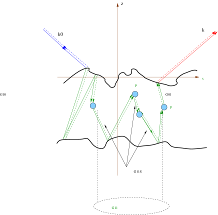
Figure 1: Scattering processes under the ladder approximation. The solid line and the dashed line represent, respectively, the wave on the left and right hand side of tensorial products such as $\overline{\boldsymbol{\mathcal{G}}}^{11}_{\ll SV\gg}=\scriptstyle\ll\overline{\boldsymbol{G}}^{11}_{SV}\otimes\overline{\boldsymbol{G}}^{11\,*}_{SV}\gg_{SV}$.

As shown in Figure 2, we can also use Feynman diagrams [9, 24, 56] to represent the different terms of $\overline{\boldsymbol{\mathcal{G}}}^{11}_{\ll SV\gg}$ in the ladder approximation obtained by iteration of the Bethe-Salpeter equation (111):

$$\overline{\boldsymbol{\mathcal{G}}}^{11}_{\ll SV\gg}=\overline{\boldsymbol{\mathcal{G}}}^{11}_{\infty\,<S>}+\overline{\boldsymbol{\mathcal{G}}}^{11}_{\infty\,<S>}:\overline{\boldsymbol{\mathcal{P}}}^{11}:\overline{\boldsymbol{\mathcal{G}}}^{11}_{\infty\,<S>}$$

$$\hbox to0.0pt{\hss${}+{}$}\overline{\boldsymbol{\mathcal{G}}}^{11}_{\infty\,<S>}:\overline{\boldsymbol{\mathcal{P}}}^{11}:\overline{\boldsymbol{\mathcal{G}}}^{11}_{\infty\,<S>}:\overline{\boldsymbol{\mathcal{P}}}^{11}:\overline{\boldsymbol{\mathcal{G}}}^{11}_{\infty\,<S>}+\dots\,.$$ (120)

Figure 2: Diagrammatic representation of the ladder approximation.

We now examine in detail the different terms in the Bethe-Salpeter equation (111). Since, by hypothesis, the medium and the surfaces are statistically homogeneous, we introduce a Fourier transform along the $X$, $Y$ axis:

$$\overline{\boldsymbol{\mathcal{G}}}(Z,\boldsymbol{k}|Z_{0},\boldsymbol{k}_{0};\boldsymbol{P})=\int\rmd^{2}(\boldsymbol{X}-\boldsymbol{X}_{0})\,\,\rme^{-\rmi(\boldsymbol{X}-\boldsymbol{X}_{0})\cdot\boldsymbol{P}}\,\,\overline{\boldsymbol{\mathcal{G}}}(\boldsymbol{R},\boldsymbol{k}|\boldsymbol{R}_{0},\boldsymbol{k}_{0})\,,$$ (121)

with

$$\boldsymbol{R}=X\hat{\boldsymbol{e}}_{x}+Y\hat{\boldsymbol{e}}_{y}+Z\hat{\boldsymbol{e}}_{z}=\boldsymbol{X}+Z\hat{\boldsymbol{e}}_{z}\,,$$ (122)

$$\boldsymbol{R}_{0}=X_{0}\hat{\boldsymbol{e}}_{x}+Y_{0}\hat{\boldsymbol{e}}_{y}+Z_{0}\hat{\boldsymbol{e}}_{z}=\boldsymbol{X}_{0}+Z_{0}\hat{\boldsymbol{e}}_{z}\,,$$ (123)

and where $\overline{\boldsymbol{\mathcal{G}}}$ is either $\overline{\boldsymbol{\mathcal{G}}}^{11}_{\ll SV\gg}$, $\overline{\boldsymbol{\mathcal{G}}}^{11}_{\infty\,<S>}$, $\overline{\boldsymbol{\mathcal{G}}}^{1a1a_{0}}_{<S>}$, or $\overline{\boldsymbol{\mathcal{G}}}^{11}_{\infty}$. With this Fourier transform, equation (114) is now

$$\overline{\boldsymbol{\mathcal{G}}}^{11}_{\infty\,<S>}(Z,\boldsymbol{k}|Z_{0},\boldsymbol{k}_{0};\boldsymbol{P})=\overline{\boldsymbol{\mathcal{G}}}_{\infty}^{11}(Z,\boldsymbol{k}|Z_{0},\boldsymbol{k}_{0};\boldsymbol{P})+\sum_{a,a_{0}=\pm}\,\overline{\boldsymbol{\mathcal{G}}}^{1a1a_{0}}_{<S>}(Z,\boldsymbol{k}|Z_{0},\boldsymbol{k}_{0};\boldsymbol{P})\,.$$ (124)

Furthermore, in calculating the terms $\overline{\boldsymbol{\mathcal{G}}}^{1a1a_{0}}_{<S>}$ and $\overline{\boldsymbol{\mathcal{G}}}^{\infty}_{1}$ in equation (124) and using the Weyl representation of $\overline{\boldsymbol{G}}^{\infty}_{1}$ and the Green function decomposition in terms of the scattering operator $\overline{\boldsymbol{S}}^{1a1a_{0}}$ given in I and mentioned at the end of section (3), we obtain the following decomposition:

$$\overline{\boldsymbol{\mathcal{G}}}^{1a1a_{0}}_{<S>}(Z,\boldsymbol{k}|Z_{0},\boldsymbol{k}_{0};\boldsymbol{P})=(2\pi)^{2}\,\delta\left(k_{z}-a\,\frac{\alpha_{e}(\boldsymbol{p}^{+})+\alpha^{*}_{e}(\boldsymbol{p}^{-})}{2}\right)$$

$$\hbox to0.0pt{\hss${}\times{}$}\delta\left(k_{0z}-a_{0}\,\frac{\alpha_{e}(\boldsymbol{p}_{0}^{+})+\alpha^{*}_{e}(\boldsymbol{p}_{0}^{-})}{2}\right)\,\overline{\boldsymbol{\mathcal{G}}}^{1a1a_{0}}_{<S>}(Z,\boldsymbol{p}|Z_{0},\boldsymbol{p}_{0};\boldsymbol{P})\,,$$ (125)

$$\overline{\boldsymbol{\mathcal{G}}}^{11}_{\infty}(Z,\boldsymbol{k}|Z_{0},\boldsymbol{k}_{0};\boldsymbol{P})=\sum_{a,a_{0}=\pm}(2\pi)^{2}\,\delta\left(k_{z}-a\,\frac{\alpha_{e}(\boldsymbol{p}^{+})+\alpha^{*}_{e}(\boldsymbol{p}^{-})}{2}\right)$$

$$\hbox to0.0pt{\hss${}\times{}$}\delta\left(k_{0z}-a_{0}\,\frac{\alpha_{e}(\boldsymbol{p}_{0}^{+})+\alpha^{*}_{e}(\boldsymbol{p}_{0}^{-})}{2}\right)\,\overline{\boldsymbol{\mathcal{G}}}^{1a1a_{0}}_{\infty}(Z,\boldsymbol{p}|Z_{0},\boldsymbol{p}_{0};\boldsymbol{P})\,,$$

(126)

where $a$ and $a_{0}$ are the signs $+$ or $-$, $\boldsymbol{k}=\boldsymbol{p}+k_{z}\,\hat{\boldsymbol{e}}_{z}$, $\boldsymbol{k}_{0}=\boldsymbol{p}_{0}+k_{0z}\,\hat{\boldsymbol{e}}_{z}$, and

$$\boldsymbol{p}^{\pm}=\boldsymbol{p}\pm\frac{\boldsymbol{P}}{2}\,,\qquad\boldsymbol{p}_{0}^{\pm}=\boldsymbol{p}_{0}\pm\frac{\boldsymbol{P}}{2}\,.$$ (127)

Under the quasi-uniform field approximation [13], we approximate $\alpha_{e}(\boldsymbol{p}_{0}^{+})+\alpha^{*}_{e}(\boldsymbol{p}_{0}^{-})$ by $\alpha_{e}(\boldsymbol{p})+\alpha^{*}_{e}(\boldsymbol{p})=2\mathrm{Re}\,\alpha_{e}(\boldsymbol{p})$, and equations (125) and (126) become

$$\overline{\boldsymbol{\mathcal{G}}}^{1a1a_{0}}_{<S>}(Z,\boldsymbol{k}|Z_{0},\boldsymbol{k}_{0};\boldsymbol{P})$$

$$\hbox to0.0pt{\hss${}={}$}(2\pi)^{2}\delta(k_{z}-a\,\alpha^{\prime}_{e}(\boldsymbol{p}))\,\delta(k_{0z}-a_{0}\,\alpha^{\prime}_{e}(\boldsymbol{p}_{0}))\,\overline{\boldsymbol{\mathcal{G}}}^{1a1a_{0}}_{<S>}(Z,\boldsymbol{p}|Z_{0},\boldsymbol{p}_{0};\boldsymbol{P})\,,$$ (128)

$$\overline{\boldsymbol{\mathcal{G}}}^{11}_{\infty}(Z,\boldsymbol{k}|Z_{0},\boldsymbol{k}_{0};\boldsymbol{P})$$

$$\hbox to0.0pt{\hss${}={}$}\!\!\sum_{a,a_{0}=\pm}\!\!(2\pi)^{2}\delta(k_{z}-a\,\alpha^{\prime}_{e}(\boldsymbol{p}))\,\delta(k_{0z}-a_{0}\,\alpha^{\prime}_{e}(\boldsymbol{p}_{0}))\,\overline{\boldsymbol{\mathcal{G}}}^{1a1a_{0}}_{\infty}(Z,\boldsymbol{p}|Z_{0},\boldsymbol{p}_{0};\boldsymbol{P})\,,$$

$$\,,$$ (129)

where $\alpha^{\prime}_{e}(\boldsymbol{p})=\mathrm{Re}[\alpha_{e}(\boldsymbol{p})]$. The Dirac distributions insure that the wave vector directions $\boldsymbol{k}$ and $\boldsymbol{k}_{0}$ have constant norms $||\boldsymbol{k}||\simeq K_{e}^{\prime}$, $||\boldsymbol{k}_{0}||\simeq K_{e}^{\prime}$. Furthermore, we found the following expression for the tensors $\overline{\boldsymbol{\mathcal{G}}}^{1a1a_{0}}_{<S>}$ and $\overline{\boldsymbol{\mathcal{G}}}^{1a1a_{0}}_{\infty}$:

$$\overline{\boldsymbol{\mathcal{G}}}^{1a1a_{0}}_{<S>}(Z,\boldsymbol{p}|Z_{0},\boldsymbol{p}_{0};\boldsymbol{P}) =\overline{\boldsymbol{\mathcal{S}}}^{1a1a_{0}}_{\otimes\,<S>}(\boldsymbol{p}|\boldsymbol{p}_{0};\boldsymbol{P})\frac{\rme^{\rmi\,a\,\Delta\alpha(\boldsymbol{p};\boldsymbol{P})\,Z-\rmi\,a_{0}\,\Delta\alpha(\boldsymbol{p}_{0};\boldsymbol{P})\,Z_{0}}}{4\,\alpha_{e}(\boldsymbol{p}_{0}^{+})\alpha_{e}^{*}(\boldsymbol{p}_{0}^{-})}\,\,,$$ (130)

$$\overline{\boldsymbol{\mathcal{G}}}^{1a1a_{0}}_{\infty}(Z,\boldsymbol{p}|Z_{0},\boldsymbol{p}_{0};\boldsymbol{P}) =(2\pi)^{2}\,\delta(\boldsymbol{p}-\boldsymbol{p}_{0})\overline{\boldsymbol{I}}_{\perp}^{1a}(\boldsymbol{p}^{+})\otimes\overline{\boldsymbol{I}}_{\perp}^{1a\,*}(\boldsymbol{p}^{-})\,\delta_{a,a_{0}}\,\delta_{a,sgn(Z-Z_{0})}\$$ (131)

$$\times\frac{\,\rme^{\rmi\,a\,\Delta\alpha_{e}(\boldsymbol{p};\boldsymbol{P})\,(Z-Z_{0})}}{4\,\alpha_{e}(\boldsymbol{p}^{+})\alpha_{e}^{*}(\boldsymbol{p}^{-})}\,,$$

where

$$\delta_{a,\mathrm{sgn}(Z-Z_{0})}=\left\{\begin{array}[]{ll}1&\mbox{if }a=\mathrm{sgn}(Z-Z_{0})\\ 0&\mbox{if }a\neq\mathrm{sgn}(Z-Z_{0})\,,\end{array}\right.$$ (132)

with $\mathrm{sgn}(Z-Z_{0})$ the sign of $Z-Z_{0}$, and

$$\Delta\alpha_{e}(\boldsymbol{p};\boldsymbol{P})=\alpha_{e}(\boldsymbol{p}^{+})-\alpha^{*}_{e}(\boldsymbol{p}^{-})\,,$$ (133)

$$\overline{\boldsymbol{I}}_{\perp}^{1a}(\boldsymbol{p})=(\overline{\boldsymbol{I}}-\hat{\boldsymbol{k}}^{1a}_{\boldsymbol{p}}\hat{\boldsymbol{k}}^{1a}_{\boldsymbol{p}})=\hat{\boldsymbol{e}}_{V}^{1a}(\boldsymbol{p})\hat{\boldsymbol{e}}_{V}^{1a}(\boldsymbol{p})+\hat{\boldsymbol{e}}_{H}(\boldsymbol{p})\hat{\boldsymbol{e}}_{H}(\boldsymbol{p})\,,$$ (134)

$$\boldsymbol{k}^{1a}_{\boldsymbol{p}}=\boldsymbol{p}+a\,\alpha_{e}(\boldsymbol{p})\,\hat{\boldsymbol{e}}_{z}\,,\quad\hat{\boldsymbol{k}}^{1a}_{\boldsymbol{p}}=\boldsymbol{k}^{1a}_{\boldsymbol{p}}/||\boldsymbol{k}^{1a}_{\boldsymbol{p}}||\,.$$ (135)

The tensors $\overline{\boldsymbol{\mathcal{S}}}_{\otimes\,<S>}^{1a\,1a_{0}}$ describe the intensity scattered by the boundaries and are defined by

$$(2\pi)^{2}\,\delta(\boldsymbol{0})\,\overline{\boldsymbol{\mathcal{S}}}_{\otimes\,<S>}^{1a\,1a_{0}}(\boldsymbol{p}|\boldsymbol{p}_{0};\boldsymbol{P}_{0})=<\overline{\boldsymbol{S}}^{1a1a_{0}}\left(\boldsymbol{p}^{+}|\boldsymbol{p}_{0}^{+}\right)\otimes\overline{\boldsymbol{S}}^{1a\,1a_{0}\,*}\left(\boldsymbol{p}^{-}|\boldsymbol{p}_{0}^{-}\right)>_{S}\,.$$ (136)

In introducing properties (128) and (129) in the Bethe-Salpeter equation (111), we demonstrate that $\overline{\boldsymbol{\mathcal{G}}}^{11}_{\ll SV\gg}$ verifies a development similar to equations (128) and (129):

$$\overline{\boldsymbol{\mathcal{G}}}^{11}_{\ll SV\gg}(Z,\boldsymbol{p}|Z_{0},\boldsymbol{p}_{0};\boldsymbol{P})$$

$$=\sum_{a,a_{0}=\pm}(2\pi)^{2}\delta(k_{z}-a\,\alpha^{\prime}_{e}(\boldsymbol{p}))\,\delta(k_{0z}-a_{0}\,\alpha^{\prime}_{e}(\boldsymbol{p}_{0}))\,\overline{\boldsymbol{\mathcal{G}}}^{1a1a_{0}}_{\ll SV\gg}(Z,\boldsymbol{p}|Z_{0},\boldsymbol{p}_{0};\boldsymbol{P})\,.$$ (137)

Accordingly, we can write equation (111) for each sign $a$ and $a_{0}$, and we have

$$\overline{\boldsymbol{\mathcal{G}}}^{1a1a_{0}}_{\ll SV\gg}(Z,\hat{\boldsymbol{k}}|Z_{0},\hat{\boldsymbol{k}}_{0};\boldsymbol{P})=\overline{\boldsymbol{\mathcal{G}}}^{1a1a_{0}}_{\infty<S>}(Z,\boldsymbol{p}|Z_{0},\boldsymbol{p}_{0};\boldsymbol{P})+\sum_{a_{1},a_{2}}\,\int\frac{\rmd^{2}\boldsymbol{p}_{1}}{(2\pi)^{2}}\frac{\rmd^{2}\boldsymbol{p}_{2}}{(2\pi)^{2}}\int_{-H}^{0}\rmd Z_{21}\,\,$$

$$\times\overline{\boldsymbol{\mathcal{G}}}^{1a1a_{2}}_{\infty<S>}(Z,\boldsymbol{p}|Z_{21},\boldsymbol{p}_{2};\boldsymbol{P}):\overline{\boldsymbol{\mathcal{P}}}^{1a_{2}1a_{1}}(\boldsymbol{p}_{2}|\boldsymbol{p}_{1};\boldsymbol{P}):\overline{\boldsymbol{\mathcal{G}}}^{1a_{1}a_{0}}_{\ll SV\gg}(Z_{21},\boldsymbol{p}_{1}|Z_{0},\boldsymbol{p}_{0};\boldsymbol{P})\,,$$ (138)

with

$$\overline{\boldsymbol{\mathcal{G}}}^{1a1a_{0}}_{\infty<S>}(Z,\boldsymbol{p}|Z_{0},\boldsymbol{p}_{0};\boldsymbol{P})=\overline{\boldsymbol{\mathcal{G}}}^{1a1a_{0}}_{\infty}(Z,\boldsymbol{p}|Z_{0},\boldsymbol{p}_{0};\boldsymbol{P})+\overline{\boldsymbol{\mathcal{G}}}^{1a1a_{0}}_{<S>}(Z,\boldsymbol{p}|Z_{0},\boldsymbol{p}_{0};\boldsymbol{P})\,,$$ (139)

$$\overline{\boldsymbol{\mathcal{P}}}^{1a_{2}1a_{1}}(\boldsymbol{p}_{2}|\boldsymbol{p}_{1};\boldsymbol{P})=n\,w(\hat{\boldsymbol{k}}^{1a_{2}}_{\boldsymbol{p}_{2}}-\hat{\boldsymbol{k}}^{1a_{1}}_{\boldsymbol{p}_{1}})\,\overline{\boldsymbol{C}}^{11}_{o}(\hat{\boldsymbol{k}}^{1a_{2}}_{\boldsymbol{p}_{2}^{+}}|\hat{\boldsymbol{k}}^{1a_{1}}_{\boldsymbol{p}_{1}^{+}})\otimes\overline{\boldsymbol{C}}^{11\,*}_{o}(\hat{\boldsymbol{k}}^{1a_{2}}_{\boldsymbol{p}_{2}^{-}}|\hat{\boldsymbol{k}}^{1a_{1}}_{\boldsymbol{p}_{1}^{-}})\ \,$$ (140)

$$\boldsymbol{p}_{1}^{\pm}=\boldsymbol{p}_{1}\pm\frac{\boldsymbol{P}}{2}\,,\qquad\boldsymbol{p}_{2}^{\pm}=\boldsymbol{p}_{2}\pm\frac{\boldsymbol{P}}{2}\,,$$ (141)

$$\hat{\boldsymbol{k}}^{1a}_{\boldsymbol{p}}=\boldsymbol{p}+a\,\alpha^{\prime}_{e}(\boldsymbol{p})\,\hat{\boldsymbol{e}}_{z}\,.$$ (142)

The numerical solution of integral equation (138) is a difficult task, and in the next section, we will give a differential form of this equation more appropriate in this case. However, equation (138) is well suited if we want to obtain an iterative solution for $\overline{\boldsymbol{\mathcal{G}}}^{1a1a_{0}}_{\ll SV\gg}$. For example, in introducing the first term of this iteration,

$$\overline{\boldsymbol{\mathcal{G}}}^{1a1a_{0}}_{\infty<S>}(Z,\boldsymbol{p}|Z_{0},\boldsymbol{p}_{0};\boldsymbol{P})=\overline{\boldsymbol{\mathcal{G}}}^{1a1a_{0}}_{\infty}(Z,\boldsymbol{p}|Z_{0},\boldsymbol{p}_{0};\boldsymbol{P})+\overline{\boldsymbol{\mathcal{G}}}^{1a1a_{0}}_{<S>}(Z,\boldsymbol{p}|Z_{0},\boldsymbol{p}_{0};\boldsymbol{P})$$

in equation (81), we obtain the double scattering contribution by the particles. The term $\overline{\boldsymbol{\mathcal{G}}}^{\infty\,aa_{0}}_{1}$ describes the direct propagation of the wave between the two scatterers, and $\overline{\boldsymbol{\mathcal{G}}}^{1a1a_{0}}_{<S>}$ describes the interaction with the boundaries between the two scattering processes by the particles.

6 Radiative transfer equation and boundaries conditions

To derive the radiative transfer equation verified by $\overline{\boldsymbol{\mathcal{G}}}^{1a1a_{0}}_{\ll SV\gg}(Z,\boldsymbol{p}|Z_{0},\boldsymbol{p}_{0};\boldsymbol{P})$, we must first notice the following properties of $\overline{\boldsymbol{\mathcal{G}}}_{\infty}^{1a1a_{0}}$ and $\overline{\boldsymbol{\mathcal{G}}}^{1a1a_{0}}_{<S>}$:

$$\frac{\partial}{\partial\scriptstyle{Z}}\overline{\boldsymbol{\mathcal{G}}}^{1a1a_{0}}_{\infty}(Z,\boldsymbol{p}|Z_{0},\boldsymbol{p}_{0};\boldsymbol{P}) =\frac{(2\pi)^{2}\,\delta(\boldsymbol{p}-\boldsymbol{p}_{0})}{4\,\alpha_{e}(\boldsymbol{p}^{+})\alpha_{e}^{*}(\boldsymbol{p}^{-})}\,\overline{\boldsymbol{I}}_{\perp\,\otimes}^{1\,a}(\boldsymbol{p};\boldsymbol{P})\,\delta_{a,a_{0}}\,a\,\delta(Z-Z_{0})\,,$$ (143)

$$+\rmi\,a\,\Delta\alpha_{e}(\boldsymbol{p};\boldsymbol{P})\,\overline{\boldsymbol{\mathcal{G}}}^{1a1a_{0}}_{\infty}(Z,\boldsymbol{p}|Z_{0},\boldsymbol{p}_{0};\boldsymbol{P})$$

$$\frac{\partial}{\partial\scriptstyle{Z}}\overline{\boldsymbol{\mathcal{G}}}^{1a1a_{0}}_{<S>}(Z,\boldsymbol{p}|Z_{0},\boldsymbol{p}_{0};\boldsymbol{P}) =\rmi\,a\,\Delta\alpha_{e}(\boldsymbol{p};\boldsymbol{P})\,\overline{\boldsymbol{\mathcal{G}}}^{1a1a_{0}}_{<S>}(Z,\boldsymbol{p}|Z_{0},\boldsymbol{p}_{0};\boldsymbol{P})\,,$$ (144)

with

$$\overline{\boldsymbol{I}}^{1a}_{\perp\,\otimes}(\boldsymbol{p};\boldsymbol{P})=\overline{\boldsymbol{I}}_{\perp}^{1a}(\boldsymbol{p}^{+})\otimes\overline{\boldsymbol{I}}_{\perp}^{1a\,*}(\boldsymbol{p}^{-})\,.$$ (145)

$$\boldsymbol{p}^{\pm}=\boldsymbol{p}\pm\frac{\boldsymbol{P}}{2}\,.$$ (146)

To obtain equation (143), we have to introduce in equation (131) the identity

$$\hbox to0.0pt{\hss${}\delta{}$}_{a,\mathrm{sgn}(Z-Z_{0})}=\delta_{a,+}\Theta(Z-Z_{0})+\delta_{a,-}\Theta(Z_{0}-Z)\,,$$ (147)

with $\Theta$ as the Heaviside function, and then use the property:

$$\frac{\rmd\Theta}{\rmd z}(z)=\delta(z)\,.$$ (148)

Hence, in taking the derivative of the Bethe-Salpeter equation (138), we obtain the radiative transfer equation satisfied by $\overline{\boldsymbol{\mathcal{G}}}^{1a1a_{0}}_{\ll SV\gg}(Z,\boldsymbol{p}|Z_{0},\boldsymbol{p}_{0};\boldsymbol{P})$ :

$$\frac{\partial}{\partial\scriptstyle{Z}}\overline{\boldsymbol{\mathcal{G}}}^{1a1a_{0}}_{\ll SV\gg}(Z,\boldsymbol{p}|Z_{0},\boldsymbol{p}_{0};\boldsymbol{P})=\frac{(2\pi)^{2}\,\delta(\boldsymbol{p}-\boldsymbol{p}_{0})}{4\,\alpha_{e}(\boldsymbol{p}^{+})\alpha_{e}^{*}(\boldsymbol{p}^{-})}\,\overline{\boldsymbol{I}}_{\perp\,\otimes}^{1\,a}(\boldsymbol{p};\boldsymbol{P})\,\delta_{a,a_{0}}\,a\,\delta({Z-Z_{0}})$$

$$\quad+\frac{a}{4\,\alpha_{e}(\boldsymbol{p}^{+})\alpha_{e}^{*}(\boldsymbol{p}^{-})}\,\sum_{a_{1}=\pm}\int\frac{\rmd^{2}\boldsymbol{p}_{1}}{(2\pi)^{2}}\,\,\overline{\boldsymbol{\mathcal{P}}}^{1a1a_{1}}(\boldsymbol{p}|\boldsymbol{p}_{1};\boldsymbol{P}):\overline{\boldsymbol{\mathcal{G}}}^{1a_{1}a_{0}}_{\ll SV\gg}(Z,\boldsymbol{p}_{1}|Z_{0},\boldsymbol{p}_{0};\boldsymbol{P})$$

$$\quad+\rmi\,a\,\Delta\alpha_{e}(\boldsymbol{p};\boldsymbol{P})\,\overline{\boldsymbol{\mathcal{G}}}^{1a_{1}a_{0}}_{\ll SV\gg}(Z,\boldsymbol{p}|Z_{0},\boldsymbol{p}_{0};\boldsymbol{P})\,.$$ (150)

To solve this differential equation, we need boundary conditions on the interface. In I, we have shown that the scattering operator $\overline{\boldsymbol{S}}^{1\pm 1\pm}$ can be decomposed as a function of the scattering operators $\overline{\boldsymbol{R}}^{01}$ and $\overline{\boldsymbol{R}}^{H\,21}$ of the upper and lower rough surfaces. In using these equations, we easily show the following relationships between the scattering operators:

$$\overline{\boldsymbol{S}}^{1-1-}=\overline{\boldsymbol{R}}^{01}\cdot\overline{\boldsymbol{S}}^{1+1-}\,,$$ (151)

$$\overline{\boldsymbol{S}}^{1-1+}=\overline{\boldsymbol{R}}^{01}+\overline{\boldsymbol{R}}^{01}\cdot\overline{\boldsymbol{S}}^{1+1+}\,,$$ (152)

$$\overline{\boldsymbol{S}}^{1+1-}=\overline{\boldsymbol{R}}^{H\,21}+\overline{\boldsymbol{R}}^{H\,21}\cdot\overline{\boldsymbol{S}}^{1+1-}\,,$$ (153)

$$\overline{\boldsymbol{S}}^{1+1+}=\overline{\boldsymbol{R}}^{H\,21}\cdot\overline{\boldsymbol{S}}^{1-1+}\,.$$ (154)

where we have used the notation,

$$[\overline{\boldsymbol{f}}\cdot\overline{\boldsymbol{g}}](\boldsymbol{p}|\boldsymbol{p}_{0})\equiv\int\frac{\rmd^{2}\boldsymbol{p}_{1}}{(2\pi)^{2}}\,\,\overline{\boldsymbol{f}}(\boldsymbol{p}|\boldsymbol{p}_{1})\cdot\overline{\boldsymbol{g}}(\boldsymbol{p}_{1}|\boldsymbol{p}_{0})\,.$$ (155)

With equations (130,131,151-154) and the definition of $\overline{\boldsymbol{R}}^{H\,21}$ given in I:

$$\overline{\boldsymbol{R}}^{H\,21}(\boldsymbol{p}|\boldsymbol{p}_{0})=\rme^{\rmi\,(\alpha_{1}(\boldsymbol{p})+\alpha_{1}(\boldsymbol{p}_{0}))\,H}\,\overline{\boldsymbol{R}}^{21}(\boldsymbol{p}|\boldsymbol{p}_{0})\,,$$ (156)

we obtain

$$\overline{\boldsymbol{\mathcal{G}}}^{1-1a_{0}}_{\infty<S>}(Z=0,\boldsymbol{p}|Z_{0},\boldsymbol{p}_{0};\boldsymbol{P})$$

$$=\int\frac{\rmd^{2}\boldsymbol{p}_{1}}{(2\pi)^{2}}\,\,\overline{\boldsymbol{\mathcal{R}}}^{01}_{\otimes\,<S>}(\boldsymbol{p}|\boldsymbol{p}_{1};\boldsymbol{P}):\overline{\boldsymbol{\mathcal{G}}}^{1+1a_{0}}_{\infty<S>}(Z=0,\boldsymbol{p}_{1}|Z_{0},\boldsymbol{p}_{0};\boldsymbol{P})\,,$$ (157)

$$\overline{\boldsymbol{\mathcal{G}}}^{1+1a_{0}}_{\infty<S>}(Z=-H,\boldsymbol{p}|Z_{0},\boldsymbol{p}_{0};\boldsymbol{P})$$

$$=\int\frac{\rmd^{2}\boldsymbol{p}_{1}}{(2\pi)^{2}}\,\,\overline{\boldsymbol{\mathcal{R}}}^{21}_{\otimes\,<S>}(\boldsymbol{p}|\boldsymbol{p}_{1};\boldsymbol{P}):\overline{\boldsymbol{\mathcal{G}}}^{1-1a_{0}}_{\infty<S>}(Z=-H,\boldsymbol{p}_{1}|Z_{0},\boldsymbol{p}_{0};\boldsymbol{P})\,,$$ (158)

where we have defined

$$(2\pi)^{2}\,\delta(\boldsymbol{0})\,\overline{\boldsymbol{\mathcal{R}}}^{01}_{\otimes\,<S>}(\boldsymbol{p}|\boldsymbol{p}_{0};\boldsymbol{P}) =<\overline{\boldsymbol{R}}^{01}(\boldsymbol{p}^{+}|\boldsymbol{p}_{0}^{+})\otimes\overline{\boldsymbol{R}}^{01}(\boldsymbol{p}^{-}|\boldsymbol{p}_{0}^{-})>_{S}\,,$$ (159)

$$(2\pi)^{2}\,\delta(\boldsymbol{0})\,\overline{\boldsymbol{\mathcal{R}}}^{21}_{\otimes<S>}(\boldsymbol{p}|\boldsymbol{p}_{0};\boldsymbol{P}) =<\overline{\boldsymbol{R}}^{21}(\boldsymbol{p}^{+}|\boldsymbol{p}_{0}^{+})\otimes\overline{\boldsymbol{R}}^{21}(\boldsymbol{p}^{-}|\boldsymbol{p}_{0}^{-})>_{S}\,.$$ (160)

Then, with the help of the Bethe-Salpeter equation (138), we easily demonstrate that $\overline{\boldsymbol{\mathcal{G}}}^{1a1a_{0}}_{\ll SV\gg}(Z,\boldsymbol{p}|Z_{0},\boldsymbol{p}_{0};\boldsymbol{P})$ verifies the following boundary conditions on the upper and lower rough surfaces:

$$\overline{\boldsymbol{\mathcal{G}}}^{1-1a_{0}}_{\ll SV\gg}(Z=0,\boldsymbol{p}|Z_{0},\boldsymbol{p}_{0};\boldsymbol{P})$$ (161)

$$=\int\frac{\rmd^{2}\boldsymbol{p}_{1}}{(2\pi)^{2}}\,\overline{\boldsymbol{\mathcal{R}}}^{01}_{\otimes\,<S>}(\boldsymbol{p}|\boldsymbol{p}_{1};\boldsymbol{P}):\overline{\boldsymbol{\mathcal{G}}}^{1+1a_{0}}_{\ll SV\gg}(Z=0,\boldsymbol{p}_{1}|Z_{0},\boldsymbol{p}_{0};\boldsymbol{P})\,,$$ (162)

$$\overline{\boldsymbol{\mathcal{G}}}^{1+1a_{0}}_{\ll SV\gg}(Z=-H,\boldsymbol{p}|Z_{0},\boldsymbol{p}_{0};\boldsymbol{P})$$ (163)

$$=\int\frac{\rmd^{2}\boldsymbol{p}_{1}}{(2\pi)^{2}}\,\overline{\boldsymbol{\mathcal{R}}}^{21}_{\otimes\,<S>}(\boldsymbol{p}|\boldsymbol{p}_{1};\boldsymbol{P}):\overline{\boldsymbol{\mathcal{G}}}^{1-1a_{0}}_{\ll SV\gg}(Z=-H,\boldsymbol{p}_{1}|Z_{0},\boldsymbol{p}_{0};\boldsymbol{P})\,,$$ (164)

With equation (150) and the boundary conditions (162), (164) we thus have obtained a closed system of equations sufficient to calculate the tensors $\overline{\boldsymbol{\mathcal{G}}}^{1a1a_{0}}_{\ll SV\gg}$. In section (12), we will show how to rewrite the radiative transfer equation (150) in a more classical form.

7 Calculation of $\overline{\boldsymbol{\sigma}}^{incoh}_{L=0}$

In sections (2) and (3), we have shown that the first term of the incoherent scattering cross-section is given by

$$\frac{\alpha_{0}(\boldsymbol{p})^{2}}{\pi}\,\boldsymbol{\mathcal{I}}^{incoh}_{L=0}(\boldsymbol{R},\boldsymbol{k})=(2\pi)\,\delta(k_{z}-\alpha_{0}(\boldsymbol{p}))\,\overline{\boldsymbol{\sigma}}^{incoh}_{L=0}(\boldsymbol{p}|\boldsymbol{p}_{0}):\boldsymbol{\mathcal{J}}^{0\,i}(\boldsymbol{p}_{0})\,,$$ (165)

with $\boldsymbol{k}=\boldsymbol{p}+k_{z}\hat{\boldsymbol{e}}_{z}$ and

$$\boldsymbol{\mathcal{I}}^{incoh}_{L=0}(\boldsymbol{R},\boldsymbol{k})= e_{0}\int_{V_{0}}\rmd^{3}\boldsymbol{r}\rme^{-\rmi\,\boldsymbol{k}\cdot\boldsymbol{r}}\,\left[<\boldsymbol{E}^{0\,s}_{S}(\boldsymbol{R}+\frac{\boldsymbol{r}}{2})\otimes\boldsymbol{E}^{0\,s\,*}_{S}(\boldsymbol{R}-\frac{\boldsymbol{r}}{2})>_{S}\right.$$ (166)

$$\left.\qquad\qquad\qquad-<\boldsymbol{E}^{0\,s}_{S}(\boldsymbol{R}+\frac{\boldsymbol{r}}{2})>\otimes<\boldsymbol{E}^{0\,s\,*}_{S}(\boldsymbol{R}-\frac{\boldsymbol{r}}{2})>_{S}\right]\,.$$

Furthermore, we know that the scattering intensity $\boldsymbol{E}^{0\,s}_{S}$ can be expressed as a function of the scattering operator $\overline{\boldsymbol{S}}^{0+0-}$ by

$$\boldsymbol{E}^{0s}_{S}(\boldsymbol{x},z)=\int\frac{\rmd^{2}\boldsymbol{p}}{(2\pi)^{2}}\,\,\rme^{\rmi\,\boldsymbol{p}\cdot\boldsymbol{x}+\rmi\,\alpha_{0}(\boldsymbol{p})\,z}\,\overline{\boldsymbol{S}}^{0+,0-}(\boldsymbol{p}|\boldsymbol{p}_{0})\cdot\boldsymbol{E}^{0\,i}(\boldsymbol{p}_{0})\,.$$ (167)

Then, we find

$$\overline{\boldsymbol{\sigma}}^{incoh}_{L=0}(\boldsymbol{p}|\boldsymbol{p}_{0})=\frac{\alpha_{0}(\boldsymbol{p})^{2}}{\pi}\,\overline{\boldsymbol{\mathcal{S}}}^{0+0-incoh}_{\otimes<S>}(\boldsymbol{p}|\boldsymbol{p}_{0})\,,\\$$

where $\overline{\boldsymbol{\mathcal{S}}}^{0+0-incoh}_{\otimes<S>}$ is defined by

$$(2\pi)^{2}\delta(\boldsymbol{0})\,\overline{\boldsymbol{\mathcal{S}}}^{0+0-incoh}_{\otimes<S>}(\boldsymbol{p}|\boldsymbol{p}_{0})= <\overline{\boldsymbol{S}}^{0+0-}(\boldsymbol{p}|\boldsymbol{p}_{0})\otimes\overline{\boldsymbol{S}}^{0+0-}(\boldsymbol{p}|\boldsymbol{p}_{0})>_{S}$$ (168)

$$-<\overline{\boldsymbol{S}}^{0+0-}(\boldsymbol{p}|\boldsymbol{p}_{0})>_{S}\otimes<\overline{\boldsymbol{S}}^{0+0-}(\boldsymbol{p}|\boldsymbol{p}_{0})>_{S}\,.$$

8 Calculation of $\overline{\boldsymbol{\sigma}}^{incoh}_{L=1}$

For the first order scattering contribution by the particles, the scattered specific intensity is

$$\boldsymbol{\mathcal{I}}^{incoh}_{L=1}(\boldsymbol{R},\boldsymbol{k})=e_{0}\,\int_{V_{0}}\rmd^{3}\boldsymbol{r}\rme^{-\rmi\,\boldsymbol{k}\cdot\boldsymbol{r}}\,<\overline{\boldsymbol{G}}^{01}_{S}\otimes\overline{\boldsymbol{G}}^{01\,*}_{S}>_{S}:\overline{\boldsymbol{\mathcal{P}}}^{11}:<\boldsymbol{E}^{1\,t}_{S}\otimes\boldsymbol{E}^{1\,t\,*}_{S}>_{S}\,,$$ (169)

and the cross-section verifies the following equation:

$$\frac{\alpha(\boldsymbol{p})^{2}}{\pi}\,\boldsymbol{\mathcal{I}}^{incoh}_{L=1}(\boldsymbol{R},\boldsymbol{k})=(2\pi)\,\delta(k_{z}-\alpha_{0}(\boldsymbol{p}))\,\overline{\boldsymbol{\sigma}}^{incoh}_{L=1}(\boldsymbol{p}|\boldsymbol{p}_{0}):\boldsymbol{\mathcal{J}}^{0\,i}(\boldsymbol{p}_{0})\,.$$ (170)

In introducing equations (87, 88) and 89,which connect the Green function $\overline{\boldsymbol{G}}^{01}$ and the transmitted field $\boldsymbol{E}^{1t}$ to the scattering operators $\overline{\boldsymbol{S}}^{0+1\pm}$ and $\overline{\boldsymbol{S}}^{1\pm 0-}$, in (169) we obtain

$$\overline{\boldsymbol{\sigma}}^{incoh}_{L=1}(\boldsymbol{p}|\boldsymbol{p}_{0})=\frac{\alpha_{0}(\boldsymbol{p})^{2}}{\pi}\,\!\!\!\!\!\sum_{a_{1},a_{2}=\pm}\int\frac{\rmd^{2}\boldsymbol{p}_{1}}{(2\pi)^{2}}\,\frac{\rmd^{2}\boldsymbol{p}_{2}}{(2\pi)^{2}}\frac{1}{4\,|\alpha_{e}(\boldsymbol{p}_{2})|^{2}}\,\frac{\left(\rme^{\rmi[a_{2}\Delta\alpha_{e}(\boldsymbol{p}_{2})-a_{1}\Delta\alpha_{e}(\boldsymbol{p}_{1})]\,H}-1\right)}{\rmi[a_{2}\Delta\alpha_{e}(\boldsymbol{p}_{2})-a_{1}\Delta\alpha_{e}(\boldsymbol{p}_{1})]}$$

$$\times\overline{\boldsymbol{\mathcal{S}}}^{0+;1a_{2}}_{\otimes\,<S>}(\boldsymbol{p}|\boldsymbol{p}_{2};\boldsymbol{P}=0):\overline{\boldsymbol{\mathcal{P}}}^{1a_{2}1a_{1}}(\boldsymbol{p}_{2}|\boldsymbol{p}_{1};\boldsymbol{P}=\boldsymbol{0}):\overline{\boldsymbol{\mathcal{S}}}^{1a_{1};0-}_{\otimes\,<S>}(\boldsymbol{p}_{1}|\boldsymbol{p}_{0};\boldsymbol{P}=\boldsymbol{0})\,,$$ (171)

where

$$(2\pi)^{2}\,\delta(\boldsymbol{0})\,\overline{\boldsymbol{\mathcal{S}}}_{\otimes\,<S>}^{0+;1a_{1}}(\boldsymbol{p}|\boldsymbol{p}_{0};\boldsymbol{P}_{0})=<\overline{\boldsymbol{S}}^{0+1a_{1}}\left(\boldsymbol{p}^{+}|\boldsymbol{p}_{0}^{+}\right)\otimes\overline{\boldsymbol{S}}^{0+1a_{1}}\left(\boldsymbol{p}^{-}|\boldsymbol{p}_{0}^{-}\right)>_{S}\,,$$ (172)

$$(2\pi)^{2}\,\delta(\boldsymbol{0})\overline{\boldsymbol{\mathcal{S}}}_{\otimes\,<S>}^{1a_{2};0-}(\boldsymbol{p}|\boldsymbol{p}_{0};\boldsymbol{P}_{0})=<\overline{\boldsymbol{S}}^{1a_{2}\,0-}\left(\boldsymbol{p}^{+}|\boldsymbol{p}_{0}^{+}\right)\otimes\overline{\boldsymbol{S}}^{1a_{2}\,0-}\left(\boldsymbol{p}^{-}|\boldsymbol{p}_{0}^{-}\right)>_{S}\,,$$ (173)

$$\overline{\boldsymbol{\mathcal{P}}}^{1a_{1}1a_{2}}(\boldsymbol{p}_{2}|\boldsymbol{p}_{1})=n\,w(\boldsymbol{k}^{1a_{2}}_{\boldsymbol{p}_{2}}-\boldsymbol{k}^{1a_{1}}_{\boldsymbol{p}_{1}})\,\overline{\boldsymbol{C}}^{11}_{o}(\boldsymbol{k}^{1a_{2}}_{\boldsymbol{p}_{2}^{+}}|\boldsymbol{k}^{1a_{1}}_{\boldsymbol{p}_{1}^{+}})\otimes\overline{\boldsymbol{C}}^{11}_{o}(\boldsymbol{k}^{1a_{2}}_{\boldsymbol{p}_{2}^{-}}|\boldsymbol{k}^{1a_{1}}_{\boldsymbol{p}_{1}^{-}})\,,$$ (174)

with

$$\boldsymbol{p}^{\pm}=\boldsymbol{p}\pm\frac{\boldsymbol{P}}{2}\,,\quad\boldsymbol{p}_{2}^{\pm}=\boldsymbol{p}_{2}\pm\frac{\boldsymbol{P}}{2}\,,\quad\boldsymbol{p}_{1}^{\pm}=\boldsymbol{p}_{1}\pm\frac{\boldsymbol{P}}{2}\,,\quad\boldsymbol{p}_{0}^{\pm}=\boldsymbol{p}_{0}\pm\frac{\boldsymbol{P}}{2}\,,$$ (175)

$$\boldsymbol{k}^{1a}_{\boldsymbol{p}}=p{}+a\,\alpha^{\prime}_{e}(\boldsymbol{p})\,\hat{\boldsymbol{e}}_{z}\,,$$ (176)

and

$$\Delta\alpha_{e}(\boldsymbol{p}) =\alpha_{e}(\boldsymbol{p})-[\alpha_{e}(\boldsymbol{p})]^{*}\,$$ (177)

$$=2\rmi\,\mathrm{Im}[\alpha_{e}(\boldsymbol{p})].$$ (178)

9 Calculation of $\overline{\boldsymbol{\sigma}}^{incoh}_{Ladder}$

Similarly to the previous section, the multiple scattering contribution is given by

$$\boldsymbol{\mathcal{I}}^{incoh}_{Ladder}(\boldsymbol{R},\boldsymbol{k})=e_{0}\,\int_{V_{0}}\rmd^{3}\boldsymbol{r}\,\rme^{-\rmi\,\boldsymbol{k}\cdot\boldsymbol{r}}\,<\overline{\boldsymbol{G}}^{01}_{S}\otimes\overline{\boldsymbol{G}}^{01\,*}_{S}>_{S}:\overline{\boldsymbol{\mathcal{P}}}^{11}:\overline{\boldsymbol{\mathcal{G}}}^{11}_{\ll SV\gg}$$

$$\hbox to0.0pt{\hss${}:{}$}\overline{\boldsymbol{\mathcal{P}}}^{11}:<\boldsymbol{E}^{1\,t}_{S}\otimes\boldsymbol{E}^{1\,t\,*}_{S}>_{S}\,,$$ (179)

and the cross-section is

$$\frac{\alpha(\boldsymbol{p})^{2}}{\pi}\,\boldsymbol{\mathcal{I}}^{incoh}_{Ladder}(\boldsymbol{R},\boldsymbol{k})=(2\pi)\,\delta(k_{z}-\alpha_{0}(\boldsymbol{p}))\,\overline{\boldsymbol{\sigma}}^{incoh}_{Ladder}(\boldsymbol{p}|\boldsymbol{p}_{0}):\boldsymbol{\mathcal{J}}^{0\,i}(\boldsymbol{p}_{0})\,.$$ (180)

From equations (87, 88, 89) and properties (121, 137) of the tensor $\overline{\boldsymbol{\mathcal{G}}}^{1a1a_{0}}_{\ll SV\gg}$, we find

$$\overline{\boldsymbol{\sigma}}^{incoh}_{Ladder}(\boldsymbol{p}|\boldsymbol{p}_{0})=\frac{\alpha(\boldsymbol{p})^{2}}{\pi}\,\!\!\!\!\!\sum_{a_{1},a_{2},a_{3},a_{4}=\pm}\int_{-H}^{0}\,\rmd Z_{43}\,\rmd Z_{21}\int\frac{\rmd^{2}\boldsymbol{p}_{1}}{(2\pi)^{2}}\,\frac{\rmd^{2}\boldsymbol{p}_{2}}{(2\pi)^{2}}\,\frac{\rmd^{2}\boldsymbol{p}_{3}}{(2\pi)^{2}}\frac{\rmd^{2}\boldsymbol{p}_{4}}{(2\pi)^{2}}$$

$$\frac{\rme^{-\rmi\,a_{4}\,\Delta\alpha_{e}(\boldsymbol{p}_{4})\,Z_{43}+\rmi\,a_{1}\,\Delta\alpha_{e}(\boldsymbol{p}_{1})\,Z_{21}}}{4\,|\alpha_{e}(\boldsymbol{p}_{4})|^{2}}\overline{\boldsymbol{\mathcal{S}}}_{\otimes\,<S>}^{0+\,1a_{4}}(\boldsymbol{p}|\boldsymbol{p}_{4};\boldsymbol{P}=\boldsymbol{0}):\overline{\boldsymbol{\mathcal{P}}}^{1a_{4}1a_{3}}(\boldsymbol{p}_{4}|\boldsymbol{p}_{3};\boldsymbol{P}=\boldsymbol{0})$$

$$\times\overline{\boldsymbol{\mathcal{G}}}^{1a_{3}1a_{2}}_{\ll SV\gg}(Z_{43},\boldsymbol{p}_{3}|Z_{21},\boldsymbol{p}_{2};\boldsymbol{P}=0):\overline{\boldsymbol{\mathcal{P}}}^{1a_{2}1a_{1}}(\boldsymbol{p}_{2}|\boldsymbol{p}_{1};\boldsymbol{P}=\boldsymbol{0}):\overline{\boldsymbol{\mathcal{S}}}_{\otimes\,<S>}^{1a_{1}\,0-}(\boldsymbol{p}_{1}|\boldsymbol{p}_{0};\boldsymbol{P}=0)\,.$$

(181)

10 Enhanced backscattering and reciprocity

During the last decade, several studies have been concerned with the enhanced backscattering  [9, 13, 24, 25, 26, 27, 30, 31, 57, 58, 59, 60, 61, 62]. This phenomenon produces a peak in the backscattering direction ($\hat{\boldsymbol{k}}=-\hat{\boldsymbol{k}}_{0}$) due to the interference of waves following the same path but in opposite directions (Figure (3)).

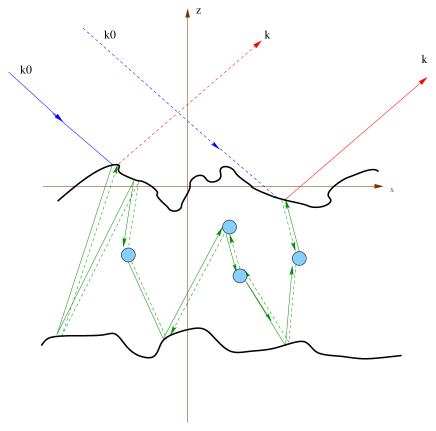
Figure 3: Scattering processes which are taken into account by the most-crossed contribution.

The most elegant way to introduce the enhanced backscattering in the theory is to use the reciprocity principle [63, 64]. Heuristically, it means that when we exchange the source and the detector position (respectively given by $\boldsymbol{r}_{0}$ and $\boldsymbol{r}$) and also their polarization, the field measured is the same. In using our Green functions, we translate this statement by

$$\overline{\boldsymbol{G}}^{00}_{SV}(\boldsymbol{r},\boldsymbol{r}_{0})=[\overline{\boldsymbol{G}}^{00}_{SV}(\boldsymbol{r}_{0},\boldsymbol{r})]^{T}\,,$$ (182)

where the transpose of dyad $\overline{\boldsymbol{f}}$, which exchanges the polarization, is defined by $\overline{\boldsymbol{f}}^{T}\cdot\boldsymbol{E}=\boldsymbol{E}\cdot\overline{\boldsymbol{f}}$. If we decompose the dyad $\overline{\boldsymbol{G}}^{00}_{SV}(\boldsymbol{r},\boldsymbol{r}_{0})$ in the fixed basis $[\hat{\boldsymbol{e}}_{x},\hat{\boldsymbol{e}}_{y},\hat{\boldsymbol{e}}_{z}]$,

$$\overline{\boldsymbol{G}}^{00}_{SV}(\boldsymbol{r},\boldsymbol{r}_{0})=\sum_{i,j=x,y,z}\,{G}^{00}_{SV}(\boldsymbol{r},\boldsymbol{r}_{0})_{ij}\,\hat{\boldsymbol{e}}_{i}\hat{\boldsymbol{e}}_{j}\,,$$ (183)

we re-write equation (182) under the following form:

$${G}^{00}_{SV}(\boldsymbol{r},\boldsymbol{r}_{0})_{ij}={G}^{00}_{SV}(\boldsymbol{r}_{0},\boldsymbol{r})_{ji}\,.$$ (184)

The properties in (182) can be demonstrated by using the Green theorem [65]. By applying these properties on each element of the tensor,

$$\overline{\boldsymbol{\mathcal{G}}}^{00}_{\ll SV\gg}(\boldsymbol{r},\boldsymbol{r}^{\prime}|\boldsymbol{r}_{0},\boldsymbol{r}_{0}^{\prime})=\ll\overline{\boldsymbol{G}}^{00}_{SV}(\boldsymbol{r},\boldsymbol{r}_{0})\otimes\overline{\boldsymbol{G}}^{00\,*}_{SV}(\boldsymbol{r}^{\prime},\boldsymbol{r}_{0}^{\prime})\gg_{SV}\,,$$

we obtain three identities that must be satisfied:

$$\overline{\boldsymbol{G}}^{00}_{SV}\otimes\overline{\boldsymbol{G}}^{00\,*}_{SV}(\boldsymbol{r},\boldsymbol{r}^{\prime}|\boldsymbol{r}_{0},\boldsymbol{r}_{0}^{\prime})=[\overline{\boldsymbol{G}}^{00}_{SV}\otimes\overline{\boldsymbol{G}}^{00\,*}_{SV}(\boldsymbol{r}_{0},\boldsymbol{r}_{0}^{\prime}|\boldsymbol{r},\boldsymbol{r}^{\prime})]^{T_{LR}}\,,$$ (185)

$$\overline{\boldsymbol{G}}^{00}_{SV}\otimes\overline{\boldsymbol{G}}^{00\,*}_{SV}(\boldsymbol{r},\boldsymbol{r}^{\prime}|\boldsymbol{r}_{0},\boldsymbol{r}_{0}^{\prime})=[\overline{\boldsymbol{G}}^{00}_{SV}\otimes\overline{\boldsymbol{G}}^{00\,*}_{SV}(\boldsymbol{r},\boldsymbol{r}_{0}^{\prime}|\boldsymbol{r}_{0},\boldsymbol{r}^{\prime})]^{T_{R}}\,,$$ (186)

$$\overline{\boldsymbol{G}}^{00}_{SV}\otimes\overline{\boldsymbol{G}}^{00\,*}_{SV}(\boldsymbol{r},\boldsymbol{r}^{\prime}|\boldsymbol{r}_{0},\boldsymbol{r}_{0}^{\prime})=[\overline{\boldsymbol{G}}^{00}_{SV}\otimes\overline{\boldsymbol{G}}^{00\,*}_{SV}(\boldsymbol{r}_{0},\boldsymbol{r}^{\prime}|\boldsymbol{r},\boldsymbol{r}^{\prime}_{0})]^{T_{L}}\,,$$ (187)

where we have defined three transposes of a tensor $\overline{\boldsymbol{\mathcal{M}}}$ with the following decomposition (see A):

$$\overline{\boldsymbol{\mathcal{M}}}=\sum_{i,j,i^{\prime},j^{\prime}=x,y,z}\,\mathcal{M}_{ii^{\prime};jj^{\prime}}\left(\hat{\boldsymbol{e}}_{i}\otimes\hat{\boldsymbol{e}}_{i^{\prime}}\right)\left(\hat{\boldsymbol{e}}_{j}\otimes\hat{\boldsymbol{e}}_{j^{\prime}}\right)\,,$$

by

$$\hbox to0.0pt{\hss${}[{}$}\mathcal{M}_{ii^{\prime};jj^{\prime}}]^{T_{LR}}=\mathcal{M}_{jj^{\prime};ii^{\prime}}\,,$$ (188)

$$\hbox to0.0pt{\hss${}[{}$}\mathcal{M}_{ii^{\prime};jj^{\prime}}]^{T_{L}}=\mathcal{M}_{ji^{\prime};ij^{\prime}}\,,$$ (189)

$$\hbox to0.0pt{\hss${}[{}$}\mathcal{M}_{ii^{\prime};jj^{\prime}}]^{T_{R}}=\mathcal{M}_{ij^{\prime};ji^{\prime}}\,.$$ (190)

We can easily check that if two of the conditions (185-187) are satisfied, the third condition comes automatically. These properties can be reformulated by using the tensor $\overline{\boldsymbol{\Gamma}}^{11}_{S}=<\overline{\boldsymbol{T}}^{11}_{SV}\otimes\overline{\boldsymbol{T}}^{11}_{SV}>_{V}$:

$$\overline{\boldsymbol{\Gamma}}^{11}_{S}(\boldsymbol{r},\boldsymbol{r}^{\prime}|\boldsymbol{r}_{0},\boldsymbol{r}_{0}^{\prime})=[\overline{\boldsymbol{\Gamma}}^{11}_{S}(\boldsymbol{r}_{0},\boldsymbol{r}_{0}^{\prime}|\boldsymbol{r},\boldsymbol{r}^{\prime})]^{T_{LR}}\,,$$ (191)

$$\overline{\boldsymbol{\Gamma}}^{11}_{S}(\boldsymbol{r},\boldsymbol{r}^{\prime}|\boldsymbol{r}_{0},\boldsymbol{r}_{0}^{\prime})=[\overline{\boldsymbol{\Gamma}}^{11}_{S}(\boldsymbol{r},\boldsymbol{r}_{0}^{\prime}|\boldsymbol{r}_{0},\boldsymbol{r}^{\prime})]^{T_{R}}\,,$$ (192)

$$\overline{\boldsymbol{\Gamma}}^{11}_{S}(\boldsymbol{r},\boldsymbol{r}^{\prime}|\boldsymbol{r}_{0},\boldsymbol{r}_{0}^{\prime})=[\overline{\boldsymbol{\Gamma}}^{11}_{S}(\boldsymbol{r}_{0},\boldsymbol{r}^{\prime}|\boldsymbol{r},\boldsymbol{r}^{\prime}_{0})]^{T_{L}}\,,$$ (193)

In fact, if we suppose that the scattering operators $\overline{\boldsymbol{S}}^{0+0-}$, $\overline{\boldsymbol{S}}^{1\pm 0}$, and $\overline{\boldsymbol{S}}^{01\pm}$ verify the reciprocity principle, it can be easily checked that the Green functions $\overline{\boldsymbol{G}}^{00}$, $\overline{\boldsymbol{G}}^{10}$, and $\overline{\boldsymbol{G}}^{01}$ verify a reciprocity condition similar to property (182). Now, in section (3) we have demonstrated that

$$\overline{\boldsymbol{G}}^{00}_{SV}\otimes\overline{\boldsymbol{G}}^{00\,*}_{SV}=\overline{\boldsymbol{G}}^{00}_{S}\otimes\overline{\boldsymbol{G}}^{00\,*}_{S}+\overline{\boldsymbol{G}}^{01}_{S}\otimes\overline{\boldsymbol{G}}^{01\,*}_{S}:\overline{\boldsymbol{\Gamma}}^{11}_{S}:\overline{\boldsymbol{G}}^{10}_{S}\otimes\overline{\boldsymbol{G}}^{10\,*}_{S}\,,$$ (194)

and from the reciprocity of the Green functions $\overline{\boldsymbol{G}}^{00}$, $\overline{\boldsymbol{G}}^{10}$, $\overline{\boldsymbol{G}}^{01}$, we deduce properties (191-193). The first condition (191) is a reciprocity condition on energy. If we write it using a Wigner transform, we have

$$\overline{\boldsymbol{\Gamma}}^{11}_{S}(\boldsymbol{R},\boldsymbol{k}|\boldsymbol{R}_{0},\boldsymbol{k}_{0})=[\overline{\boldsymbol{\Gamma}}^{11}_{S}(\boldsymbol{R}_{0},-\boldsymbol{k}_{0}|\boldsymbol{R},-\boldsymbol{k})]^{T_{LR}}\,.$$ (195)

Equation (195) signifies that if the source and detector positions are exchanged ($\boldsymbol{R}\leftrightarrow\boldsymbol{R}_{0}$) with their polarization (transpose $T_{LR}$) and if the incident and scattered wave directions are exchanged and inversed ($\boldsymbol{k}\leftrightarrow-\boldsymbol{k}_{0}$), then intensity measured is the same. In section (3), we have also demonstrated that the tensor $\overline{\boldsymbol{\Gamma}}^{11}_{S}$ is given by equation (66):

$$\overline{\boldsymbol{\Gamma}}^{11}_{S}(\boldsymbol{R},\boldsymbol{k}|\boldsymbol{R}_{0},\boldsymbol{k}_{0})=\overline{\boldsymbol{\mathcal{P}}}^{11}(\boldsymbol{R},\boldsymbol{k}|\boldsymbol{R}_{0},\boldsymbol{k}_{0})+\int_{V_{1}}\rmd^{3}\boldsymbol{R}_{1}\rmd^{3}\boldsymbol{R}_{2}\int\frac{\rmd^{3}\boldsymbol{k}_{1}}{(2\pi)^{3}}\frac{\rmd^{3}\boldsymbol{k}_{2}}{(2\pi)^{3}}\overline{\boldsymbol{\mathcal{P}}}^{11}(\boldsymbol{R},\boldsymbol{k}|\boldsymbol{R}_{2},\boldsymbol{k}_{2})$$

$$\hbox to0.0pt{\hss${}:{}$}<\overline{\boldsymbol{G}}^{11}_{SV}\otimes\overline{\boldsymbol{G}}^{11\,*}_{SV}>_{V}(\boldsymbol{R}_{2},\boldsymbol{k}_{2}|\boldsymbol{R}_{1},\boldsymbol{k}_{1}):\overline{\boldsymbol{\mathcal{P}}}^{11}(\boldsymbol{R}_{1},\boldsymbol{k}_{1}|\boldsymbol{R}_{0},\boldsymbol{k}_{0})\,.$$ (196)

Furthermore, with the help of the Wigner representation (98) of $\overline{\boldsymbol{\mathcal{P}}}^{11}$ and the Bethe-Salpeter equation (111), we demonstrate that

$$\overline{\boldsymbol{\mathcal{P}}}^{11}(\boldsymbol{R},\boldsymbol{k}|\boldsymbol{R}_{0},\boldsymbol{k}_{0})=[\overline{\boldsymbol{\mathcal{P}}}^{11}(\boldsymbol{R}_{0},-\boldsymbol{k}_{0}|\boldsymbol{R},-\boldsymbol{k})]^{T_{LR}}\,,$$ (197)

$$<\overline{\boldsymbol{G}}^{11}_{SV}\otimes\overline{\boldsymbol{G}}^{11\,*}_{SV}>_{V}(\boldsymbol{R},\boldsymbol{k}|\boldsymbol{R}_{0},\boldsymbol{k}_{0})=[<\overline{\boldsymbol{G}}^{11}_{SV}\otimes\overline{\boldsymbol{G}}^{11\,*}_{SV}>_{V}(\boldsymbol{R}_{0},-\boldsymbol{k}_{0}|\boldsymbol{R},-\boldsymbol{k})]^{T_{LR}}\,,$$ (198)

if we suppose that the Green function $\overline{\boldsymbol{G}}_{S}^{11}$ and the scattering operator $\overline{\boldsymbol{C}}^{11}_{o}(\boldsymbol{k}|\boldsymbol{k}_{0})$ verify the reciprocity principle. For the operator $\overline{\boldsymbol{C}}^{11}_{o}$, this principle can be formulated as

$$\overline{\boldsymbol{C}}^{11}_{o}(\boldsymbol{k}|\boldsymbol{k}_{0})=[\overline{\boldsymbol{C}}^{11}_{o}(-\boldsymbol{k}_{0}|-\boldsymbol{k})]^{T}\,.$$ (199)

In I, we have shown that this property is effectively satisfied since the scattering operator $\overline{\boldsymbol{t}}^{11}_{o}$ for one particle verifies a similar property [66, 67, 68]. Accordingly, from properties (197) and (198) and equation (196), we demonstrate that $\overline{\boldsymbol{\Gamma}}^{11}_{S}(\boldsymbol{R},\boldsymbol{k}|\boldsymbol{R}_{0},\boldsymbol{k}_{0})$ satisfies condition (195).

However, tensor $\overline{\boldsymbol{\Gamma}}^{11}_{S}(\boldsymbol{R},\boldsymbol{k}|\boldsymbol{R}_{0},\boldsymbol{k}_{0})$ does not satisfy conditions (192) and (193). In fact, these conditions describe the scattering process where two waves follow the same path but in opposite directions as shown in figure (3). If we decompose tensor $\overline{\boldsymbol{\Gamma}}^{11}_{S}$ under the form:

$$\overline{\boldsymbol{\Gamma}}^{11}_{S}=\overline{\boldsymbol{\mathcal{P}}}^{11}+\overline{\boldsymbol{\Gamma}}^{11}_{S\,Ladder}\,,$$ (200)

with

$$\overline{\boldsymbol{\Gamma}}^{11}_{S\,Ladder}=\overline{\boldsymbol{\mathcal{P}}}^{11}:<\overline{\boldsymbol{G}}^{11}_{SV}\otimes\overline{\boldsymbol{G}}^{11\,*}_{SV}>_{V}:\overline{\boldsymbol{\mathcal{P}}}^{11}\,,$$ (201)

it can be checked that only $\overline{\boldsymbol{\Gamma}}^{11}_{S\,Ladder}$ does not verify equations (192) and (193). In fact, we show, in using the inverse Wigner transform $\overline{\boldsymbol{\mathcal{P}}}^{11}(\boldsymbol{r},\boldsymbol{r}^{\prime}|\boldsymbol{r}_{0},\boldsymbol{r}_{0}^{\prime})$ of the tensor $\overline{\boldsymbol{\mathcal{P}}}^{11}(\boldsymbol{R},\boldsymbol{k}|\boldsymbol{R}_{0},\boldsymbol{k}_{0})$, that all the conditions ((191)-(193)) are satisfied by $\overline{\boldsymbol{\mathcal{P}}}^{11}(\boldsymbol{r},\boldsymbol{r}^{\prime}|\boldsymbol{r}_{0},\boldsymbol{r}_{0}^{\prime})$.

When we applied the reciprocity condition (192) to the tensor $\overline{\boldsymbol{\Gamma}}^{11}_{S\,Ladder}$, we obtain a new tensor $\overline{\boldsymbol{\Gamma}}^{11}_{S\,Crossed}$:

$$\overline{\boldsymbol{\Gamma}}^{11}_{S\,Crossed}(\boldsymbol{r},\boldsymbol{r}^{\prime}|\boldsymbol{r}_{0},\boldsymbol{r}_{0}^{\prime})=[\overline{\boldsymbol{\Gamma}}^{11}_{S\,Ladder}(\boldsymbol{r},\boldsymbol{r}_{0}^{\prime}|\boldsymbol{r}_{0},\boldsymbol{r}^{\prime})]^{T_{R}}\,.$$ (202)

To insure that $\overline{\boldsymbol{\Gamma}}^{11}_{S}$ verifies all the reciprocity conditions, we add the contribution $\overline{\boldsymbol{\Gamma}}^{11}_{S\,Crossed}$ to $\overline{\boldsymbol{\Gamma}}^{11}_{S}$:

$$\overline{\boldsymbol{\Gamma}}^{11}_{S}=\overline{\boldsymbol{\mathcal{P}}}^{11}+\overline{\boldsymbol{\Gamma}}^{11}_{S\,Ladder}+\overline{\boldsymbol{\Gamma}}^{11}_{S\,Crossed}\,.$$ (203)

This new contribution can be represented with the help of diagrams as the set of ”most-crossed diagrams” [13, 24, 25, 30], as shown on Figure 4.

Figure 4: ”Most-crossed”’ diagrams.

In using the identity (202) in the calculation of the ladder approximation, we obtain the contribution of $\overline{\boldsymbol{\Gamma}}^{11}_{S\,Crossed}$ to the cross-section:

$$\overline{\boldsymbol{\sigma}}^{incoh}_{Crossed}(\boldsymbol{p}|\boldsymbol{p}_{0})=\frac{\alpha_{0}(\boldsymbol{p})\alpha_{0}(\boldsymbol{p}_{0})}{\pi}\sum_{a_{1},a_{2},a_{3},a_{4}=\pm}\int_{-H}^{0}\,\rmd Z_{43}\,\rmd Z_{21}\int\frac{\rmd^{2}\boldsymbol{p}_{1}}{(2\pi)^{2}}\,\frac{\rmd^{2}\boldsymbol{p}_{2}}{(2\pi)^{2}}\,\frac{\rmd^{2}\boldsymbol{p}_{3}}{(2\pi)^{2}}\frac{\rmd^{2}\boldsymbol{p}_{4}}{(2\pi)^{2}}\,$$

$$\frac{\rme^{-\rmi\,a_{4}\,\Delta\alpha_{e}(\boldsymbol{p}_{4};\boldsymbol{P})\,Z_{43}+\rmi\,a_{1}\,\Delta\alpha_{e}(\boldsymbol{p}_{1};\boldsymbol{P})\,Z_{21}}}{4\,\alpha_{e}(\frac{\boldsymbol{P}}{2}+\boldsymbol{p}_{4})\,\alpha^{*}_{e}(-\frac{\boldsymbol{P}}{2}+\boldsymbol{p}_{4})}\left[\overline{\boldsymbol{\mathcal{S}}}_{\otimes\,<S>}^{0+\,1a_{4}}(\Delta\boldsymbol{p}|\boldsymbol{p}_{4};\boldsymbol{P}):\overline{\boldsymbol{\mathcal{P}}}^{1a_{4}1a_{3}}(\boldsymbol{p}_{4}|\boldsymbol{p}_{3};\boldsymbol{P})\right.$$

$$\left.:\overline{\boldsymbol{\mathcal{G}}}^{1a_{3}1a_{2}}_{\ll SV\gg}(Z_{43},\boldsymbol{p}_{3}|Z_{21},\boldsymbol{p}_{2};\boldsymbol{P}):\overline{\boldsymbol{\mathcal{P}}}^{1a_{2}1a_{1}}(\boldsymbol{p}_{2}|\boldsymbol{p}_{1};\boldsymbol{P}):\overline{\boldsymbol{\mathcal{S}}}_{\otimes\,<S>}^{1a_{1}\,0-}(\boldsymbol{p}_{1}|-\Delta\boldsymbol{p};\boldsymbol{P})\right]^{T_{R}}\,,$$ (204)

where we have used notations (172-174) and defined:

$$\boldsymbol{P}=\boldsymbol{p}+\boldsymbol{p}_{0}\,,$$ (205)

$$\Delta\boldsymbol{p}=\frac{\boldsymbol{p}-\boldsymbol{p}_{0}}{2}$$ (206)

$$\Delta\alpha(\boldsymbol{p};\boldsymbol{P})=\alpha_{e}(\boldsymbol{p}+\boldsymbol{P}/2)-\alpha^{*}_{e}(\boldsymbol{p}-\boldsymbol{P}/2)\,.$$ (207)

The definition of the right transpose ${}^{T_{R}}$ when the tensors are expressed in the basis $[\hat{\boldsymbol{e}}_{V}^{0\pm}(\boldsymbol{p}),\hat{\boldsymbol{e}}_{H}(\boldsymbol{p})]$ and not in the the fixed basis $[\hat{\boldsymbol{e}}_{x},\hat{\boldsymbol{e}}_{y},\hat{\boldsymbol{e}}_{z}]$ is defined in D. It is worth mentioning that to calculate the contribution, we need to know the tensor $\overline{\boldsymbol{\mathcal{G}}}^{1a_{3}1a_{2}}_{\ll SV\gg}$, as in the ladder approximation, and thus, we can use the same radiative transfer equation to calculate the ladder and the crossed terms. The difference between the two calculations is the value of $\boldsymbol{P}$ which is the null vector for the ladder approximation and is given by equation (205) for the crossed contribution.

11 Another formulation

In the previous development, the main quantity that has to be determined in using the radiative transfer equation is the tensor $\overline{\boldsymbol{\mathcal{G}}}^{1a_{3}1a_{2}}_{\ll SV\gg}(Z_{43},\boldsymbol{p}_{3}|Z_{21},\boldsymbol{p}_{2};\boldsymbol{P})$. The main advantage of this formulation is that the ladder contribution and the crossed contribution can be evaluated as soon as $\overline{\boldsymbol{\mathcal{G}}}^{1a_{3}1a_{2}}_{\ll SV\gg}(Z_{43},\boldsymbol{p}_{3}|Z_{21},\boldsymbol{p}_{2};\boldsymbol{P})$ is known. Nevertheless, this approach is rather unusual, and in this section, we introduce the specific intensity $\overline{\boldsymbol{\mathcal{I}}}(\boldsymbol{R},\boldsymbol{p})$, and we show that this specific intensity satisfies the classical radiative transfer equation. First, we introduce the reduced intensity by

$$\overline{\boldsymbol{\mathcal{I}}}_{\otimes\,red}^{1a_{1}}(Z_{1},\boldsymbol{p}_{1};\boldsymbol{P})=\overline{\boldsymbol{\mathcal{S}}}^{1a_{1}0-}_{\otimes<S>}(\boldsymbol{p}_{1}|-\Delta\boldsymbol{p};\boldsymbol{P})\,\rme^{\rmi a_{1}\,\Delta\alpha_{e}(\boldsymbol{p}_{1};\boldsymbol{P})Z_{1}}\,.$$ (208)

It can be easily shown that this intensity satisfies the radiative transfer equation (150) without the source and the scattering terms:

$$\frac{\partial}{\partial\scriptstyle{Z_{1}}}\overline{\boldsymbol{\mathcal{I}}}_{\otimes\,red}^{1a_{1}}(Z_{1},\boldsymbol{p}_{1};\boldsymbol{P})=\rmi\,a_{1}\,\Delta\alpha_{e}(\boldsymbol{p}_{1};\boldsymbol{P})\overline{\boldsymbol{\mathcal{I}}}_{\otimes\,red}^{1a_{1}}(Z_{1},\boldsymbol{p}_{1};\boldsymbol{P})\,.$$ (209)

We now define the tensor $\overline{\boldsymbol{\mathcal{J}}}^{1a}_{\otimes}(Z,\boldsymbol{p})$ by

$$\overline{\boldsymbol{\mathcal{J}}}^{1a}_{\otimes}(Z,\boldsymbol{p})=\sum_{a_{1}=\pm}\int\frac{\rmd^{2}\boldsymbol{p}_{1}}{(2\pi)^{2}}\overline{\boldsymbol{\mathcal{P}}}^{1a1a_{1}}(\boldsymbol{p}|\boldsymbol{p}_{1};\boldsymbol{P}):\overline{\boldsymbol{\mathcal{I}}}^{1a_{1}}_{\otimes\,red}(Z,\boldsymbol{p}_{1};\boldsymbol{P})$$

$$+\!\!\!\!\sum_{a_{1},a_{2},a_{3}=\pm}\int_{-H}^{0}\rmd Z_{21}\int\frac{\rmd^{2}\boldsymbol{p}_{1}}{(2\pi)^{2}}\frac{\rmd^{2}\boldsymbol{p}_{2}}{(2\pi)^{2}}\frac{\rmd^{2}\boldsymbol{p}_{3}}{(2\pi)^{2}}\,\overline{\boldsymbol{\mathcal{P}}}^{1a1a_{3}}(\boldsymbol{p}|\boldsymbol{p}_{3};\boldsymbol{P}):\overline{\boldsymbol{\mathcal{G}}}^{1a_{3}1a_{2}}_{\ll SV\gg}(Z,\boldsymbol{p}_{3}|Z_{21},\boldsymbol{p}_{2};\boldsymbol{P})$$

$$\hbox to0.0pt{\hss${}:{}$}\overline{\boldsymbol{\mathcal{P}}}^{1a_{2}1a_{1}}(\boldsymbol{p}_{2}|\boldsymbol{p}_{1};\boldsymbol{P}):\overline{\boldsymbol{\mathcal{I}}}^{1a_{1}}_{\otimes\,red}(Z_{21},\boldsymbol{p}_{1};\boldsymbol{P})\,,$$ (210)

and the diffuse specific intensity $\overline{\boldsymbol{\mathcal{I}}}_{\otimes\,d}^{1a}(Z,\boldsymbol{p})$ by

$$\overline{\boldsymbol{\mathcal{I}}}_{\otimes\,d}^{1a}(Z,\boldsymbol{p})=\!\!\!\!\sum_{a_{1}=\pm}\int_{-H}^{0}\rmd Z_{1}\int\frac{\rmd^{2}\boldsymbol{p}_{1}}{(2\pi)^{2}}\,\overline{\boldsymbol{\mathcal{G}}}^{1a1a_{1}}_{\infty<S>}(Z,\boldsymbol{p}|Z_{1},\boldsymbol{p}_{1};\boldsymbol{P}):\overline{\boldsymbol{\mathcal{J}}}^{1a_{1}}_{\otimes}(Z_{1},\boldsymbol{p}_{1})\,,$$ (211)

where $\overline{\boldsymbol{\mathcal{I}}}_{\otimes\,d}^{1+}(Z,\boldsymbol{p})$ corresponds to upward wave propagating in the direction $\boldsymbol{k}=\boldsymbol{p}+\alpha^{\prime}_{e}(\boldsymbol{p})\hat{\boldsymbol{e}}_{z}$, and $\overline{\boldsymbol{\mathcal{I}}}_{\otimes\,d}^{1-}(Z,\boldsymbol{p})$ to down-going wave propagating in the direction $\boldsymbol{k}=\boldsymbol{p}-\alpha^{\prime}_{e}(\boldsymbol{p})\hat{\boldsymbol{e}}_{z}$. We notice that in the definition of $\overline{\boldsymbol{\mathcal{J}}}_{\otimes}^{1a}(Z,\boldsymbol{p})$, we have added the first order scattering term to the high-order scattering contribution. With these definitions, we can express the scattering cross-section as a function of $\overline{\boldsymbol{\mathcal{I}}}_{\otimes\,d}^{1a}(Z,\boldsymbol{p})$. First, in noticing the following properties of the scattering operators $\overline{\boldsymbol{S}}^{0+1\pm}$:

$$\overline{\boldsymbol{S}}^{0+1-}=\overline{\boldsymbol{T}}^{01}\cdot\overline{\boldsymbol{S}}^{1+1-}\,,\qquad\overline{\boldsymbol{S}}^{0+1+}=\overline{\boldsymbol{T}}^{01}+\overline{\boldsymbol{T}}^{01}\cdot\overline{\boldsymbol{S}}^{1+1+}\,,$$ (212)

that we rewrite in one equation:

$$\overline{\boldsymbol{S}}^{0+1a_{0}}(\boldsymbol{p}|\boldsymbol{p}_{0})=\int\frac{\rmd^{2}\boldsymbol{p}_{1}}{(2\pi)^{2}}\,\overline{\boldsymbol{T}}^{01}(\boldsymbol{p}|\boldsymbol{p}_{1})$$

$$\hbox to0.0pt{\hss${}\cdot{}$}\left[(2\pi)^{2}\delta(\boldsymbol{p}_{1}-\boldsymbol{p}_{0})\delta_{a_{0},+}\,\overline{\boldsymbol{I}}_{\perp}^{1+}(\boldsymbol{p}_{0})+\overline{\boldsymbol{S}}^{1+1a_{0}}(\boldsymbol{p}_{1}|\boldsymbol{p}_{0})\right]\,.$$ (213)

In using our hypothesis of statistical independence of scattering processes on the boundaries, we have

$$\overline{\boldsymbol{\mathcal{S}}}^{0+1a_{0}}_{\otimes<S>}(\boldsymbol{p}|\boldsymbol{p}_{0};\boldsymbol{P})=\int\frac{\rmd^{2}\boldsymbol{p}_{1}}{(2\pi)^{2}}\,\overline{\boldsymbol{\mathcal{T}}}^{01}_{\otimes<S>}(\boldsymbol{p}|\boldsymbol{p}_{1};\boldsymbol{P})$$

$$\qquad\cdot[(2\pi)^{2}\delta(\boldsymbol{p}_{1}-\boldsymbol{p}_{0})\delta_{a_{0},+}\,\overline{\boldsymbol{I}}_{\perp}^{1+}(\boldsymbol{p}_{0})\otimes\overline{\boldsymbol{I}}_{\perp}^{1+\,*}(\boldsymbol{p}_{0})+\overline{\boldsymbol{\mathcal{S}}}^{1+1a_{0}}_{\otimes<S>}(\boldsymbol{p}_{1}|\boldsymbol{p}_{0};\boldsymbol{P})]\,,$$ (214)

where

$$(2\pi)^{2}\delta(\boldsymbol{0})\,\overline{\boldsymbol{\mathcal{T}}}^{01}_{\otimes<S>}(\boldsymbol{p}|\boldsymbol{p}_{0};\boldsymbol{P})=<\overline{\boldsymbol{T}}^{01}(\boldsymbol{p}^{+}|\boldsymbol{p}_{0}^{+})\otimes\overline{\boldsymbol{T}}^{01\,*}(\boldsymbol{p}^{-}|\boldsymbol{p}_{0}^{-})>_{S}\,,$$ (215)

with $\boldsymbol{p}^{\pm}=\boldsymbol{p}\pm\boldsymbol{P}/2$ and $\boldsymbol{p}_{0}^{\pm}=\boldsymbol{p}_{0}\pm\boldsymbol{P}/2$. Then, from definition (139) of $\overline{\boldsymbol{\mathcal{G}}}^{11}_{\infty<S>}$ and equations (130) and (131), we obtain

$$\overline{\boldsymbol{\mathcal{S}}}_{\otimes<S>}^{0+1a_{4}}(\boldsymbol{p}|\boldsymbol{p}_{4};\boldsymbol{P})\,\frac{\rme^{-\rmi a_{4}\Delta\alpha_{e}(\boldsymbol{p}_{4};\boldsymbol{P})Z_{4}}}{4\alpha_{e}(\boldsymbol{p}_{4}^{+})\alpha^{*}_{e}(\boldsymbol{p}_{4}^{-})}$$

$$\hbox to0.0pt{\hss${}={}$}\int\frac{\rmd^{2}\boldsymbol{p}_{1}}{(2\pi)^{2}}\,\overline{\boldsymbol{\mathcal{T}}}^{01}_{\otimes<S>}(\boldsymbol{p}|\boldsymbol{p}_{1};\boldsymbol{P}):\overline{\boldsymbol{\mathcal{G}}}^{1+1a_{4}}_{\infty<S>}(Z=0,\boldsymbol{p}_{1}|Z_{4},\boldsymbol{p}_{4};\boldsymbol{P})\,,$$ (216)

with $\boldsymbol{p}_{4}^{\pm}=\boldsymbol{p}_{4}\pm\boldsymbol{P}/2$. In comparing equations (171, 181, 204) with definitions (208, 210, 211) and expression (216), we obtain the following expression for the scattering cross-sections:

$$\overline{\boldsymbol{\sigma}}_{L=1}^{incoh}(\boldsymbol{p}|\boldsymbol{p}_{0})+\overline{\boldsymbol{\sigma}}_{Ladder}^{incoh}(\boldsymbol{p}|\boldsymbol{p}_{0})=\frac{\alpha_{0}(\boldsymbol{p})^{2}}{\pi}$$

$$\hbox to0.0pt{\hss${}\times{}$}\int\frac{\rmd^{2}\boldsymbol{p}_{4}}{(2\pi)^{2}}\,\overline{\boldsymbol{\mathcal{T}}}^{01}_{\otimes<S>}(\boldsymbol{p}|\boldsymbol{p}_{4};\boldsymbol{P}=\boldsymbol{0}):\overline{\boldsymbol{\mathcal{I}}}^{1+}_{\otimes\,d}(Z=0,\boldsymbol{p}_{4};\boldsymbol{P}=\boldsymbol{0})\,,$$

(217)

$$\overline{\boldsymbol{\sigma}}_{Crossed}^{incoh}(\boldsymbol{p}|\boldsymbol{p}_{0})=\frac{\alpha_{0}(\boldsymbol{p})\alpha_{0}(\boldsymbol{p}_{0})}{\pi}\,$$

$$\times\Big{[}\int\frac{\rmd^{2}\boldsymbol{p}_{4}}{(2\pi)^{2}}\,\overline{\boldsymbol{\mathcal{T}}}^{01}_{\otimes<S>}(\Delta\boldsymbol{p}|\boldsymbol{p}_{4};\boldsymbol{P}):\overline{\boldsymbol{\mathcal{I}}}^{1+}_{\otimes d}(Z=0,\boldsymbol{p}_{4};\boldsymbol{P})\Big{]}^{T_{R}}-\frac{\alpha_{0}(\boldsymbol{p}_{0})}{\alpha_{0}(\boldsymbol{p})}\overline{\boldsymbol{\sigma}}_{L=1}^{incoh}(\boldsymbol{p}|\boldsymbol{p}_{0};\boldsymbol{P})$$ (218)

with $\boldsymbol{P}=\boldsymbol{p}+\boldsymbol{p}_{0}$, and $\Delta\boldsymbol{p}=(\boldsymbol{p}-\boldsymbol{p}_{0})/2$. The term $\overline{\boldsymbol{\sigma}}_{L=1}^{incoh}(\boldsymbol{p}|\boldsymbol{p}_{0};\boldsymbol{P})$ is obtained from $\overline{\boldsymbol{\sigma}}_{L=1}^{incoh}(\boldsymbol{p}|\boldsymbol{p}_{0})$ in replacing in equation (171), $\boldsymbol{P}=0$ by $\boldsymbol{P}=\boldsymbol{p}+\boldsymbol{p}_{0}$ and $\Delta\alpha_{e}(\boldsymbol{p})$ by $\Delta\alpha_{e}(\boldsymbol{p};\boldsymbol{P})$ defined in (207). To get the radiative transfer equation satisfied by $\overline{\boldsymbol{\mathcal{I}}}^{1a}(Z,\boldsymbol{p};\boldsymbol{P})$, we first derive equation (211) by using (143, 144):

$$\frac{\partial\overline{\boldsymbol{\mathcal{I}}}^{1a}_{\otimes d}}{\partial{\scriptstyle Z}}(Z,\boldsymbol{p};\boldsymbol{P})=\frac{a_{4}}{\alpha_{e}(\boldsymbol{p}^{+})\alpha_{e}^{*}(\boldsymbol{p}^{-})}\overline{\boldsymbol{\mathcal{J}}}^{1a}_{\otimes}(Z,\boldsymbol{p};\boldsymbol{P})+\rmi a\Delta\alpha_{e}(\boldsymbol{p};\boldsymbol{P})\,\overline{\boldsymbol{\mathcal{I}}}^{1a}_{\otimes d}(Z,\boldsymbol{p};\boldsymbol{P})\,.$$ (219)

Next, we express the tensor $\overline{\boldsymbol{\mathcal{J}}}^{1a}_{\otimes}$ as a function of $\overline{\boldsymbol{\mathcal{I}}}^{1a}_{\otimes\,d}$. From definition (210) and the integral equation (138) satisfied by $\overline{\boldsymbol{\mathcal{G}}}^{1a_{2}a_{1}}_{\ll SV\gg}$, we obtain an integral equation on $\overline{\boldsymbol{\mathcal{J}}}^{1a}_{\otimes}$:

$$\overline{\boldsymbol{\mathcal{J}}}^{1a}_{\otimes}(Z,\boldsymbol{p})=\sum_{a_{1}=\pm}\int\frac{\rmd^{2}\boldsymbol{p}_{1}}{(2\pi)^{2}}\overline{\boldsymbol{\mathcal{P}}}^{1a1a_{1}}(\boldsymbol{p}|\boldsymbol{p}_{1};\boldsymbol{P}):\overline{\boldsymbol{\mathcal{I}}}^{1a_{1}}_{\otimes red}(Z,\boldsymbol{p}_{1};\boldsymbol{P})$$

$$+\sum_{a_{1},a_{2}=\pm}\int_{-H}^{0}\rmd Z_{1}\int\frac{\rmd^{2}\boldsymbol{p}_{1}}{(2\pi)^{2}}\frac{\rmd^{2}\boldsymbol{p}_{2}}{(2\pi)^{2}}\overline{\boldsymbol{\mathcal{P}}}^{1a1a_{2}}(\boldsymbol{p}|\boldsymbol{p}_{2};\boldsymbol{P}):\overline{\boldsymbol{\mathcal{G}}}^{1a_{2}1a_{1}}_{\infty<S>}(Z,\boldsymbol{p}_{2}|Z_{1},\boldsymbol{p}_{1};\boldsymbol{P})$$

$$\hbox to0.0pt{\hss${}\qquad{}$}\qquad:\overline{\boldsymbol{\mathcal{J}}}^{1a_{1}}_{\otimes}(Z_{1},\boldsymbol{p}_{1};\boldsymbol{P})\,,$$ (220)

and introducing definition (211) in the second term of right hand side of equation (220), we express $\overline{\boldsymbol{\mathcal{J}}}^{1a}_{\otimes}$ as a function of $\overline{\boldsymbol{\mathcal{I}}}^{1a_{1}}_{\otimes d}$:

$$\overline{\boldsymbol{\mathcal{J}}}^{1a}_{\otimes}(Z,\boldsymbol{p})=\sum_{a_{1}=\pm}\int\frac{\rmd^{2}\boldsymbol{p}_{1}}{(2\pi)^{2}}\overline{\boldsymbol{\mathcal{P}}}^{1a1a_{1}}(\boldsymbol{p}|\boldsymbol{p}_{1};\boldsymbol{P}):\overline{\boldsymbol{\mathcal{I}}}^{1a_{1}}_{\otimes red}(Z,\boldsymbol{p}_{1};\boldsymbol{P})$$

$$\hbox to0.0pt{\hss${}+{}$}\sum_{a_{1}=\pm}\int\frac{\rmd^{2}\boldsymbol{p}_{1}}{(2\pi)^{2}}\overline{\boldsymbol{\mathcal{P}}}^{1a1a_{1}}(\boldsymbol{p}|\boldsymbol{p}_{1};\boldsymbol{P}):\overline{\boldsymbol{\mathcal{I}}}^{1a_{1}}_{\otimes d}(Z,\boldsymbol{p}_{1};\boldsymbol{P})\,.$$ (221)

By introducing equation (221) in (219), we obtain a radiative transfer equation on $\overline{\boldsymbol{\mathcal{I}}}^{1a}_{\otimes\,d}$:

$$\frac{\partial}{\partial{\scriptstyle Z}}\overline{\boldsymbol{\mathcal{I}}}^{1a}_{\otimes\,d}(Z,\boldsymbol{p};\boldsymbol{P})=\frac{a_{4}}{\alpha_{e}(\boldsymbol{p}^{+})\alpha_{e}^{*}(\boldsymbol{p}^{-})}\sum_{a_{1}=\pm}\int\frac{\rmd^{2}\boldsymbol{p}_{1}}{(2\pi)^{2}}\,\overline{\boldsymbol{\mathcal{P}}}^{1a1a_{1}}(\boldsymbol{p}|\boldsymbol{p}_{1};\boldsymbol{P}):\overline{\boldsymbol{\mathcal{I}}}^{1a_{1}}_{\otimes\,d}(Z,\boldsymbol{p}_{1};\boldsymbol{P})\,,$$

$$+\rmi a\Delta\alpha_{e}(\boldsymbol{p};\boldsymbol{P})\,\overline{\boldsymbol{\mathcal{I}}}^{1a}_{\otimes\,d}(Z,\boldsymbol{p};\boldsymbol{P})+\overline{\boldsymbol{\mathcal{S}}}^{1a}_{\otimes}(Z,\boldsymbol{p};\boldsymbol{P})\,,$$ (222)

where $\overline{\boldsymbol{\mathcal{S}}}_{\otimes}^{1a}$ is the source term:

$$\overline{\boldsymbol{\mathcal{S}}}^{1a}_{\otimes}(z,\boldsymbol{p};\boldsymbol{P})=\frac{a_{4}}{\alpha_{e}(\boldsymbol{p}^{+})\alpha_{e}^{*}(\boldsymbol{p}^{-})}\sum_{a_{1}=\pm}\int\frac{\rmd^{2}\boldsymbol{p}_{1}}{(2\pi)^{2}}\overline{\boldsymbol{\mathcal{P}}}^{1a1a_{1}}(\boldsymbol{p}|\boldsymbol{p}_{1};\boldsymbol{P}):\overline{\boldsymbol{\mathcal{I}}}^{1a_{1}}_{\otimes red}(Z,\boldsymbol{p}_{1};\boldsymbol{P})\\$$

From definition (211) and the properties (157, 158), we easily obtain the boundary conditions satisfied by $\overline{\boldsymbol{\mathcal{I}}}^{1\pm}_{\otimes d}$:

$$\overline{\boldsymbol{\mathcal{I}}}^{1-}_{\otimes\,d}(Z=0,\boldsymbol{p};\boldsymbol{P})=\int\frac{\rmd^{2}\boldsymbol{p}_{1}}{(2\pi)^{2}}\,\overline{\boldsymbol{\mathcal{R}}}^{01}_{\otimes\,<S>}(\boldsymbol{p}|\boldsymbol{p}_{1};\boldsymbol{P}):\overline{\boldsymbol{\mathcal{I}}}^{1+}_{\otimes\,d}(Z=0,\boldsymbol{p}_{1};\boldsymbol{P})\,,$$ (223)

$$\overline{\boldsymbol{\mathcal{I}}}^{1+}_{\otimes\,d}(Z=-H,\boldsymbol{p};\boldsymbol{P})=\int\frac{\rmd^{2}\boldsymbol{p}_{1}}{(2\pi)^{2}}\,\overline{\boldsymbol{\mathcal{R}}}^{21}_{\otimes\,<S>}(\boldsymbol{p}|\boldsymbol{p}_{1};\boldsymbol{P}):\overline{\boldsymbol{\mathcal{I}}}^{1-}_{\otimes\,d}(Z=-H,\boldsymbol{p}_{1};\boldsymbol{P})\,,$$ (224)

We also notice that from equation (221) and definition (211), we obtain the integral formulation of the radiative transfer equation (222) and it’s boundary conditions ((223), (224)):

$$\overline{\boldsymbol{\mathcal{I}}}^{1a}_{\otimes\,d}(Z,\boldsymbol{p};\boldsymbol{P})=\!\!\!\sum_{a_{1},a_{2}}\!\int_{-H}^{0}\!\!\!\rmd Z_{21}\!\int\frac{\rmd^{2}\boldsymbol{p}_{1}}{(2\pi)^{2}}\,\frac{\rmd^{2}\boldsymbol{p}_{2}}{(2\pi)^{2}}\,\overline{\boldsymbol{\mathcal{G}}}^{1a1a_{2}}_{\infty<S>}(Z,\boldsymbol{p}|Z_{21},\boldsymbol{p}_{2};\boldsymbol{P}):\overline{\boldsymbol{\mathcal{P}}}^{1a_{2}1a_{1}}(\boldsymbol{p}_{2}|\boldsymbol{p}_{1};\boldsymbol{P})$$

$$:\overline{\boldsymbol{\mathcal{I}}}^{1a_{1}}_{\otimes red}(Z_{21},\boldsymbol{p}_{1};\boldsymbol{P})+\sum_{a_{1},a_{2}=\pm}\int_{-H}^{0}\rmd Z_{21}\int\frac{\rmd^{2}\boldsymbol{p}_{1}}{(2\pi)^{2}}\,\frac{\rmd^{2}\boldsymbol{p}_{2}}{(2\pi)^{2}}\,\overline{\boldsymbol{\mathcal{G}}}^{1a1a_{2}}_{\infty<S>}(Z,\boldsymbol{p}|Z_{21},\boldsymbol{p}_{2};\boldsymbol{P})$$

$$\hbox to0.0pt{\hss${}:{}$}\overline{\boldsymbol{\mathcal{P}}}^{1a_{2}1a_{1}}(\boldsymbol{p}_{2}|\boldsymbol{p}_{1};\boldsymbol{P}):\overline{\boldsymbol{\mathcal{I}}}^{1a_{1}}_{\otimes d}(Z_{21},\boldsymbol{p}_{1};\boldsymbol{P})\,.$$ (225)

In the next section, we will show that this formulation is identical to the one usually used in the phenomenological radiative transfer theory.

12 Simplifications

So far, we have used the two-dimensional vectors $\boldsymbol{p}$ to described the direction of propagation. To recover the usual formulation of the radiative transfer theory, we have to introduced the three-dimensional normalized vector $\hat{\boldsymbol{k}}$. For a vector in the medium 1 such that $||\boldsymbol{p}||<K_{e}^{\prime}$ (hence, we neglect the evanescent waves), we have the following relationship between $\boldsymbol{p}$ and $\hat{\boldsymbol{k}}$:

$$K_{e}^{\prime}\,\hat{\boldsymbol{k}}=\boldsymbol{p}\pm\alpha^{\prime}_{e}(\boldsymbol{p})\hat{\boldsymbol{e}}_{z}\quad\mbox{or}\quad\boldsymbol{p}=K_{e}^{\prime}\hat{\boldsymbol{k}}_{\perp}\quad\mbox{with}\quad\pm\alpha^{\prime}_{e}(\boldsymbol{p})=K_{e}^{\prime}\,\hat{k}_{z}\,\,,$$ (226)

where the $+$ and $-$ signs correspond, respectively, to upward and downward waves, and $\hat{\boldsymbol{k}}_{\perp}=\hat{k}_{x}\hat{\boldsymbol{e}}_{x}+\hat{k}_{y}\hat{\boldsymbol{e}}_{y}$ is the projection of the vector $\hat{\boldsymbol{k}}$ on the plane $(Oxy)$. To achieve the transformation of $\boldsymbol{p}$ into $\hat{\boldsymbol{k}}$, we have, in particular, to express all the factors involving $\alpha_{e}(\boldsymbol{p}\pm\frac{\boldsymbol{P}}{2})$, occurring in the previous equations, as a function of $\alpha^{\prime}_{e}(\boldsymbol{p})$. We remark that $\boldsymbol{P}$ is different from zero only for the enhanced backscattering contribution. Furthermore, this contribution is important due to the exponential factor in equation (204), only closed to the backscattering direction where $\boldsymbol{P}\simeq\boldsymbol{0}$. Thus, in a good approximation, we can use a Taylor development of $\alpha_{e}(\boldsymbol{p}\pm\frac{\boldsymbol{P}}{2})$, and we have

$$\alpha_{e}(\boldsymbol{p}\pm\frac{\boldsymbol{P}}{2}) \simeq\alpha_{e}(\boldsymbol{p})\pm\frac{\boldsymbol{P}}{2}\cdot\nabla\alpha_{e}(\boldsymbol{p})\,,$$ (227)

$$=\alpha_{e}(\boldsymbol{p})\pm\frac{\boldsymbol{P}\cdot\boldsymbol{p}}{2\,\alpha_{e}(\boldsymbol{p})}\,,$$ (228)

since $\alpha_{e}(\boldsymbol{p})=\sqrt{K_{e}^{2}-\boldsymbol{p}^{2}}$. Moreover, in most cases, we have $K_{e}^{\prime\prime}\ll K_{e}^{\prime}$ for $K_{e}=K_{e}^{\prime}+\rmi K_{e}^{\prime\prime}$, and a Taylor development of $\alpha_{e}(\boldsymbol{p})$ which gives us

$$\alpha_{e}(\boldsymbol{p})\approx\alpha_{e}^{\prime}(\boldsymbol{p})+\rmi\,\frac{K_{e}^{\prime}\,K_{e}^{\prime\prime}}{\alpha_{e}^{\prime}(\boldsymbol{p})}\,,$$ (229)

with $\sqrt{(\mathrm{Re}\,K_{e})^{2}-\boldsymbol{p}^{2}}\simeq\mathrm{Re}\sqrt{K_{e}^{2}-\boldsymbol{p}^{2}}\equiv\alpha_{e}^{\prime}(\boldsymbol{p})$. In particular, from equations (228) and (229) we have

$$\Delta\alpha_{e}(\boldsymbol{p};\boldsymbol{P})\approx 2\,\rmi\,\frac{K_{e}^{\prime}\,K_{e}^{\prime\prime}}{\alpha_{e}^{\prime}(\boldsymbol{p})}-\frac{\boldsymbol{P}\cdot\boldsymbol{p}}{\alpha_{e}^{\prime}(\boldsymbol{p})}\,.$$ (230)

In using these approximations in the radiative transfer equation (150), we obtain

$$\frac{1}{K_{e}^{\prime}}\left(\rmi\boldsymbol{p}\cdot\boldsymbol{P}+a\alpha_{e}^{\prime}(\boldsymbol{p})\frac{\partial}{\partial\scriptstyle{Z}}\right)\,\overline{\boldsymbol{\mathcal{G}}}^{1a1a_{0}}_{\ll SV\gg}(Z,\boldsymbol{p}|Z_{0},\boldsymbol{p}_{0};\boldsymbol{P})+\kappa_{e}\,\overline{\boldsymbol{\mathcal{G}}}^{1aa_{0}}_{\ll SV\gg}(Z,\boldsymbol{p}|Z_{0},\boldsymbol{p}_{0})$$

$$=\frac{(2\pi)^{2}\,\delta(\boldsymbol{p}-\boldsymbol{p}_{0})}{4\,K_{e}^{\prime}\alpha^{\prime}_{e}(\boldsymbol{p})}\,\overline{\boldsymbol{I}}_{\perp}^{1\,a}(\boldsymbol{p})\otimes\overline{\boldsymbol{I}}_{\perp}^{1\,a}(\boldsymbol{p})\,\delta_{a,a_{0}}\,a\,\delta(Z-Z_{0})$$

$$+\frac{1}{4\,K_{e}^{\prime}\,\alpha^{\prime}_{e}(\boldsymbol{p})}\,\sum_{a_{1}=\pm}\int\frac{\rmd^{2}\boldsymbol{p}_{1}}{(2\pi)^{2}}\,\,\overline{\boldsymbol{\mathcal{P}}}^{1a1a_{1}}(\boldsymbol{p}|\boldsymbol{p}_{1}):\overline{\boldsymbol{\mathcal{G}}}^{1a_{1}a_{0}}_{\ll SV\gg}(Z,\boldsymbol{p}_{1}|Z_{0},\boldsymbol{p}_{0};\boldsymbol{P})\,,$$ (231)

with $\kappa_{e}=2K_{e}^{\prime\prime}$, and

$$\overline{\boldsymbol{\mathcal{P}}}^{1a1a_{1}}(\boldsymbol{p}|\boldsymbol{p}_{1})=\overline{\boldsymbol{\mathcal{P}}}^{1a1a_{1}}(\boldsymbol{p}|\boldsymbol{p}_{1};\boldsymbol{P}=\boldsymbol{0})\,.$$ (232)

In writing $\boldsymbol{P}=\boldsymbol{0}$ in the tensors $\overline{\boldsymbol{\mathcal{P}}}^{1a1a_{1}}(\boldsymbol{p}|\boldsymbol{p}_{1};\boldsymbol{P})$ and $\overline{\boldsymbol{I}}_{\perp}^{1\,a}(\boldsymbol{p}+\boldsymbol{P}/2)\otimes\overline{\boldsymbol{I}}_{\perp}^{1\,a}(\boldsymbol{p}-\boldsymbol{P}/2)$, we impose that in the enhanced backscattering contribution, the direction of propagation is the same for the two waves which we consider to calculate the intensity. Hence, the contribution of $\boldsymbol{P}$ appears only in the first term of equation (231). In the integral form of the radiative transfer equation given by equation (138), these simplifications allow us to write the Green functions $\overline{\boldsymbol{\mathcal{G}}}^{1a1a_{0}}_{<S>}$ and $\overline{\boldsymbol{\mathcal{G}}}^{1a1a_{0}}_{\infty}$ given by (130, 131) as

$$\overline{\boldsymbol{\mathcal{G}}}^{1a1a_{0}}_{\infty}(Z,\boldsymbol{p}|Z_{0},\boldsymbol{p}_{0};\boldsymbol{P})=\frac{(2\pi)^{2}\,\delta(\boldsymbol{p}-\boldsymbol{p}_{0})}{4\,|\alpha_{e}(\boldsymbol{p}_{0})|^{2}}\overline{\boldsymbol{I}}_{\perp}^{1a}(\boldsymbol{p}_{0})\otimes\overline{\boldsymbol{I}}_{\perp}^{1a\,*}(\boldsymbol{p}_{0})\,\delta_{a,a_{0}}\,\delta_{a,sgn(Z-Z_{0})}\$$

$$\qquad\times\,\exp\left(a\,\left(-\kappa_{e}\,\frac{K_{e}^{\prime}}{\alpha^{\prime}_{e}(\boldsymbol{p}_{0})}+\rmi\frac{\boldsymbol{P}\cdot\boldsymbol{p}_{0}}{\alpha_{e}^{\prime}(\boldsymbol{p}_{0})}\right)\,(Z-Z_{0})\right)\,,$$ (233)

$$\overline{\boldsymbol{\mathcal{G}}}^{1a1a_{0}}_{<S>}(Z,\boldsymbol{p}|Z_{0},\boldsymbol{p}_{0};\boldsymbol{P})=\frac{\overline{\boldsymbol{\mathcal{S}}}^{1a1a_{0}}_{\otimes\,<S>}(\boldsymbol{p}|\boldsymbol{p}_{0};\boldsymbol{P}=\boldsymbol{0})}{4\,|\alpha_{e}(\boldsymbol{p}_{0})|^{2}}$$

$$\qquad\times\exp\left(a\,\left(-\kappa_{e}\,\frac{K_{e}^{\prime}}{\alpha^{\prime}_{e}(\boldsymbol{p})}+\rmi\frac{\boldsymbol{P}\cdot\boldsymbol{p}}{\alpha_{e}^{\prime}(\boldsymbol{p})}\right)\,Z-a_{0}\,\left(-\kappa_{e}\,\frac{K_{e}^{\prime}}{\alpha^{\prime}_{e}(\boldsymbol{p}_{0})}+\rmi\frac{\boldsymbol{P}\cdot\boldsymbol{p}_{0}}{\alpha_{e}^{\prime}(\boldsymbol{p}_{0})}\right)\,Z_{0}\right)\,,$$ (234)

where the factor $\boldsymbol{P}$ appears only in the exponential terms.

Furthermore, if we remember that

$$\overline{\boldsymbol{\mathcal{G}}}^{1a1a_{0}}_{\ll SV\gg}(\boldsymbol{R},\boldsymbol{p}|\boldsymbol{R}_{0},\boldsymbol{p}_{0})=\int\frac{\rmd^{2}\boldsymbol{P}}{(2\pi)^{2}}\,\rme^{\rmi\boldsymbol{P}\cdot(\boldsymbol{X}-\boldsymbol{X}_{0})}\,\overline{\boldsymbol{\mathcal{G}}}^{1a1a_{0}}_{\ll SV\gg}(Z,\boldsymbol{p}|Z_{0},\boldsymbol{p}_{0};\boldsymbol{P})\,,$$ (235)

with $\boldsymbol{R}=\boldsymbol{X}+Z\hat{\boldsymbol{e}}_{z}$, and $\boldsymbol{R}_{0}=\boldsymbol{X}_{0}+Z_{0}\hat{\boldsymbol{e}}_{z}$, then equation (231) is now

$$\hat{\boldsymbol{k}}^{1a}_{p}\cdot\nabla\overline{\boldsymbol{\mathcal{G}}}^{1a1a_{0}}_{\ll SV\gg}(\boldsymbol{R},\boldsymbol{p}|\boldsymbol{R}_{0},\boldsymbol{p}_{0})+\kappa_{e}\,\overline{\boldsymbol{\mathcal{G}}}^{1aa_{0}}_{\ll SV\gg}(\boldsymbol{R},\boldsymbol{p}|\boldsymbol{R}_{0},\boldsymbol{p}_{0})$$

$$=\frac{(2\pi)^{2}\,\delta(\boldsymbol{p}-\boldsymbol{p}_{0})}{4\,K_{e}^{\prime}\alpha^{\prime}_{e}(\boldsymbol{p})}\,\overline{\boldsymbol{I}}_{\perp}^{1\,a}(\boldsymbol{p})\otimes\overline{\boldsymbol{I}}_{\perp}^{1\,a}(\boldsymbol{p})\,\delta_{a,a_{0}}\,\delta(\boldsymbol{R}-\boldsymbol{R}_{0})$$

$$+\frac{1}{4\,K_{e}^{\prime}\,\alpha^{\prime}_{e}(\boldsymbol{p})}\,\sum_{a_{1}=\pm}\int\frac{\rmd^{2}\boldsymbol{p}_{1}}{(2\pi)^{2}}\,\,\overline{\boldsymbol{\mathcal{P}}}^{1a1a_{1}}(\boldsymbol{p}|\boldsymbol{p}_{1}):\overline{\boldsymbol{\mathcal{G}}}^{1a_{1}1a_{0}}_{\ll SV\gg}(\boldsymbol{R},\boldsymbol{p}_{1}|\boldsymbol{R}_{0},\boldsymbol{p}_{0})\,,$$ (236)

with $\boldsymbol{k}^{1a}_{\boldsymbol{p}}=\boldsymbol{p}+a\alpha^{\prime}_{e}(\boldsymbol{p})\hat{\boldsymbol{e}}_{z}$ and $\hat{\boldsymbol{k}}^{1a}_{\boldsymbol{p}}=\boldsymbol{k}^{1a}_{\boldsymbol{p}}/K_{e}^{\prime}$.

There is also a another way to describe a vector $\boldsymbol{k}$ of constant norm $K_{e}^{\prime}$ other than using the decomposition $\boldsymbol{k}_{\boldsymbol{p}}^{1a}=\boldsymbol{p}+a\,\alpha_{e}^{\prime}(\boldsymbol{p})$ with $a=sgn(k_{z})$.

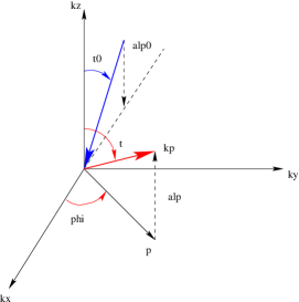
Figure 5: Wave vector decompositions. $\theta\in[0,\pi]$, and $\phi\in[0,2\pi]$.

We can introduce the normalized vector $\hat{\boldsymbol{k}}$ such that $\boldsymbol{k}=||\boldsymbol{k}||\,\hat{\boldsymbol{k}}$, and

$$\hat{\boldsymbol{k}}=\left(\begin{array}[]{c}\sin\phi\cos\theta\\ \sin\phi\sin\theta\\ \cos\phi\end{array}\right)\,,$$ (237)

In this way, for every function $F(\boldsymbol{k})$ which contains a Dirac distribution fixing the norm of the vector $\boldsymbol{k}$, we can define two new function $F(\hat{\boldsymbol{k}})$ and $F^{a}(\boldsymbol{p})$ (that we differentiate by their variable $\hat{\boldsymbol{k}}$ or $\boldsymbol{p}$) by

$$F(\boldsymbol{k})=\frac{(2\pi)^{3}}{K_{e}^{{}^{\prime}2}}\,\delta(||\boldsymbol{k}||-K_{e}^{\prime})\,F(\hat{\boldsymbol{k}})\,,$$ (238)

$$F(\boldsymbol{k})=\sum_{a=\pm}(2\pi)\delta(k_{z}-a\alpha^{\prime}_{e}(\boldsymbol{p}))\,F^{a}(\boldsymbol{p})\,,$$ (239)

such that

$$\int\frac{\rmd^{3}\boldsymbol{k}}{(2\pi)^{3}}\,\,F(\boldsymbol{k})=\int\rmd^{2}\hat{\boldsymbol{k}}\,\,F(\hat{\boldsymbol{k}})=\sum_{a=\pm}\int_{||\boldsymbol{p}||<K_{e}^{\prime}}\frac{\rmd^{2}\boldsymbol{p}}{(2\pi)^{2}}\,\,F^{a}(\boldsymbol{p})\,,$$ (240)

where $\rmd^{2}\hat{\boldsymbol{k}}=\sin\theta\rmd\theta\rmd\phi$ is the integration on the solid angle. We can connect the functions $F(\hat{\boldsymbol{k}})$ and $F(\boldsymbol{p})$ from equation (240) by

$$F^{a}(\hat{\boldsymbol{k}})\,\rmd^{2}\hat{\boldsymbol{k}}=F^{a}(\boldsymbol{p})\frac{\rmd^{2}\boldsymbol{p}}{(2\pi)^{2}}\,,$$ (241)

where we have defined for $a=\pm$

$$F^{a}(\hat{\boldsymbol{k}})=\Theta(ak_{z})\,F(\hat{\boldsymbol{k}})\,.$$ (242)

with $\Theta$ the Heaviside function. From Figure 5, we have

$$||\boldsymbol{p}||=K_{e}^{\prime}\sin\theta\,,$$ (243)

$$\alpha_{e}^{\prime}(\boldsymbol{p})=K_{e}^{\prime}|\cos\theta|\,,$$ (244)

since for a wave in the medium 1, we have $||\boldsymbol{k}||\simeq K_{e}^{\prime}$. Then

$$\frac{\rmd^{2}\boldsymbol{p}}{(2\pi)^{2}} =\frac{1}{(2\pi)^{2}}||\boldsymbol{p}||\rmd||\boldsymbol{p}||\rmd\phi\,,$$ (245)

$$=\frac{K_{e}^{\prime}\alpha^{\prime}_{e}(\boldsymbol{p})}{(2\pi)^{2}}\,\rmd\hat{\boldsymbol{k}}\,,$$ (246)

so that equation (241) can be transformed into

$$F^{a}(\hat{\boldsymbol{k}})=\frac{K_{e}^{\prime}\alpha_{e}^{\prime}(\boldsymbol{p})}{(2\pi)^{2}}\,F^{a}(\boldsymbol{p})\,.$$ (247)

In particular, for the Dirac distribution $F(\boldsymbol{k})=(2\pi)^{3}\,\delta(\boldsymbol{k}-\boldsymbol{k}_{0})$, we have

$$F(\hat{\boldsymbol{k}})=\delta(\hat{\boldsymbol{k}}-\hat{\boldsymbol{k}}_{0})\,,$$ (248)

$$F(\boldsymbol{p})=(2\pi)^{2}\,\delta(\boldsymbol{p}-\boldsymbol{p}_{0})\,,$$ (249)

and from equation (247)

$$\delta(\hat{\boldsymbol{k}}-\hat{\boldsymbol{k}}_{0})=K_{e}^{\prime}\alpha_{e}^{\prime}(\boldsymbol{p})\,\delta(\boldsymbol{p}-\boldsymbol{p}_{0})\,.$$ (250)

Hence, rather than using the variable $\boldsymbol{p}$ and $\boldsymbol{p}_{0}$ for $\overline{\boldsymbol{\mathcal{G}}}^{1a_{1}a_{0}}_{\ll SV\gg}$, we can introduce the vectors $\hat{\boldsymbol{k}}$ and $\hat{\boldsymbol{k}}_{0}$ and, defined similarly to equation (241), new tensors such that

$$\overline{\boldsymbol{\mathcal{G}}}^{1a1a_{0}}_{\ll SV\gg}(\boldsymbol{R},\hat{\boldsymbol{k}}|\boldsymbol{R}_{0},\hat{\boldsymbol{k}}_{0})=\frac{K_{e}^{\prime}\alpha^{\prime}_{e}(\boldsymbol{p})}{(2\pi)^{2}}\,\overline{\boldsymbol{\mathcal{G}}}^{1a1a_{0}}_{\ll SV\gg}(\boldsymbol{R},\boldsymbol{p}|\boldsymbol{R}_{0},\boldsymbol{p}_{0})\,\frac{K_{e}^{\prime}\alpha^{\prime}_{e}(\boldsymbol{p}_{0})}{(2\pi)^{2}}\,,$$ (251)

with $\boldsymbol{k}=K_{e}^{\prime}\hat{\boldsymbol{k}}=\boldsymbol{p}+a\alpha_{e}^{\prime}(\boldsymbol{p})\hat{\boldsymbol{e}}_{z}$ and $\boldsymbol{k}_{0}=K_{e}^{\prime}\hat{\boldsymbol{k}}_{0}=\boldsymbol{p}_{0}+a_{0}\alpha_{e}^{\prime}(\boldsymbol{p}_{0})\hat{\boldsymbol{e}}_{z}$. With this definition, the radiative transfer equation (236) is now

$$\hat{\boldsymbol{k}}\cdot\nabla\overline{\boldsymbol{\mathcal{G}}}^{1a1a_{0}}_{\ll SV\gg}(\boldsymbol{R},\hat{\boldsymbol{k}}|\boldsymbol{R}_{0},\hat{\boldsymbol{k}}_{0})+\kappa_{e}\,\overline{\boldsymbol{\mathcal{G}}}^{1a1a_{0}}_{\ll SV\gg}(\boldsymbol{R},\hat{\boldsymbol{k}}|\boldsymbol{R}_{0},\hat{\boldsymbol{k}}_{0})$$

$$=\frac{\delta(\hat{\boldsymbol{k}}-\hat{\boldsymbol{k}}_{0})}{(4\pi)^{2}}\,\delta_{a,a_{0}}\,\delta(\boldsymbol{R}-\boldsymbol{R}_{0})\,\overline{\boldsymbol{I}}_{\perp}^{1\,a}(\hat{\boldsymbol{k}})\otimes\overline{\boldsymbol{I}}_{\perp}^{1\,a}(\hat{\boldsymbol{k}})$$

$$+\sum_{a_{1}=\pm}\int_{a_{1}}\rmd^{2}\hat{\boldsymbol{k}}_{1}\,\overline{\boldsymbol{\mathcal{P}}}^{1a1a_{1}}(\hat{\boldsymbol{k}}|\hat{\boldsymbol{k}}_{1}):\overline{\boldsymbol{\mathcal{G}}}^{1a_{1}1a_{0}}_{\ll SV\gg}(\boldsymbol{R},\hat{\boldsymbol{k}}_{1}|\boldsymbol{R}_{0},\hat{\boldsymbol{k}}_{0})\,,$$ (252)

where $a=\mathrm{sgn}(\hat{\boldsymbol{k}}\cdot\hat{\boldsymbol{e}}_{z})$, $a_{0}=\mathrm{sgn}(\hat{\boldsymbol{k}}_{0}\cdot\hat{\boldsymbol{e}}_{z})$, and

$$\int_{a_{1}}\rmd^{2}\hat{\boldsymbol{k}}_{1}=\int_{a_{1}\hat{\boldsymbol{k}}_{z}\cdot\hat{\boldsymbol{e}}_{z}>0}\rmd^{2}\hat{\boldsymbol{k}}_{1}\,,$$ (253)

$$\overline{\boldsymbol{I}}_{\perp}^{1\,a}(\hat{\boldsymbol{k}})=\overline{\boldsymbol{I}}_{\perp}^{1\,a}(\boldsymbol{p})\,,$$ (254)

$$\overline{\boldsymbol{\mathcal{P}}}^{1a1a_{1}}(\hat{\boldsymbol{k}}|\hat{\boldsymbol{k}}_{1})=\frac{1}{(4\pi)^{2}}\,\overline{\boldsymbol{\mathcal{P}}}^{1a1a_{1}}(\boldsymbol{p}|\boldsymbol{p}_{1})\,.$$ (255)

The integration on $\hat{\boldsymbol{k}}_{1}$ is performed on the hemisphere defined by $a_{1}\hat{\boldsymbol{k}}_{1}\cdot\hat{\boldsymbol{e}}_{z}>0$ with $a_{1}=\pm$:

$$\left\{\begin{array}[]{cc}+\hat{\boldsymbol{k}}_{1}\cdot\hat{\boldsymbol{e}}_{z}>0&\Longleftrightarrow\theta_{1}\in[0,\pi/2]\,,\\ -\hat{\boldsymbol{k}}_{1}\cdot\hat{\boldsymbol{e}}_{z}>0&\Longleftrightarrow\theta_{1}\in[\pi/2,\pi]\,,\\ \end{array}\right.$$ (256)

with $\hat{\boldsymbol{k}}_{1}\cdot\hat{\boldsymbol{e}}_{z}=\cos\theta_{1}$. If we sum over all the propagation directions and define the tensor,

$$\overline{\boldsymbol{\mathcal{G}}}_{\ll SV\gg}(\boldsymbol{R},\hat{\boldsymbol{k}}|\boldsymbol{R}_{0},\hat{\boldsymbol{k}}_{0})=\sum_{a=\pm\,,a_{0}=\pm}\overline{\boldsymbol{\mathcal{G}}}^{1a1a_{0}}_{\ll SV\gg}(\boldsymbol{R},\hat{\boldsymbol{k}}|\boldsymbol{R}_{0},\hat{\boldsymbol{k}}_{0})$$ (257)

which does not distinguish if the wavevectors $\hat{\boldsymbol{k}}$ and $\hat{\boldsymbol{k}}_{0}$ are vertically directed upward or downward, the radiative transfer equation takes its classical form [5, 30, 57]:

$$\hat{\boldsymbol{k}}\cdot\nabla\overline{\boldsymbol{\mathcal{G}}}_{\ll SV\gg}(\boldsymbol{R},\hat{\boldsymbol{k}}|\boldsymbol{R}_{0},\hat{\boldsymbol{k}}_{0})+\kappa_{e}\overline{\boldsymbol{\mathcal{G}}}_{\ll SV\gg}(\boldsymbol{R},\hat{\boldsymbol{k}}|\boldsymbol{R}_{0},\hat{\boldsymbol{k}}_{0})$$

$$=\frac{\delta(\hat{\boldsymbol{k}}-\hat{\boldsymbol{k}}_{0})}{(4\pi)^{2}}\,\delta(\boldsymbol{R}-\boldsymbol{R}_{0})\overline{\boldsymbol{I}}_{\perp}(\hat{\boldsymbol{k}})\otimes\overline{\boldsymbol{I}}_{\perp}(\hat{\boldsymbol{k}})+\int\rmd^{2}\hat{\boldsymbol{k}}_{1}\,\overline{\boldsymbol{\mathcal{P}}}(\hat{\boldsymbol{k}}|\hat{\boldsymbol{k}}_{1}):\overline{\boldsymbol{\mathcal{G}}}_{\ll SV\gg}(\boldsymbol{R},\hat{\boldsymbol{k}}_{1}|\boldsymbol{R}_{0},\hat{\boldsymbol{k}}_{0})\,$$

(258)

with

$$\overline{\boldsymbol{I}}_{\perp}(\hat{\boldsymbol{k}}) =\overline{\boldsymbol{I}}-\hat{\boldsymbol{k}}\hat{\boldsymbol{k}}\,,$$ (259)

$$\overline{\boldsymbol{\mathcal{P}}}^{11}(\hat{\boldsymbol{k}}|\hat{\boldsymbol{k}}_{1}) =\sum_{a=\pm\,,a_{1}=\pm}\overline{\boldsymbol{\mathcal{P}}}^{1a1a_{1}}(\hat{\boldsymbol{k}}|\hat{\boldsymbol{k}}_{1})\,,$$ (260)

$$=\frac{1}{(4\pi)^{2}}\,n\,w(K_{e}^{\prime}\hat{\boldsymbol{k}}-K_{e}^{\prime}\hat{\boldsymbol{k}}_{1})\,\overline{\boldsymbol{C}}^{11}_{o}(K_{e}^{\prime}\hat{\boldsymbol{k}}|K_{e}^{\prime}\hat{\boldsymbol{k}}_{1})\otimes\overline{\boldsymbol{C}}^{11\,*}_{o}(K_{e}^{\prime}\hat{\boldsymbol{k}}|K_{e}^{\prime}\hat{\boldsymbol{k}}_{1})\,.$$ (261)

Thus, the tensor $\overline{\boldsymbol{\mathcal{G}}}_{\ll SV\gg}(\boldsymbol{R},\hat{\boldsymbol{k}}|\boldsymbol{R}_{0},\hat{\boldsymbol{k}}_{0})$ is the Green function of the radiative transfer equation where the source term is discrete, localized on $\boldsymbol{R}_{0}$, and emitting in the direction $\hat{\boldsymbol{k}}_{0}$ [5, 30, 57]. However, it is practically better to use the Green function $\overline{\boldsymbol{\mathcal{G}}}^{1a1a_{0}}_{\ll SV\gg}(\boldsymbol{R},\hat{\boldsymbol{k}}|\boldsymbol{R}_{0},\hat{\boldsymbol{k}}_{0})$ because we have to distinguish if the waves are upward or downward to write the boundary conditions. If we use the wave vectors $\hat{\boldsymbol{k}}$ and $\hat{\boldsymbol{k}}_{0}$ to write these boundary conditions, then

$$\overline{\boldsymbol{\mathcal{G}}}^{1-1a_{0}}_{\ll SV\gg}(Z=0,\hat{\boldsymbol{k}}|Z_{0},\hat{\boldsymbol{k}}_{0};\boldsymbol{P})$$ (262)

$$=\int_{\hat{\boldsymbol{k}}_{1}\cdot\hat{\boldsymbol{e}}_{z}>0}\rmd\hat{\boldsymbol{k}}_{1}\,\overline{\boldsymbol{\mathcal{R}}}^{01}_{\otimes\,<S>}(\hat{\boldsymbol{k}}|\hat{\boldsymbol{k}}_{1}):\overline{\boldsymbol{\mathcal{G}}}^{1+1a_{0}}_{\ll SV\gg}(Z=0,\hat{\boldsymbol{k}}_{1}|Z_{0},\hat{\boldsymbol{k}}_{0};\boldsymbol{P})\,,$$ (263)

$$\overline{\boldsymbol{\mathcal{G}}}^{1+1a_{0}}_{\ll SV\gg}(Z=-H,\hat{\boldsymbol{k}}|Z_{0},\hat{\boldsymbol{k}}_{0};\boldsymbol{P})$$ (264)

$$=\int_{\hat{\boldsymbol{k}}_{1}\cdot\hat{\boldsymbol{e}}_{z}<0}\rmd\hat{\boldsymbol{k}}_{1}\,\overline{\boldsymbol{\mathcal{R}}}^{21}_{\otimes\,<S>}(\hat{\boldsymbol{k}}|\hat{\boldsymbol{k}}_{1}):\overline{\boldsymbol{\mathcal{G}}}^{1-1a_{0}}_{\ll SV\gg}(Z=-H,\hat{\boldsymbol{k}}_{1}|Z_{0},\hat{\boldsymbol{k}}_{0};\boldsymbol{P})\,,$$ (265)

with

$$\overline{\boldsymbol{\mathcal{R}}}^{01}_{\otimes\,<S>}(\hat{\boldsymbol{k}}|\hat{\boldsymbol{k}}_{1})=\frac{K_{e}^{\prime}\alpha_{e}^{\prime}(\boldsymbol{p})}{(2\pi)^{2}}\,\overline{\boldsymbol{\mathcal{R}}}^{01}_{\otimes\,<S>}(\boldsymbol{p}|\boldsymbol{p}_{1};\boldsymbol{P}=\boldsymbol{0})\,,$$ (266)

$$\overline{\boldsymbol{\mathcal{R}}}^{21}_{\otimes\,<S>}(\hat{\boldsymbol{k}}|\hat{\boldsymbol{k}}_{1})=\frac{K_{e}^{\prime}\alpha_{e}^{\prime}(\boldsymbol{p})}{(2\pi)^{2}}\,\overline{\boldsymbol{\mathcal{R}}}^{21}_{\otimes\,<S>}(\boldsymbol{p}|\boldsymbol{p}_{1};\boldsymbol{P}=\boldsymbol{0})\,.$$ (267)

The relationship with the phenomenological radiative transfer theory is even clearer if we rewrite the radiative equation of section (11) in terms of $\hat{\boldsymbol{k}}$ by using the procedure that we have applied on $\overline{\boldsymbol{\mathcal{G}}}^{1a1a_{0}}_{\ll SV\gg}$:

$$\hat{\boldsymbol{k}}\cdot\nabla\overline{\boldsymbol{\mathcal{I}}}^{1a}_{\otimes\,d}(\boldsymbol{R},\hat{\boldsymbol{k}})+\kappa_{e}\,\overline{\boldsymbol{\mathcal{I}}}^{1a}_{\otimes\,d}(\boldsymbol{R},\hat{\boldsymbol{k}})=\sum_{a_{1}=\pm}\int\rmd^{2}\hat{\boldsymbol{k}}_{1}\,\overline{\boldsymbol{\mathcal{P}}}^{1a1a_{1}}(\hat{\boldsymbol{k}}|\hat{\boldsymbol{k}}_{1}):\overline{\boldsymbol{\mathcal{I}}}^{1a_{1}}_{\otimes\,d}(\boldsymbol{R},\hat{\boldsymbol{k}}_{1})+\boldsymbol{\mathcal{S}}^{1a}_{\otimes}(\boldsymbol{R},\hat{\boldsymbol{k}})\,,$$ (268)

where $\boldsymbol{\mathcal{S}}_{\otimes}^{1a}(\boldsymbol{R},\hat{\boldsymbol{k}})$ is the source term defined by:

$$\boldsymbol{\mathcal{S}}^{1a}_{\otimes}(\boldsymbol{R},\hat{\boldsymbol{k}})=\sum_{a_{1}=\pm}\int\rmd^{2}\hat{\boldsymbol{k}}_{1}\overline{\boldsymbol{\mathcal{P}}}^{1a1a_{1}}(\hat{\boldsymbol{k}}|\hat{\boldsymbol{k}}_{1}):\overline{\boldsymbol{\mathcal{I}}}^{1a_{1}}_{\otimes red}(\boldsymbol{R},\hat{\boldsymbol{k}}_{1})\,,$$ (269)

and $\overline{\boldsymbol{\mathcal{I}}}^{1a_{1}}_{\otimes\,red}(\boldsymbol{R},\hat{\boldsymbol{k}}_{1})$ the reduced intensity.

13 Muller matrix and tensorial product

Until now, to take into acount the polarization of the incident and scattered waves, we have used the tensorial product $\otimes$. However, in the optical and radar communities, it is customary to use Stokes vectors [16, 43]. In introducing the product $\odot$ between two vectors $\boldsymbol{E}^{1}$ and $\boldsymbol{E}^{2}$ by

$$\boldsymbol{E}^{1}\odot\boldsymbol{E}^{2}=\left(\begin{array}[]{c}E^{1}_{V}\,{E}^{2*}_{V}\\ {E}^{1}_{H}\,{E}^{2*}_{H}\\ {E}^{1}_{V}\,{E}^{2*}_{H}+{E}^{1}_{H}\,{E}^{2*}_{V}\\ \left({E}^{1}_{V}\,{E}^{2*}_{H}-{E}^{1}_{H}\,{E}^{2*}_{V}\right)/\rmi\end{array}\right)$$ (270)

for $\boldsymbol{E}^{1,2}=E^{1,2}_{V}\hat{\boldsymbol{e}}_{V}+E^{1,2}_{H}\hat{\boldsymbol{e}}_{H}$, the modified Stokes vectors of the incident and scattered waves are given by [6]

$$[\boldsymbol{I}^{0i}(\boldsymbol{p}_{0})]=e_{0}\,\boldsymbol{E}^{0i}(\boldsymbol{p}_{0})\odot\boldsymbol{E}^{0i}(\boldsymbol{p}_{0})=e_{0}\,\left(\begin{array}[]{c}|E^{0i}(\boldsymbol{p}_{0})_{V}|^{2}\\ |E^{0i}(\boldsymbol{p}_{0})_{H}|^{2}\\ 2\mathrm{Re}(E^{0i}(\boldsymbol{p}_{0})_{V}\,E^{0i}(\boldsymbol{p}_{0})_{H}^{*})\\ 2\mathrm{Im}(E^{0i}(\boldsymbol{p}_{0})_{V}\,E^{0i}(\boldsymbol{p}_{0})_{H}^{*})\end{array}\right)\,,$$ (275)

$$\left[\boldsymbol{I}^{0s}_{SV}(\boldsymbol{r})\right]=e_{0}\,\boldsymbol{E}^{0s}(\boldsymbol{r})\odot\boldsymbol{E}^{0s}(\boldsymbol{r})=e_{0}\,\left(\begin{array}[]{c}|E^{0s}_{SV}(\boldsymbol{r})_{V}|^{2}\\ |E^{0s}_{SV}(\boldsymbol{r})_{H}|^{2}\\ 2\mathrm{Re}(E^{0s}_{SV}(\boldsymbol{r})_{V}\,E^{0s}_{SV}(\boldsymbol{r})_{H}^{*})\\ 2\mathrm{Im}(E^{0s}_{SV}(\boldsymbol{r})_{V}\,E^{0s}_{SV}(\boldsymbol{r})_{H}^{*})\end{array}\right)\,.$$ (280)

To transform our previous equation using the tensorial product, in equations using the Stokes vector, we introduce the transformation $Tr^{\otimes\to\odot}$ by

$$Tr^{\otimes\to\odot}:\boldsymbol{\mathcal{I}}=\sum_{\beta,\beta^{\prime}=H,V}{\cal E}_{\beta\beta^{\prime}}\hat{\boldsymbol{e}}_{\beta}\otimes\hat{\boldsymbol{e}}^{*}_{\beta^{\prime}}\longrightarrow[I]=\left(\begin{array}[]{c}{\cal E}_{VV}\\ {\cal E}_{HH}\\ {\cal E}_{VH}+{\cal E}_{HV}\\ ({\cal E}_{VH}-{\cal E}_{HV})/\rmi\end{array}\right)\,.$$ (281)

With this transformation, we easily check the following property:

$$Tr^{\otimes\to\odot}\left(\boldsymbol{E}^{1}\otimes\boldsymbol{E}^{2\,*}\right)=\boldsymbol{E}^{1}\odot\boldsymbol{E}^{2}\,,$$ (282)

since for

$$\boldsymbol{E}^{1,2}=\sum_{\beta=H,V}E^{1,2}_{\beta}\,\hat{\boldsymbol{e}}_{\beta}\,,$$ (283)

we have

$$\boldsymbol{E}^{1}\otimes\boldsymbol{E}^{2\,*}=\sum_{\beta,\beta^{\prime}=H,V}E^{1}_{\beta}\,E^{2\,*}_{\beta^{\prime}}\hat{\boldsymbol{e}}_{\beta}\otimes\hat{\boldsymbol{e}}^{*}_{\beta^{\prime}}\,.$$ (284)

We can generalize the product $\odot$ and the transformation $\Tr^{\otimes\to\odot}$ to dyadics operators $\overline{\boldsymbol{f}}$ and $\overline{\boldsymbol{g}}$

$$\overline{\boldsymbol{f}}=\sum_{\beta,\beta^{\prime}=H,V}\,f_{\beta\beta^{\prime}}\hat{\boldsymbol{e}}_{\beta}\hat{\boldsymbol{e}}_{\beta^{\prime}}\,,\\ \overline{\boldsymbol{g}}=\sum_{\beta,\beta^{\prime}=H,V}\,g_{\beta\beta^{\prime}}\hat{\boldsymbol{e}}_{\beta}\hat{\boldsymbol{e}}_{\beta^{\prime}}\,,$$ (285)

acting on the vectors $\boldsymbol{E}^{1}$ and $\boldsymbol{E}^{2}$ defined by equation (283), in requiring the following properties:

$$\left(\overline{\boldsymbol{f}}\odot\overline{\boldsymbol{g}}\right)\cdot\left(\boldsymbol{E}^{1}\odot\boldsymbol{E}^{2}\right)=\left(\overline{\boldsymbol{f}}\cdot\boldsymbol{E}^{1}\right)\odot\left(\overline{\boldsymbol{g}}\cdot\boldsymbol{E}^{2}\right)\,,$$ (286)

$$\overline{\boldsymbol{f}}\odot\overline{\boldsymbol{g}}=Tr^{\otimes\to\odot}\left(\overline{\boldsymbol{f}}\otimes\overline{\boldsymbol{g}}^{*}\right)\,,$$ (287)

where the product $\cdot$ in the left hand side of equation (286) is the usual product between a vector and a matrix. Then, we obtain

$$\overline{\boldsymbol{f}}\odot\overline{\boldsymbol{g}}=\left(\begin{array}[]{llll}\scriptstyle\scriptstyle{f_{VV}g^{*}_{VV}}&\scriptstyle{f_{VH}g_{VH}^{*}}&\scriptstyle{\frac{1}{2}[f_{VV}g_{VH}^{*}+f_{VH}g_{VV}^{*}]}&\scriptstyle{\frac{\rmi}{2}[f_{VV}g_{VH}^{*}-f_{VH}g_{VV}^{*}]}\\ \scriptstyle{f_{HV}g^{*}_{HV}}&\scriptstyle{f_{HH}g_{HH}^{*}}&\scriptstyle{\frac{1}{2}[f_{HV}g_{HH}^{*}+f_{HH}g_{HV}^{*}]}&\scriptstyle{\frac{\rmi}{2}[f_{HV}g_{HH}^{*}-f_{HH}g_{HV}^{*}]}\\ \scriptstyle{\left[f_{VV}g^{*}_{HV}\right.}&\scriptstyle{\left[f_{VH}g^{*}_{HH}\right.}&\scriptstyle{\frac{1}{2}[f_{VV}g_{HH}^{*}+f_{HH}g_{VV}^{*}}&\scriptstyle{\frac{\rmi}{2}[f_{VV}g_{HH}^{*}-f_{HH}g_{VV}^{*}}\\ \scriptstyle{\quad\left.+f_{HV}g^{*}_{VV}\right]}&\scriptstyle{\quad\left.+f_{HH}g^{*}_{VH}\right]}&\scriptstyle{\quad+f_{VH}g_{HV}^{*}+f_{HV}g_{VH}^{*}]}&\scriptstyle{\quad-f_{VH}g_{HV}^{*}+f_{HV}g_{VH}^{*}]}\\ \scriptstyle{-\rmi[f_{VV}g^{*}_{HV}}&\scriptstyle{-\rmi[f_{VH}g^{*}_{HH}}&\scriptstyle{\frac{1}{2\rmi}[f_{VV}g_{HH}^{*}-f_{HH}g_{VV}^{*}}&\scriptstyle{\frac{1}{2}[f_{VV}g_{HH}^{*}+f_{HH}g_{VV}^{*}]}\\ \scriptstyle{\quad-f_{HV}g^{*}_{VV}]}&\scriptstyle{\quad-f_{HH}g^{*}_{VH}]}&\scriptstyle{\quad+f_{VH}g_{HV}^{*}-f_{HV}g_{VH}^{*}]}&\scriptstyle{\quad-f_{VH}g_{HV}^{*}-f_{HV}g_{VH}^{*}]}\end{array}\right),$$ (294)

(295)

and

$$Tr^{\otimes\to\odot}:\overline{\boldsymbol{\mathcal{M}}}=\sum_{\beta,\beta^{\prime},\beta_{0},\beta_{0}^{\prime}=H,V}\!\!\!\!\!\!\mathcal{M}_{\beta\beta^{\prime};\beta_{0}\beta_{0}^{\prime}}(\hat{\boldsymbol{e}}_{\beta}\otimes\hat{\boldsymbol{e}}_{\beta^{\prime}})(\hat{\boldsymbol{e}}_{\beta_{0}}\otimes\hat{\boldsymbol{e}}_{\beta_{0}^{\prime}})\longrightarrow[\overline{\boldsymbol{M}}]\,,$$

where

$$[\overline{\boldsymbol{M}}]=$$

$$\left(\begin{array}[]{cccc}\scriptstyle{\mathcal{M}_{VV;VV}}&\scriptstyle{\mathcal{M}_{VV;HH}}&\scriptstyle{\frac{1}{2}\left[\mathcal{M}_{VV;VH}+\mathcal{M}_{VV;HV}\right]}&\scriptstyle{\frac{\rmi}{2}\left[\mathcal{M}_{VV;VH}-\mathcal{M}_{VV;HV}\right]}\\ \scriptstyle{\mathcal{M}_{HH;VV}}&\scriptstyle{\mathcal{M}_{HH;HH}}&\scriptstyle{\frac{1}{2}\left[\mathcal{M}_{HH;VH}+\mathcal{M}_{HH;HV}\right]}&\scriptstyle{\frac{\rmi}{2}\left[\mathcal{M}_{HH;VH}-\mathcal{M}_{HH;HV}\right]}\\ \scriptstyle{\left[\mathcal{M}_{VH;VV}\right.}&\scriptstyle{\left[\mathcal{M}_{VH;HH}\right.}&\scriptstyle{\frac{1}{2}\left[\mathcal{M}_{VH;VH}+\mathcal{M}_{HV;HV}\right.}&\scriptstyle{\frac{\rmi}{2}\left[\mathcal{M}_{VH;VH}-\mathcal{M}_{HV;HV}\right.}\\ \scriptstyle{\quad\left.+\mathcal{M}_{HV;VV}\right]}&\scriptstyle{\quad\left.+\mathcal{M}_{HV;HH}\right]}&\scriptstyle{\quad\left.+\mathcal{M}_{VH;HV}+\mathcal{M}_{HV;VH}\right]}&\scriptstyle{\quad\left.-\mathcal{M}_{VH;HV}+\mathcal{M}_{HV;VH}\right]}\\ \scriptstyle{-\rmi\left[\mathcal{M}_{VH;VV}\right.}&\scriptstyle{-\rmi\left[\mathcal{M}_{VH;HH}\right.}&\scriptstyle{\frac{1}{2\rmi}\left[\mathcal{M}_{VH;VH}-\mathcal{M}_{HV;HV}\right.}&\scriptstyle{\frac{1}{2}\left[\mathcal{M}_{VH;VH}+\mathcal{M}_{HV;HV}\right.}\\ \scriptstyle{\quad\left.-\mathcal{M}_{HV;VV}\right]}&\scriptstyle{\quad\left.-\mathcal{M}_{HV;HH}\right]}&\scriptstyle{\quad\left.+\mathcal{M}_{VH;HV}-\mathcal{M}_{HV;VH}\right]}&\scriptstyle{\quad\left.-\mathcal{M}_{VH;HV}-\mathcal{M}_{HV;VH}\right]}\end{array}\right)\,.$$ (302)

As was demonstrated in section (2), the scattered field $\boldsymbol{E}^{0s}$ in the medium 0 is expressed as a function of the incident field $\boldsymbol{E}^{0i}$ with the help of the operators $\overline{\boldsymbol{f}}(\boldsymbol{p}|\boldsymbol{p}_{0})$:

$$\boldsymbol{E}^{0s}(\boldsymbol{r})=\frac{\rme^{\rmi K_{0}||\boldsymbol{r}||}}{||\boldsymbol{r}||}\overline{\boldsymbol{f}}(\boldsymbol{p}|\boldsymbol{p}_{0})\cdot\boldsymbol{E}^{0i}(\boldsymbol{p}_{0})\,.$$ (304)

The Stokes vector of the scattered wave can be related to the Stokes vector of the incident wave by the Muller matrix $[\overline{\boldsymbol{M}}]$:

$$[\boldsymbol{I}^{0s}_{SV}(\boldsymbol{r})]=\frac{1}{||\boldsymbol{r}||^{2}}[\overline{\boldsymbol{M}}(\boldsymbol{p}|\boldsymbol{p}_{0})]\cdot[\boldsymbol{I}^{0i}(\boldsymbol{p}_{0})]\,,$$ (305)

and from the properties in (286), we show that the Muller matrix is given by the product $\odot$ of the operators $\overline{\boldsymbol{f}}$ with itself:

$$[\overline{\boldsymbol{M}}(\boldsymbol{p}|\boldsymbol{p}_{0})] = \overline{\boldsymbol{f}}(\boldsymbol{p}|\boldsymbol{p}_{0})\odot\overline{\boldsymbol{f}}(\boldsymbol{p}|\boldsymbol{p}_{0})\,.$$ (306)

Furthermore, we have defined a tensorial cross-section which verifies

$$\overline{\boldsymbol{\sigma}}(\boldsymbol{p}_{0}|\boldsymbol{p}_{0})=\frac{4\pi}{A}\,\overline{\boldsymbol{f}}(\boldsymbol{p}|\boldsymbol{p}_{0})\otimes\overline{\boldsymbol{f}}(\boldsymbol{p}|\boldsymbol{p}_{0})\,.$$ (307)

With the transformation $Tr^{\otimes\to\odot}$, we can define a matrix cross-section $[\overline{\boldsymbol{\sigma}}(\boldsymbol{p}|\boldsymbol{p}_{0})]$ by

$$[\overline{\boldsymbol{\sigma}}(\boldsymbol{p}|\boldsymbol{p}_{0})]=Tr^{\otimes\to\odot}\left\{\overline{\boldsymbol{\sigma}}(\boldsymbol{p}|\boldsymbol{p}_{0})\right\}\,,$$ (308)

and from the properties in (287) and equations (306,307) we have:

$$[\overline{\boldsymbol{\sigma}}(\boldsymbol{p}|\boldsymbol{p}_{0})]=\frac{4\pi}{A}\,[\overline{\boldsymbol{M}}(\boldsymbol{p}|\boldsymbol{p}_{0})]\,.$$ (309)

Hence, the field scattered by the random medium is entirely characterized by its Muller matrix $[\overline{\boldsymbol{M}}(\boldsymbol{p}|\boldsymbol{p}_{0})]$, or equivalently by $[\sigma(\boldsymbol{p}|\boldsymbol{p}_{0})]$ which is the Muller matrix representation of the tensor $\sigma(\boldsymbol{p}|\boldsymbol{p}_{0})$. Moreover, we can rewrite all the equations previously obtained with the help of Muller matrices in transforming the product $\otimes$ by the product $\odot$ since we have

$$Tr^{\otimes\to\odot}\left(\overline{\boldsymbol{\mathcal{M}}}^{1}:\overline{\boldsymbol{\mathcal{M}}}^{2}\right)=\overline{\boldsymbol{M}}^{1}\cdot\overline{\boldsymbol{M}}^{2}\,$$ (310)

for

$$Tr^{\otimes\to\odot}\left(\overline{\boldsymbol{\mathcal{M}}}^{1,2}\right)=\overline{\boldsymbol{M}}^{1,2}\,.$$ (311)

The only non trivial transformation that we have to carry out is the right transpose of a tensor that we must replace by the right transpose of a Muller matrix and which is defined by

$$[Tr^{\otimes\to\odot}\left\{\overline{\boldsymbol{\mathcal{M}}}(\boldsymbol{p}|\boldsymbol{p}_{0})\right\}]^{T_{R}}=Tr^{\otimes\to\odot}\left\{[\overline{\boldsymbol{\mathcal{M}}}(\boldsymbol{p}|\boldsymbol{p}_{0})]^{T_{R}}\right\}\,.$$ (312)

The explicit expression of the right transpose of a Muller matrix is given in (E).

14 Recapitulation

In this section, we rewrite all the equations previously obtained in using the product $\odot$ and the simplifications described in section (12).

14.1 Scattering operators for the particles and the rough surfaces

For an incident wave inside medium 1:

$$\boldsymbol{E}^{1i}(\boldsymbol{r})=\boldsymbol{E}^{1i}(\hat{\boldsymbol{k}}_{0})\,\rme^{\rmi\,K_{e}\,\hat{\boldsymbol{k}}_{0}\cdot\boldsymbol{r}}\,,$$ (313)

the scattered field produced by a particle of permittivity $\tilde{\epsilon}_{s}=\epsilon_{s}-\epsilon_{1}+\epsilon_{e}$ surrounded by a medium of permittivity $\epsilon_{e}$ is described by a T matrix $\overline{\boldsymbol{t}}^{11}_{o}$:

$$\boldsymbol{E}^{1s}(\boldsymbol{r})=\int\rmd^{3}\boldsymbol{r}_{1}\,\rmd^{3}\boldsymbol{r}_{2}\,\,\overline{\boldsymbol{G}}^{\infty}_{1}(\boldsymbol{r},\boldsymbol{r}_{1})\cdot\overline{\boldsymbol{t}}^{11}_{o}(\boldsymbol{r}_{1},\boldsymbol{r}_{2})\cdot\boldsymbol{E}^{i}(\boldsymbol{r}_{2})\,,$$ (314)

where the Green function $\overline{\boldsymbol{G}}_{1}^{\,\infty}$ is

$$\overline{\boldsymbol{G}}_{1}^{\,\infty}(\boldsymbol{r}-\boldsymbol{r}_{0}) =\left(\overline{\boldsymbol{I}}+\frac{1}{K_{e}^{2}}\nabla\nabla\right)G_{1}^{\infty}(\boldsymbol{r}-\boldsymbol{r}_{0})\,,$$ (315)

$$G_{1}^{\infty}(\boldsymbol{r}-\boldsymbol{r}_{0}) =P.V.\frac{\rme^{\rmi\,K_{e}\,||\boldsymbol{r}-\boldsymbol{r}_{0}||}}{4\pi\,||\boldsymbol{r}-\boldsymbol{r}_{0}||}\,,$$ (316)

and $K^{2}_{e}=\epsilon_{e}\,K_{vac}^{2}$. In the far-field, the scattered field is a spherical wave:

$$\boldsymbol{E}^{1s}(\boldsymbol{r})=\frac{\rme^{\rmi K_{e}||\boldsymbol{r}||}}{||\boldsymbol{r}||}\,\overline{\boldsymbol{f}}(\hat{\boldsymbol{k}}|\hat{\boldsymbol{k}}_{0})\,,$$ (317)

and the operator $\overline{\boldsymbol{f}}(\hat{\boldsymbol{k}}|\hat{\boldsymbol{k}}_{0})$ has the following relationship with the T-matrix:

$$4\pi\,\overline{\boldsymbol{f}}(\hat{\boldsymbol{k}}|\hat{\boldsymbol{k}}_{0})=(\overline{\boldsymbol{I}}-\hat{\boldsymbol{k}}\hat{\boldsymbol{k}})\cdot\overline{\boldsymbol{t}}^{11}_{o}(K_{e}\hat{\boldsymbol{k}}|K_{e}\hat{\boldsymbol{k}}_{0})\cdot(\overline{\boldsymbol{I}}-\hat{\boldsymbol{k}}_{0}\hat{\boldsymbol{k}}_{0})\,.$$ (318)

For a spherical particle, an exact expression of $\overline{\boldsymbol{f}}(\hat{\boldsymbol{k}}|\hat{\boldsymbol{k}}_{0})$ is given by the Mie theory [67, 66].

14.2 Effective medium

The effective permittivity $\epsilon_{e}$ is solution of the following system of equations:

$$\epsilon_{e}\,K_{vac}^{2}\,\overline{\boldsymbol{I}}=\epsilon_{1}\,K_{vac}^{2}\,\overline{\boldsymbol{I}}+n\,\overline{\boldsymbol{C}}^{11}_{o}(\boldsymbol{k}_{0}|\boldsymbol{k}_{0})\,,$$ (319)

$$\overline{\boldsymbol{C}}^{11}_{o}(\boldsymbol{k}|\boldsymbol{k}_{0})=\overline{\boldsymbol{t}}^{11}_{o}(\boldsymbol{k}|\boldsymbol{k}_{0})+n\,\int\frac{\rmd^{3}\boldsymbol{k}_{1}}{(2\pi)^{3}}\,\,h(\boldsymbol{k}-\boldsymbol{k}_{1})\,\overline{\boldsymbol{t}}_{o}^{11}(\boldsymbol{k}|\boldsymbol{k}_{1})\cdot\overline{\boldsymbol{G}}_{1}^{\infty}(\boldsymbol{k}_{1})\cdot\overline{\boldsymbol{C}}^{11}_{o}(\boldsymbol{k}_{1}|\boldsymbol{k}_{0})\,,$$ (320)

where

$$h(\boldsymbol{k}-\boldsymbol{k}_{1})=\int\rmd^{3}\boldsymbol{r}_{\,}\,\exp(-\rmi\,(\boldsymbol{k}-\boldsymbol{k}_{1})\cdot\boldsymbol{r})\,[g(||\boldsymbol{r}||)-1]\,,$$ (321)

$$\overline{\boldsymbol{G}}_{1}^{\infty}(\boldsymbol{k})=\int\rmd^{3}\boldsymbol{r}\,\exp(-\rmi\boldsymbol{k}\cdot\boldsymbol{r})\,\overline{\boldsymbol{G}}_{1}^{\infty}(\boldsymbol{r})\,.$$ (322)

$\overline{\boldsymbol{C}}^{11}_{o}(\boldsymbol{k}|\boldsymbol{k}_{0})$ is the scattering operators of a particle located at the origin which takes into account the correlations with the other particles with the help of the pair distribution function $g(\boldsymbol{r})$.

14.3 Surface scattering operators

The fields scattered by the upper rough surface are described by the operators $\overline{\boldsymbol{R}}^{10}$, $\overline{\boldsymbol{T}}^{10}$, $\overline{\boldsymbol{R}}^{01}$, $\overline{\boldsymbol{T}}^{01}$, and the field scattered by the lower rough surface is described by the operator $\overline{\boldsymbol{R}}^{H\,21}$ such that
Incident field in the medium Scattered field in the medium $\overline{\boldsymbol{R}}^{10}$ 0 0 $\overline{\boldsymbol{T}}^{10}$ 0 1 $\overline{\boldsymbol{R}}^{01}$ 1 1 $\overline{\boldsymbol{T}}^{10}$ 1 0 $\overline{\boldsymbol{R}}^{H\,21}$ 1 1
For example, an upward incident plane wave in medium 1:

$$\boldsymbol{E}^{1i}(\boldsymbol{r})=\boldsymbol{E}^{1i}(\boldsymbol{p}_{0})\,\rme^{\rmi\,\boldsymbol{p}_{0}\cdot\boldsymbol{x}+\rmi\,\alpha_{e}(\boldsymbol{p}_{0})z}$$

is scattered into an upward wave in medium 0 and a downward wave in medium 1 and they are respectively given by

$$\boldsymbol{E}^{0s}(\boldsymbol{r})=\int\frac{\rmd^{2}\boldsymbol{p}}{(2\pi)^{2}}\,\,\rme^{\rmi\boldsymbol{p}\cdot\boldsymbol{x}+\rmi\,\alpha_{0}(\boldsymbol{p})z}\,\overline{\boldsymbol{T}}^{01}(\boldsymbol{p}|\boldsymbol{p}_{0})\cdot\boldsymbol{E}^{1i}(\boldsymbol{p}_{0})\,,$$ (323)

$$\boldsymbol{E}^{1s}(\boldsymbol{r})=\int\frac{\rmd^{2}\boldsymbol{p}}{(2\pi)^{2}}\,\,\rme^{\rmi\boldsymbol{p}\cdot\boldsymbol{x}-\rmi\,\alpha_{e}(\boldsymbol{p})z}\,\overline{\boldsymbol{R}}^{01}(\boldsymbol{p}|\boldsymbol{p}_{0})\cdot\boldsymbol{E}^{1i}(\boldsymbol{p}_{0})\,,$$ (324)

where $\alpha_{0}(\boldsymbol{p})=\sqrt{\epsilon_{0}K_{vac}^{2}-\boldsymbol{p}^{2}}$, and $\alpha_{e}(\boldsymbol{p})=\sqrt{\epsilon_{e}K_{vac}^{2}-\boldsymbol{p}^{2}}$. Since the mean plane of the lower rough surface is located at $z=-H$, the scattering operator $\overline{\boldsymbol{R}}^{H\,21}$ describing this surface is the scattering operator $\overline{\boldsymbol{R}}^{21}$ of a surface having its mean plane located at $z=0$ multiplied by a phase factor which depends on the thickness $H$:

$$\overline{\boldsymbol{R}}^{H\,21}(\boldsymbol{p}|\boldsymbol{p}_{0})=\rme^{\rmi(\alpha_{e}(\boldsymbol{p})+\alpha_{e}(\boldsymbol{p}_{0}))\cdot H}\,\overline{\boldsymbol{R}}^{21}(\boldsymbol{p}|\boldsymbol{p}_{0})\,.$$ (325)

With these scattering operators, we can construct the scattering operators $\overline{\boldsymbol{S}}$ of an homogeneous slab of permittivity $\epsilon_{e}$ having rough boundaries:

$$\begin{array}[]{ll}\overline{\boldsymbol{S}}^{\,1+\,1-}=\overline{\boldsymbol{R}}^{H\,21}+\overline{\boldsymbol{R}}^{H\,21}\cdot\overline{\boldsymbol{R}}^{01}\cdot\overline{\boldsymbol{R}}^{H\,21}+\dots\,,&\overline{\boldsymbol{S}}^{\,0+\,0-}=\overline{\boldsymbol{R}}^{10}+\overline{\boldsymbol{T}}^{01}\cdot\overline{\boldsymbol{S}}^{\,1+\,1-}\cdot\overline{\boldsymbol{T}}^{10}\,,\\ \overline{\boldsymbol{S}}^{\,1-\,1-}=\overline{\boldsymbol{R}}^{01}\cdot\overline{\boldsymbol{S}}^{\,1+\,1-}\,,&\overline{\boldsymbol{S}}^{\,1+\,0-}=\overline{\boldsymbol{S}}^{\,1+\,1-}\cdot\overline{\boldsymbol{T}}^{10}\,,\\ \overline{\boldsymbol{S}}^{\,1-\,1+}=\overline{\boldsymbol{R}}^{01}+\cdot\overline{\boldsymbol{R}}^{01}\cdot\overline{\boldsymbol{R}}^{H\,21}\cdot\overline{\boldsymbol{R}}^{01}+\dots\,,&\overline{\boldsymbol{S}}^{\,1-\,0-}=\overline{\boldsymbol{T}}^{10}+\overline{\boldsymbol{S}}^{\,1-\,1-}\cdot\overline{\boldsymbol{T}}^{10}\,,\\ \overline{\boldsymbol{S}}^{\,1+\,1+}=\overline{\boldsymbol{R}}^{H\,21}\cdot\overline{\boldsymbol{S}}^{\,1-\,1+}\,,&\overline{\boldsymbol{S}}^{\,0+\,1-}=\overline{\boldsymbol{T}}^{01}\cdot\overline{\boldsymbol{S}}^{\,1+\,1-}\,,\\ &\overline{\boldsymbol{S}}^{\,0+\,1+}=\overline{\boldsymbol{T}}^{01}+\overline{\boldsymbol{T}}^{01}\cdot\overline{\boldsymbol{S}}^{\,1+\,1+}\,.\end{array}$$ (326)

For example, $\overline{\boldsymbol{S}}^{\,1+\,0-}$ described the upward wave scattered inside the slab (medium 1) for an incident downward wave in medium 0.

14.4 Coherent field and coherent scattering cross-section

For an incident field $\boldsymbol{E}^{0i}(\boldsymbol{r})$ in medium 0

$$\boldsymbol{E}^{0i}(\boldsymbol{r})=\boldsymbol{E}^{0i}(\hat{\boldsymbol{k}}_{0})\,\rme^{\rmi\,K_{0}\,\hat{\boldsymbol{k}}_{0}\cdot\boldsymbol{r}}\,.$$ (327)

The average scattered field over the random medium is specular and is given by

$$\ll\boldsymbol{E}^{0s}(\boldsymbol{r})\gg_{SV}=\overline{\boldsymbol{S}}^{coh}(\boldsymbol{p}_{0})\cdot\boldsymbol{E}^{0i}(\hat{\boldsymbol{k}}_{0})\,\rme^{\rmi\,K_{0}\,\hat{\boldsymbol{k}}\cdot\boldsymbol{r}}\,,$$ (328)

with

$$\hbox to0.0pt{\hss${}K{}$}_{0}\hat{\boldsymbol{k}}_{0}=\boldsymbol{p}_{0}-\alpha_{0}(\boldsymbol{p}_{0})\hat{\boldsymbol{e}}_{z}\,,\qquad K_{0}\hat{\boldsymbol{k}}=\boldsymbol{p}_{0}+\alpha_{0}(\boldsymbol{p}_{0})\hat{\boldsymbol{e}}_{z}\,,$$ (329)

$$\hbox to0.0pt{\hss${}<{}$}\overline{\boldsymbol{S}}^{0+0-}(\boldsymbol{p}|\boldsymbol{p}_{0})>_{S}=(2\pi)^{2}\delta(\boldsymbol{p}-\boldsymbol{p}_{0})\,\overline{\boldsymbol{S}}^{coh}(\boldsymbol{p})\,.$$ (330)

Then, we found for the average cross-section

$$[\overline{\boldsymbol{\sigma}}^{coh}(\hat{\boldsymbol{k}}|\hat{\boldsymbol{k}}_{0})]=4\pi\,|\cos\theta_{0}|\,\delta(\hat{\boldsymbol{k}}-\hat{\boldsymbol{k}}_{0})\overline{\boldsymbol{S}}^{coh}(\boldsymbol{p}_{0})\odot\overline{\boldsymbol{S}}^{coh}(\boldsymbol{p}_{0})\,,$$ (331)

where $\boldsymbol{p}_{0}=K_{0}\,\hat{\boldsymbol{k}}_{0\,\perp}$ and $\cos\theta_{0}=\hat{\boldsymbol{k}}_{0}\cdot\hat{\boldsymbol{e}}_{z}$.

14.5 Incoherent cross-section

The incoherent Muller cross-section $[\overline{\boldsymbol{\sigma}}^{incoh}]$ is decomposed in four components:

$$[\overline{\boldsymbol{\sigma}}^{incoh}]=[\overline{\boldsymbol{\sigma}}^{incoh}_{L=0}]+[\overline{\boldsymbol{\sigma}}^{incoh}_{L=1}]+[\overline{\boldsymbol{\sigma}}_{Ladder}^{incoh}]+[\overline{\boldsymbol{\sigma}}_{Crossed}^{incoh}]\,.$$ (332)

14.6 Zero order scattering in volume

The first term $[\overline{\boldsymbol{\sigma}}^{incoh}_{L=0}]$ described only the incoherent scattering contribution due to the boundaries; the random medium is replaced by an homogeneous medium with the permittivity $\epsilon_{e}$:

$$[\overline{\boldsymbol{\sigma}}^{incoh}_{L=0}(\hat{\boldsymbol{k}}|\hat{\boldsymbol{k}}_{0})]=4\pi\cos\theta\,\overline{\boldsymbol{\mathcal{S}}}^{0+0-incoh}_{\odot<S>}(\hat{\boldsymbol{k}}|\hat{\boldsymbol{k}}_{0})\,,\\$$

where $\cos\theta=\hat{\boldsymbol{k}}\cdot\hat{\boldsymbol{e}}_{z}$ and $\overline{\boldsymbol{\mathcal{S}}}^{0+0-incoh}_{\odot<S>}$ is defined by

$$(2\pi)^{2}\delta(\boldsymbol{0})\,\overline{\boldsymbol{\mathcal{S}}}^{0+0-incoh}_{\odot<S>}(\hat{\boldsymbol{k}}|\hat{\boldsymbol{k}}_{0})=\frac{K_{0}^{2}\,\cos\theta}{(2\pi)^{2}}$$

$$\times\Big{\{}<\overline{\boldsymbol{S}}^{0+0-}(\boldsymbol{p}|\boldsymbol{p}_{0})\odot\overline{\boldsymbol{S}}^{0+0-}(\boldsymbol{p}|\boldsymbol{p}_{0})>_{S}-<\overline{\boldsymbol{S}}^{0+0-}(\boldsymbol{p}|\boldsymbol{p}_{0})>_{S}\odot<\overline{\boldsymbol{S}}^{0+0-}(\boldsymbol{p}|\boldsymbol{p}_{0})>_{S}\Big{\}}\,,$$

(333)

and $\boldsymbol{p}=K_{0}\,\hat{\boldsymbol{k}}_{\perp}$, $\boldsymbol{p}_{0}=K_{0}\,\hat{\boldsymbol{k}}_{0\perp}$.

14.7 First order scattering in volume

The second component $[\overline{\boldsymbol{\sigma}}^{incoh}_{L=1}]$ of the incoherent scattering cross-section contains only the single scattering contribution by the particles with the multiple scattering terms due to the boundaries:

$$[\overline{\boldsymbol{\sigma}}^{incoh}_{L=1}(\hat{\boldsymbol{k}}|\hat{\boldsymbol{k}}_{0})]=\sum_{a_{1},a_{2}=\pm}\int_{a_{1},a_{2}}\rmd^{2}\hat{\boldsymbol{k}}_{1}\,\rmd^{2}\hat{\boldsymbol{k}}_{2}\,\frac{\left(1-\rme^{-(a_{2}|\sec\theta_{2}|-a_{1}|\sec\theta_{1}|)\kappa_{e}\,H}\right)}{(a_{2}|\sec\theta_{2}|-a_{1}|\sec\theta_{1}|)\kappa_{e}}$$

$$\hbox to0.0pt{\hss${}\times{}$}\,\frac{4\pi\,\cos\theta}{|\cos\theta_{2}|}\,\overline{\boldsymbol{\mathcal{S}}}^{0+;1a_{2}}_{\odot\,<S>}(\hat{\boldsymbol{k}}|\hat{\boldsymbol{k}}_{2})\cdot\overline{\boldsymbol{\mathcal{P}}}_{\odot}^{1a_{2}1a_{1}}(\hat{\boldsymbol{k}}_{2}|\hat{\boldsymbol{k}}_{1})\cdot\overline{\boldsymbol{\mathcal{S}}}^{1a_{1};0-}_{\odot\,<S>}(\hat{\boldsymbol{k}}_{1}|\hat{\boldsymbol{k}}_{0})\,,$$ (334)

where $\sec\theta=1/\cos\theta$, and $\kappa_{e}=2\mathrm{Im}K_{e}$. The Muller matrix $\overline{\boldsymbol{\mathcal{P}}}_{\odot}^{1a_{2}1a_{1}}$ describing the scattering by one particle is defined by

$$\overline{\boldsymbol{\mathcal{P}}}_{\odot}^{1a_{2}1a_{1}}(\hat{\boldsymbol{k}}_{2}|\hat{\boldsymbol{k}}_{1})=\frac{1}{(4\pi)^{2}}n\,w(K_{e}^{\prime}\hat{\boldsymbol{k}}_{2}-K_{e}^{\prime}\hat{\boldsymbol{k}}_{1})\Theta(a_{2}\hat{\boldsymbol{k}}_{2z})\Theta(a_{1}\hat{\boldsymbol{k}}_{1z})$$

$$\hbox to0.0pt{\hss${}\qquad{}$}\qquad\times\overline{\boldsymbol{C}}^{11}_{o}(K_{e}^{\prime}\hat{\boldsymbol{k}}_{2}|K_{e}^{\prime}\hat{\boldsymbol{k}}_{1})\odot\overline{\boldsymbol{C}}^{11}_{o}(K_{e}^{\prime}\hat{\boldsymbol{k}}_{2}|K_{e}^{\prime}\hat{\boldsymbol{k}}_{1})\,,$$ (335)

where $\Theta$ is the Heaviside function, and $w$ is the structure factor of the random medium:

$$w(\boldsymbol{k}-\boldsymbol{k}_{0})=1+n\,\int\rmd^{3}\boldsymbol{r}\,\rme^{-\rmi(\boldsymbol{k}-\boldsymbol{k}_{0})\cdot\boldsymbol{r}}\,[g(\boldsymbol{r})-1]\,.$$ (336)

The Muller matrices describing the scattering at the boundaries are

$$(2\pi)^{2}\,\delta(\boldsymbol{0})\,\overline{\boldsymbol{\mathcal{S}}}_{\odot\,<S>}^{0+;1a_{2}}(\hat{\boldsymbol{k}}|\hat{\boldsymbol{k}}_{2})=\sqrt{\frac{\epsilon_{0}}{\epsilon^{\prime}_{e}}}\,\frac{K^{2}_{0}\cos\theta}{(2\pi)^{2}}\,<\overline{\boldsymbol{S}}^{0+1a_{2}}\left(\boldsymbol{p}|\boldsymbol{p}_{2}\right)\odot\overline{\boldsymbol{S}}^{0+1a_{2}}\left(\boldsymbol{p}|\boldsymbol{p}_{2}\right)>_{S}\,,$$ (337)

$$(2\pi)^{2}\,\delta(\boldsymbol{0})\,\overline{\boldsymbol{\mathcal{S}}}_{\odot\,<S>}^{1a_{1};0-}(\hat{\boldsymbol{k}}_{1}|\hat{\boldsymbol{k}}_{0})=\sqrt{\frac{\epsilon^{\prime}_{e}}{\epsilon_{0}}}\,\frac{K_{e}^{{}^{\prime}2}|\cos\theta_{1}|}{(2\pi)^{2}}\,<\overline{\boldsymbol{S}}^{1a_{1}\,0-}\left(\boldsymbol{p}_{1}|\boldsymbol{p}_{0}\right)\odot\overline{\boldsymbol{S}}^{1a_{1}\,0-}\left(\boldsymbol{p}_{1}|\boldsymbol{p}_{0}\right)>_{S}\,,$$

(338)

with

$$\begin{array}[]{ll}\boldsymbol{p}=K_{0}\hat{\boldsymbol{k}}_{\perp}\,,&\cos\theta=\hat{\boldsymbol{k}}\cdot\hat{\boldsymbol{e}}_{z}\\ \boldsymbol{p}_{2}=K_{e}^{\prime}\hat{\boldsymbol{k}}_{2\perp}\,,&\cos\theta_{2}=\hat{\boldsymbol{k}}_{2}\cdot\hat{\boldsymbol{e}}_{z}\\ \boldsymbol{p}_{1}=K_{e}^{\prime}\hat{\boldsymbol{k}}_{1\perp}\,,&\cos\theta_{1}=\hat{\boldsymbol{k}}_{1}\cdot\hat{\boldsymbol{e}}_{z}\\ \boldsymbol{p}_{0}=K_{0}\hat{\boldsymbol{k}}_{0\perp}\,,&\cos\theta_{0}=\hat{\boldsymbol{k}}_{0}\cdot\hat{\boldsymbol{e}}_{z}\end{array}\,.$$ (339)

In (F), we justify why in introducing the factors $\sqrt{\epsilon_{0}/\epsilon^{\prime}_{e}}$ and $\sqrt{\epsilon_{e}^{\prime}/\epsilon_{0}}$ in definitions (337) and (338), the operators $\overline{\boldsymbol{\mathcal{S}}}_{\odot\,<S>}^{0+;1a_{2}}$ and $\overline{\boldsymbol{\mathcal{S}}}_{\odot\,<S>}^{1a_{1};0-}$ match those used in the phenomenological radiative transfer theory. The integral in equations (171) is defined by

$$\int_{a_{1},a_{2}}\rmd^{2}\hat{\boldsymbol{k}}_{1}\,\rmd^{2}\hat{\boldsymbol{k}}_{2}=\int_{a_{1}\hat{\boldsymbol{k}}_{1}\cdot\hat{\boldsymbol{e}}_{z}>0}\rmd^{2}\hat{\boldsymbol{k}}_{1}\,\int_{a_{2}\hat{\boldsymbol{k}}_{2}\cdot\hat{\boldsymbol{e}}_{z}>0}\rmd^{2}\hat{\boldsymbol{k}}_{2}$$ (340)

where for $a_{1}=+$ the integration is on upper hemisphere, and for $a_{1}=-$ on the lower hemisphere:

$$\int_{a\hat{\boldsymbol{k}}\cdot\hat{\boldsymbol{e}}_{z}>0}\rmd^{2}\hat{\boldsymbol{k}}=\left\{\begin{array}[]{ll}\int_{0}^{\pi/2}\sin\theta\rmd\theta\int_{0}^{2\pi}\rmd\phi&\mbox{if }a=+\,,\\ \int_{\pi/2}^{\pi}\sin\theta\rmd\theta\int_{0}^{2\pi}\rmd\phi&\mbox{if }a=-\,,\end{array}\right.$$ (341)

14.8 Definition of the Green function $\overline{\boldsymbol{\mathcal{G}}}^{1a1a_{0}}_{\odot\ll SV\gg}$

To calculate the two other contributions $[\overline{\boldsymbol{\sigma}}^{incoh}_{Ladder}]$ and $[\overline{\boldsymbol{\sigma}}^{incoh}_{Crossed}]$, we need the Green function $\overline{\boldsymbol{\mathcal{G}}}^{11}_{\ll SV\gg}$ of the radiative transfer equation. This Green function is the Wigner transform of the Green function $\overline{\boldsymbol{G}}^{11}$ describing the propagation of the electric field in the medium I (See paper I):

$$\overline{\boldsymbol{\mathcal{G}}}^{11}_{\odot\ll SV\gg}(\boldsymbol{R},\boldsymbol{k}|\boldsymbol{R}_{0},\boldsymbol{k}_{0})=\int\rmd^{3}\boldsymbol{r}\,\rmd^{3}\boldsymbol{r}_{0}\,\,\rme^{-\rmi\boldsymbol{k}\cdot\boldsymbol{r}+\rmi\boldsymbol{k}_{0}\cdot\boldsymbol{r}_{0}}$$

$$\times\Big{[}\ll\overline{\boldsymbol{G}}^{11}_{SV}(\boldsymbol{R}+\frac{\boldsymbol{r}}{2},\boldsymbol{R}_{0}+\frac{\boldsymbol{r}_{0}}{2})\odot\overline{\boldsymbol{G}}^{11\,*}_{SV}(\boldsymbol{R}-\frac{\boldsymbol{r}}{2},\boldsymbol{R}_{0}-\frac{\boldsymbol{r}_{0}}{2})\gg_{SV}$$

$$-\ll\overline{\boldsymbol{G}}^{11}_{SV}(\boldsymbol{R}+\frac{\boldsymbol{r}}{2},\boldsymbol{R}_{0}+\frac{\boldsymbol{r}_{0}}{2})\gg_{SV}\odot\ll\overline{\boldsymbol{G}}^{11\,*}_{SV}(\boldsymbol{R}-\frac{\boldsymbol{r}}{2},\boldsymbol{R}_{0}-\frac{\boldsymbol{r}_{0}}{2})\gg_{SV}\Big{]}\,.$$ (342)

Under the quasi-uniform field approximation, we have [13]

$$\overline{\boldsymbol{\mathcal{G}}}^{11}_{\odot\ll SV\gg}(\boldsymbol{R},\boldsymbol{k}|\boldsymbol{R}_{0},\boldsymbol{k}_{0})=\frac{(2\pi)^{6}}{K_{e}^{{}^{\prime}4}}\,\delta(||\boldsymbol{k}||-K_{e}^{\prime})\delta(||\boldsymbol{k}_{0}||-K_{e}^{\prime})\,\overline{\boldsymbol{\mathcal{G}}}^{11}_{\odot\ll SV\gg}(\boldsymbol{R},\hat{\boldsymbol{k}}|\boldsymbol{R}_{0},\hat{\boldsymbol{k}}_{0})\,.$$ (343)

To write the boundary conditions, we have to distinguish between upward and downward waves, and we introduce

$$\overline{\boldsymbol{\mathcal{G}}}^{1a1a_{0}}_{\odot\ll SV\gg}(\boldsymbol{R},\hat{\boldsymbol{k}}|\boldsymbol{R}_{0},\hat{\boldsymbol{k}}_{0})=\Theta(a\hat{\boldsymbol{k}}\cdot\hat{\boldsymbol{e}}_{z})\Theta(a_{0}\hat{\boldsymbol{k}}_{0}\cdot\hat{\boldsymbol{e}}_{z})\,\overline{\boldsymbol{\mathcal{G}}}^{11}_{\odot\ll SV\gg}(\boldsymbol{R},\hat{\boldsymbol{k}}|\boldsymbol{R}_{0},\hat{\boldsymbol{k}}_{0})\,,$$ (344)

where $\Theta$ is the Heaviside function, and $a=\pm$, $a_{0}=\pm$. Finally, as the random medium and the rough surfaces are statistically homogeneous, we introduce the Fourier transform of the Green function along the horizontal coordinates $(X,Y)$:

$$\overline{\boldsymbol{\mathcal{G}}}^{1a1a_{0}}_{\odot\ll SV\gg}(Z,\hat{\boldsymbol{k}}|Z_{0},\hat{\boldsymbol{k}};\boldsymbol{P})=\int\rmd^{2}(\boldsymbol{X}-\boldsymbol{X}_{0})\,\rme^{-\rmi\boldsymbol{P}\cdot(\boldsymbol{X}-\boldsymbol{X}_{0})}\overline{\boldsymbol{\mathcal{G}}}^{1a1a_{0}}_{\odot\ll SV\gg}(\boldsymbol{R},\hat{\boldsymbol{k}}|\boldsymbol{R}_{0},\hat{\boldsymbol{k}}_{0})$$ (345)

with $\boldsymbol{R}=\boldsymbol{X}+Z\hat{\boldsymbol{e}}_{z}$ and $\boldsymbol{R}_{0}=\boldsymbol{X}_{0}+Z_{0}\hat{\boldsymbol{e}}_{z}$.

14.9 Radiative transfer equation

The matrices $\overline{\boldsymbol{\mathcal{G}}}^{1a1a_{0}}_{\odot\ll SV\gg}$ are the Green functions of the radiative transfer equation:

$$\hat{\boldsymbol{k}}\cdot\nabla_{\boldsymbol{P}}\,\overline{\boldsymbol{\mathcal{G}}}^{1a1a_{0}}_{\odot\ll SV\gg}(Z,\hat{\boldsymbol{k}}|Z_{0},\hat{\boldsymbol{k}}_{0};\boldsymbol{P})+\kappa_{e}\,\overline{\boldsymbol{\mathcal{G}}}^{1a_{1}1a_{0}}_{\odot\,\ll SV\gg}(Z,\hat{\boldsymbol{k}}|Z_{0},\hat{\boldsymbol{k}}_{0};\boldsymbol{P})$$

$$=\frac{\delta(\hat{\boldsymbol{k}}-\hat{\boldsymbol{k}}_{0})}{(4\pi)^{2}}\,\delta_{a,a_{0}}\,\delta(Z-Z_{0})\,\overline{\boldsymbol{I}}_{\perp}^{1\,a}(\hat{\boldsymbol{k}})\odot\overline{\boldsymbol{I}}_{\perp}^{1\,a}(\hat{\boldsymbol{k}})$$

$$+\sum_{a_{1}=\pm}\int_{a_{1}}\rmd^{2}\hat{\boldsymbol{k}}_{1}\,\overline{\boldsymbol{\mathcal{P}}}_{\odot}^{1a1a_{1}}(\hat{\boldsymbol{k}}|\hat{\boldsymbol{k}}_{1})\cdot\overline{\boldsymbol{\mathcal{G}}}^{1a_{1}1a_{0}}_{\odot\ll SV\gg}(Z,\hat{\boldsymbol{k}}_{1}|Z_{0},\hat{\boldsymbol{k}}_{0};\boldsymbol{P})\,,$$ (346)

where $a=\mathrm{sgn}(\hat{\boldsymbol{k}}\cdot\hat{\boldsymbol{e}}_{z})$, $a_{0}=\mathrm{sgn}(\hat{\boldsymbol{k}}_{0}\cdot\hat{\boldsymbol{e}}_{z})$, the differential operator $\nabla_{\boldsymbol{P}}$ is

$$\nabla_{\boldsymbol{P}}=\rmi\boldsymbol{P}+\hat{\boldsymbol{e}}_{z}\frac{\partial}{\partial Z}\,,$$ (347)

and the integral is defined by:

$$\int_{a_{1}}\rmd^{2}\hat{\boldsymbol{k}}_{1}=\int_{a_{1}\hat{\boldsymbol{k}}_{z}\cdot\hat{\boldsymbol{e}}_{z}>0}\rmd^{2}\hat{\boldsymbol{k}}_{1}\,.$$ (348)

The boundary conditions on the upper and lower surfaces are

$$\overline{\boldsymbol{\mathcal{G}}}^{1-1a_{0}}_{\odot\,\ll SV\gg}(Z=0,\hat{\boldsymbol{k}}|Z_{0},\hat{\boldsymbol{k}}_{0};\boldsymbol{P})$$

$$\qquad\qquad=\int_{\hat{\boldsymbol{k}}_{1}\cdot\hat{\boldsymbol{e}}_{z}>0}\rmd\hat{\boldsymbol{k}}_{1}\,\overline{\boldsymbol{\mathcal{R}}}^{01}_{\odot\,<S>}(\hat{\boldsymbol{k}}|\hat{\boldsymbol{k}}_{1})\cdot\overline{\boldsymbol{\mathcal{G}}}^{1+1a_{0}}_{\odot\ll SV\gg}(Z=0,\hat{\boldsymbol{k}}_{1}|Z_{0},\hat{\boldsymbol{k}}_{0};\boldsymbol{P})\,,$$ (349)

$$\overline{\boldsymbol{\mathcal{G}}}^{1+1a_{0}}_{\odot\ll SV\gg}(Z=-H,\hat{\boldsymbol{k}}|Z_{0},\hat{\boldsymbol{k}}_{0};\boldsymbol{P})$$

$$\qquad\qquad=\int_{\hat{\boldsymbol{k}}_{1}\cdot\hat{\boldsymbol{e}}_{z}<0}\rmd\hat{\boldsymbol{k}}_{1}\,\overline{\boldsymbol{\mathcal{R}}}^{21}_{\odot\,<S>}(\hat{\boldsymbol{k}}|\hat{\boldsymbol{k}}_{1})\cdot\overline{\boldsymbol{\mathcal{G}}}^{1-1a_{0}}_{\odot\ll SV\gg}(Z=-H,\hat{\boldsymbol{k}}_{1}|Z_{0},\hat{\boldsymbol{k}}_{0};\boldsymbol{P})\,,$$ (350)

with

$$(2\pi)^{2}\,\delta(\boldsymbol{0})\,\overline{\boldsymbol{\mathcal{R}}}^{01}_{\odot\,<S>}(\hat{\boldsymbol{k}}|\hat{\boldsymbol{k}}_{1}) =\frac{K_{e}^{{}^{\prime}2}|\cos\theta|}{(2\pi)^{2}}\,<\overline{\boldsymbol{R}}^{01}(\boldsymbol{p}|\boldsymbol{p}_{0})\odot\overline{\boldsymbol{R}}^{01\,*}(\boldsymbol{p}|\boldsymbol{p}_{0})>_{S}\,,$$ (351)

$$(2\pi)^{2}\,\delta(\boldsymbol{0})\,\overline{\boldsymbol{\mathcal{R}}}^{21}_{\odot\,<S>}(\hat{\boldsymbol{k}}|\hat{\boldsymbol{k}}_{1}) =\frac{K_{e}^{{}^{\prime}2}|\cos\theta|}{(2\pi)^{2}}\,<\overline{\boldsymbol{R}}^{21}(\boldsymbol{p}|\boldsymbol{p}_{0})\odot\overline{\boldsymbol{R}}^{21\,*}(\boldsymbol{p}|\boldsymbol{p}_{0})>_{S}\,,$$ (352)

and

$$\boldsymbol{p}=K_{e}^{\prime}\,\hat{\boldsymbol{k}}_{\perp}\,, \cos\theta=\hat{\boldsymbol{k}}\cdot\hat{\boldsymbol{e}}_{z}\,,$$ (353)

$$\boldsymbol{p}_{0}=K_{e}^{\prime}\,\hat{\boldsymbol{k}}_{0\perp}\,, \cos\theta_{0}=\hat{\boldsymbol{k}}_{0}\cdot\hat{\boldsymbol{e}}_{z}\,.$$ (354)

14.10 Integral equation

The integral form of the radiative transfer equation is

$$\overline{\boldsymbol{\mathcal{G}}}^{1a1a_{0}}_{\odot\,\ll SV\gg}(Z,\hat{\boldsymbol{k}}|Z_{0},\hat{\boldsymbol{k}}_{0};\boldsymbol{P})=\overline{\boldsymbol{\mathcal{G}}}^{1a1a_{0}}_{\odot\,\infty<S>}(Z,\hat{\boldsymbol{k}}|Z_{0},\hat{\boldsymbol{k}}_{0};\boldsymbol{P})+\sum_{a_{1}a_{2}}\,(4\pi)^{2}\int\rmd^{2}\hat{\boldsymbol{k}}_{1}\rmd^{2}\hat{\boldsymbol{k}}_{2}\,\rmd Z_{21}\,\,$$

$$\times\overline{\boldsymbol{\mathcal{G}}}^{1a1a_{2}}_{\odot\,\infty<S>}(Z,\hat{\boldsymbol{k}}|Z_{21},\hat{\boldsymbol{k}}_{2};\boldsymbol{P})\cdot\overline{\boldsymbol{\mathcal{P}}}^{1a_{2}1a_{1}}_{\odot}(\hat{\boldsymbol{k}}_{2}|\hat{\boldsymbol{k}}_{1})\cdot\overline{\boldsymbol{\mathcal{G}}}^{1a_{1}a_{0}}_{\odot\,\ll SV\gg}(Z_{21},\hat{\boldsymbol{k}}_{1}|Z_{0},\hat{\boldsymbol{k}}_{0};\boldsymbol{P})\,,$$ (355)

where

$$\overline{\boldsymbol{\mathcal{G}}}^{1a1a_{0}}_{\odot\,\infty<S>}(Z,\hat{\boldsymbol{k}}|Z_{0},\hat{\boldsymbol{k}}_{0};\boldsymbol{P})=\overline{\boldsymbol{\mathcal{G}}}^{1a1a_{0}}_{\odot\,\infty}(Z,\hat{\boldsymbol{k}}|Z_{0},\hat{\boldsymbol{k}}_{0};\boldsymbol{P})+\overline{\boldsymbol{\mathcal{G}}}^{1a1a_{0}}_{\odot\,<S>}(Z,\hat{\boldsymbol{k}}|Z_{0},\hat{\boldsymbol{k}}_{0};\boldsymbol{P})\,,$$ (356)

and

$$\overline{\boldsymbol{\mathcal{G}}}^{1a1a_{0}}_{\odot\,\infty}(Z,\hat{\boldsymbol{k}}|Z_{0},\hat{\boldsymbol{k}}_{0};\boldsymbol{P})=\frac{\delta(\hat{\boldsymbol{k}}-\hat{\boldsymbol{k}}_{0})}{(4\pi)^{2}\,|\cos\theta|}\overline{\boldsymbol{I}}^{1a}_{\perp}(\hat{\boldsymbol{k}})\odot\overline{\boldsymbol{I}}^{1a}_{\perp}(\hat{\boldsymbol{k}})\,\delta_{a,a_{0}}\,\delta_{a,sgn(Z-Z_{0})}\$$

$$\hbox to0.0pt{\hss${}\times{}$}\exp\left(-a(\kappa_{e}+\rmi\hat{\boldsymbol{k}}\cdot\boldsymbol{P})(Z-Z_{0})/|\cos\theta|\right)\,,$$ (357)

$$\overline{\boldsymbol{\mathcal{G}}}^{1a1a_{0}}_{\odot\,<S>}(Z,\hat{\boldsymbol{k}}|Z_{0},\hat{\boldsymbol{k}}_{0};\boldsymbol{P})=\frac{1}{(4\pi)^{2}\,|\cos\theta_{0}|}\,\overline{\boldsymbol{\mathcal{S}}}^{1a1a_{0}}_{\odot\,<S>}(\hat{\boldsymbol{k}}|\hat{\boldsymbol{k}}_{0})$$

$$\hbox to0.0pt{\hss${}\times{}$}\exp\left(-a(\kappa_{e}+\rmi\hat{\boldsymbol{k}}\cdot\boldsymbol{P})Z/|\cos\theta|+a_{0}(\kappa_{e}+\rmi\hat{\boldsymbol{k}}_{0}\cdot\boldsymbol{P})Z_{0}/|\cos\theta_{0}|\right)\,,$$ (358)

and

$$(2\pi)^{2}\,\delta(\boldsymbol{0})\,\overline{\boldsymbol{\mathcal{S}}}^{1a1a_{0}}_{\odot\,<S>}(\hat{\boldsymbol{k}}|\hat{\boldsymbol{k}}_{0})=\frac{K_{e}^{{}^{\prime}2}|\cos\theta|}{(2\pi)^{2}}\,<\overline{\boldsymbol{S}}^{1a1a_{0}}(\boldsymbol{p}|\boldsymbol{p}_{0})\odot\overline{\boldsymbol{S}}^{1a1a_{0}\,*}(\boldsymbol{p}|\boldsymbol{p}_{0})>_{S}\,,$$ (359)

with

$$\boldsymbol{p}=K_{e}^{\prime}\,\hat{\boldsymbol{k}}_{\perp}\,, \cos\theta=\hat{\boldsymbol{k}}\cdot\hat{\boldsymbol{e}}_{z}\,,$$ (360)

$$\boldsymbol{p}_{0}=K_{e}^{\prime}\,\hat{\boldsymbol{k}}_{0\perp}\,, \cos\theta_{0}=\hat{\boldsymbol{k}}_{0}\cdot\hat{\boldsymbol{e}}_{z}\,.$$ (361)

14.11 Ladder terms

The third contribution to the incoherent scattering cross-section, which contains second order and higher scattering contributions by the particles, is

$$[\overline{\boldsymbol{\sigma}}^{incoh}_{Ladder}(\hat{\boldsymbol{k}}|\hat{\boldsymbol{k}}_{0})]=\sum_{a_{1},a_{2},a_{3},a_{4}=\pm}\int_{-H}^{0}\rmd Z_{43}\rmd Z_{21}\int_{a_{1},a_{2},a_{3},a_{4}}\!\!\!\!\!\!\!\!\!\!\!\rmd^{2}\hat{\boldsymbol{k}}_{1}\,\rmd^{2}\hat{\boldsymbol{k}}_{2}\,\rmd^{2}\hat{\boldsymbol{k}}_{3}\,\rmd^{2}\hat{\boldsymbol{k}}_{4}\,$$

$$\times\frac{(4\pi)^{3}\,\cos\theta}{|\cos\theta_{4}|}\,\exp\left(a_{4}\,\kappa_{e}Z_{43}|\sec\theta_{4}|-a_{1}\,\kappa_{e}Z_{21}|\sec\theta_{1}|\right)\,\overline{\boldsymbol{\mathcal{S}}}^{0+;1a_{4}}_{\odot\,<S>}(\hat{\boldsymbol{k}}|\hat{\boldsymbol{k}}_{4})$$

$$\cdot\overline{\boldsymbol{\mathcal{P}}}_{\odot}^{1a_{4}1a_{3}}(\hat{\boldsymbol{k}}_{4}|\hat{\boldsymbol{k}}_{3})\cdot\overline{\boldsymbol{\mathcal{G}}}^{1a_{3}1a_{2}}_{\odot\,\ll SV\gg}(Z_{43},\hat{\boldsymbol{k}}_{3}|Z_{21},\hat{\boldsymbol{k}}_{2};\boldsymbol{P}=\boldsymbol{0})\cdot\overline{\boldsymbol{\mathcal{P}}}_{\odot}^{1a_{2}1a_{1}}(\hat{\boldsymbol{k}}_{2}|\hat{\boldsymbol{k}}_{1})\cdot\overline{\boldsymbol{\mathcal{S}}}^{1a_{1};0-}_{\odot\,<S>}(\hat{\boldsymbol{k}}_{1}|\hat{\boldsymbol{k}}_{0})\,,$$

(362)

with $\cos\theta=\hat{\boldsymbol{k}}\cdot\hat{\boldsymbol{e}}_{z}$, $\cos\theta_{1}=\hat{\boldsymbol{k}}_{1}\cdot\hat{\boldsymbol{e}}_{z}$, $\cos\theta_{4}=\hat{\boldsymbol{k}}_{4}\cdot\hat{\boldsymbol{e}}_{z}$ and

$$\int_{a_{1},a_{2},a_{3},a_{4}}\!\!\!\!\!\!\!\!\!\!\!\!\rmd^{2}\hat{\boldsymbol{k}}_{1}\,\rmd^{2}\hat{\boldsymbol{k}}_{2}\,\rmd^{2}\hat{\boldsymbol{k}}_{3}\,\rmd^{2}\hat{\boldsymbol{k}}_{4}=\int_{a_{1}\hat{\boldsymbol{k}}_{z}\cdot\hat{\boldsymbol{e}}_{z}>0}\!\!\!\!\!\!\!\!\!\!\rmd^{2}\hat{\boldsymbol{k}}_{1}\int_{a_{2}\hat{\boldsymbol{k}}_{z}\cdot\hat{\boldsymbol{e}}_{z}>0}\!\!\!\!\!\!\!\!\!\!\rmd^{2}\hat{\boldsymbol{k}}_{2}\int_{a_{3}\hat{\boldsymbol{k}}_{z}\cdot\hat{\boldsymbol{e}}_{z}>0}\!\!\!\!\!\!\!\!\!\!\rmd^{2}\hat{\boldsymbol{k}}_{3}\int_{a_{4}\hat{\boldsymbol{k}}_{z}\cdot\hat{\boldsymbol{e}}_{z}>0}\!\!\!\!\!\!\!\!\!\!\rmd^{2}\hat{\boldsymbol{k}}_{4}\,.$$ (363)

14.12 Most-crossed contributions

The fourth contribution of the incoherent scattering cross-section, which describes the enhanced backscattering phenomenon, is

$$[\overline{\boldsymbol{\sigma}}^{incoh}_{Crossed}(\hat{\boldsymbol{k}}|\hat{\boldsymbol{k}}_{0})]=\sum_{a_{1},a_{2},a_{3},a_{4}=\pm}\int_{-H}^{0}\rmd Z_{43}\rmd Z_{21}\int_{a_{1},a_{2},a_{3},a_{4}}\!\!\!\!\!\!\!\!\!\!\!\rmd^{2}\hat{\boldsymbol{k}}_{1}\,\rmd^{2}\hat{\boldsymbol{k}}_{2}\,\rmd^{2}\hat{\boldsymbol{k}}_{3}\,\rmd^{2}\hat{\boldsymbol{k}}_{4}\,$$

$$\times\frac{(4\pi)^{3}\,|\cos\theta_{0}|}{|\cos\theta^{-}_{4}|}\,\exp\left(\rmi\,a_{4}Z_{43}K_{e}^{\prime}(|\cos\theta_{4}^{+}|-|\cos\theta_{4}^{-}|)-\rmi\,a_{1}Z_{21}K_{e}^{\prime}(|\cos\theta_{1}^{+}|-|\cos\theta_{1}^{-}|)\right)\,$$

$$\times\exp\Big{(}a_{4}\,\kappa_{e}Z_{43}(|\sec\theta_{4}^{+}|+|\sec\theta_{4}^{-}|)/2-a_{1}\,\kappa_{e}Z_{21}(|\sec\theta_{1}^{+}|+|\sec\theta_{1}^{-}|)/2\Big{)}$$

$$\times\Big{[}\overline{\boldsymbol{\mathcal{S}}}^{0+;1a_{4}}_{\odot\,<S>}(-\hat{\boldsymbol{k}}_{0}|\hat{\boldsymbol{k}}_{4})\cdot\overline{\boldsymbol{\mathcal{P}}}_{\odot}^{1a_{4}1a_{3}}(\hat{\boldsymbol{k}}_{4}|\hat{\boldsymbol{k}}_{3})\cdot\overline{\boldsymbol{\mathcal{G}}}^{1a_{3}1a_{2}}_{\odot\ll SV\gg}(Z_{43},\hat{\boldsymbol{k}}_{3}|Z_{21},\hat{\boldsymbol{k}}_{2};\boldsymbol{P})$$

$$\cdot\overline{\boldsymbol{\mathcal{P}}}_{\odot}^{1a_{2}1a_{1}}(\hat{\boldsymbol{k}}_{2}|\hat{\boldsymbol{k}}_{1})\cdot\overline{\boldsymbol{\mathcal{S}}}^{1a_{1};0-}_{\odot\,<S>}(\hat{\boldsymbol{k}}_{1}|\hat{\boldsymbol{k}}_{0})\Big{]}^{T_{R}}\,,$$ (364)

where the right transposed ${}^{T_{R}}$ of a Muller matrix is defined in E and

$$\boldsymbol{P}=K_{0}(\hat{\boldsymbol{k}}_{\perp}+\hat{\boldsymbol{k}}_{0\perp})\,,\qquad\cos\theta_{0}=\hat{\boldsymbol{k}}_{0}\cdot\hat{\boldsymbol{e}}_{z}\,.$$ (365)

The definition of the angles $\theta_{4}^{\pm}$ and $\theta_{1}^{\pm}$ depends on the matrix $\overline{\boldsymbol{\mathcal{S}}}^{0+;1a_{4}}_{\odot\,<S>}$ and $\overline{\boldsymbol{\mathcal{S}}}^{1a_{1};0-}_{\odot\,<S>}$. Each of these matrices has a coherent and an incoherent part:

$$\overline{\boldsymbol{\mathcal{S}}}^{0+;1a_{0}}_{\odot\,<S>}(\hat{\boldsymbol{k}}|\hat{\boldsymbol{k}}_{0})=\overline{\boldsymbol{\mathcal{S}}}^{0+;1a_{0}\,incoh}_{\odot\,<S>}(\hat{\boldsymbol{k}}|\hat{\boldsymbol{k}}_{0})+\delta(\hat{\boldsymbol{k}}^{t}-\hat{\boldsymbol{k}}_{0})\overline{\boldsymbol{\mathcal{S}}}^{0+;1a_{0}\,coh}_{\odot\,<S>}(\hat{\boldsymbol{k}}_{0})\,,$$ (366)

$$\overline{\boldsymbol{\mathcal{S}}}^{1a;0-}_{\odot\,<S>}(\hat{\boldsymbol{k}}|\hat{\boldsymbol{k}}_{0})=\overline{\boldsymbol{\mathcal{S}}}^{1a;0-\,incoh}_{\odot\,<S>}(\hat{\boldsymbol{k}}|\hat{\boldsymbol{k}}_{0})+\delta(\hat{\boldsymbol{k}}^{t}-\hat{\boldsymbol{k}}_{0})\,\overline{\boldsymbol{\mathcal{S}}}^{1a;0-\,coh}_{\odot\,<S>}(\hat{\boldsymbol{k}}_{0})\,,$$ (367)

where $\hat{\boldsymbol{k}}^{t}$ and $\hat{\boldsymbol{k}}_{0}$ are related by the Fresnel law:

$$K_{0}\,\hat{\boldsymbol{k}}^{t}_{\perp}=K_{e}^{\prime}\hat{\boldsymbol{k}}_{0\,\perp}\,\mbox{for}\quad\overline{\boldsymbol{\mathcal{S}}}^{0+;1a_{4}}_{\odot\,<S>}(\hat{\boldsymbol{k}}|\hat{\boldsymbol{k}}_{0})\,,$$ (368)

$$K_{e}^{\prime}\,\hat{\boldsymbol{k}}^{t}_{\perp}=K_{0}\,\hat{\boldsymbol{k}}_{0\perp}\,\mbox{for}\quad\overline{\boldsymbol{\mathcal{S}}}^{1a;0-}_{\odot\,<S>}(\hat{\boldsymbol{k}}|\hat{\boldsymbol{k}}_{0})\,.$$ (369)

For the incoherent part, the angles are defined by

$$|\cos\theta_{4}^{+}|=\sqrt{1-(\hat{\boldsymbol{k}}_{4\perp}+\boldsymbol{P}/2K_{e}^{\prime})^{2}}\,,$$ (370)

$$|\cos\theta_{4}^{-}|=\sqrt{1-(\hat{\boldsymbol{k}}_{4\perp}-\boldsymbol{P}/2K_{e}^{\prime})^{2}}\,,$$ (371)

$$|\cos\theta_{1}^{+}|=\sqrt{1-(\hat{\boldsymbol{k}}_{1\perp}+\boldsymbol{P}/2K_{e}^{\prime})^{2}}\,,$$ (372)

$$|\cos\theta_{1}^{-}|=\sqrt{1-(\hat{\boldsymbol{k}}_{1\perp}-\boldsymbol{P}/2K_{e}^{\prime})^{2}}\,,$$ (373)

and for the coherent part we have:

$$|\cos\theta_{4}^{+}|=\sqrt{1-(K_{0}\hat{\boldsymbol{k}}_{\perp}/K_{e}^{\prime})^{2}}\,,$$ (374)

$$|\cos\theta_{4}^{-}|=\sqrt{1-(K_{0}\hat{\boldsymbol{k}}_{0\perp}/K_{e}^{\prime})^{2}}\,,$$ (375)

$$|\cos\theta_{1}^{+}|=|\cos\theta_{4}^{-}|\,,$$ (376)

$$|\cos\theta_{1}^{-}|=|\cos\theta_{4}^{+}|\,.$$ (377)

We notice that in the backscattering direction, we have $\hat{\boldsymbol{k}}=-\hat{\boldsymbol{k}}_{0}$ and then $\boldsymbol{P}=\boldsymbol{0}$, $\cos\theta_{4}^{+}=\cos\theta_{4}^{-}$, $\cos\theta_{1}^{+}=\cos\theta_{1}^{-}$. In this direction, the crossed contribution differs from the ladder approximation only by the presence of the right transpose ${}^{T_{R}}$ around the Muller matrix in the equation (364).

14.13 Other Formulation

We can also calculate the incoherent cross-section in introducing the specific diffusive specific intensity $\overline{\boldsymbol{\mathcal{I}}}^{1a}_{\odot\,d}(Z,\hat{\boldsymbol{k}};\boldsymbol{P})$ which verifies the usual phenomenological radiative transfer equation:

$$\hat{\boldsymbol{k}}\cdot\nabla_{\boldsymbol{P}}\,\overline{\boldsymbol{\mathcal{I}}}^{1a}_{\odot\,d}(Z,\hat{\boldsymbol{k}};\boldsymbol{P})+\kappa_{e}\,\overline{\boldsymbol{\mathcal{I}}}^{1a}_{\odot\,d}(Z,\hat{\boldsymbol{k}};\boldsymbol{P})=\sum_{a_{1}=\pm}\int\rmd^{2}\hat{\boldsymbol{k}}_{1}\,\overline{\boldsymbol{\mathcal{P}}}_{\odot}^{1a1a_{1}}(\hat{\boldsymbol{k}}|\hat{\boldsymbol{k}}_{1})\cdot\overline{\boldsymbol{\mathcal{I}}}^{1a_{1}}_{\odot\,d}(Z,\hat{\boldsymbol{k}}_{1};\boldsymbol{P})$$

$$\hbox to0.0pt{\hss${}+{}$}\boldsymbol{\mathcal{S}}^{1a}_{\odot}(Z,\hat{\boldsymbol{k}};\boldsymbol{P})\,,$$ (378)

where $\boldsymbol{S}^{1a}_{\odot}(Z,\hat{\boldsymbol{k}};\boldsymbol{P})$ is the source term defined by:

$$\boldsymbol{\mathcal{S}}^{1a}_{\odot}(Z,\hat{\boldsymbol{k}};\boldsymbol{P})=\sum_{a_{1}=\pm}\int\rmd^{2}\hat{\boldsymbol{k}}_{1}\overline{\boldsymbol{\mathcal{P}}}_{\odot}^{1a1a_{1}}(\hat{\boldsymbol{k}}|\hat{\boldsymbol{k}}_{1})\cdot\overline{\boldsymbol{\mathcal{I}}}^{1a_{1}}_{\odot red}(Z,\hat{\boldsymbol{k}}_{1};\boldsymbol{P})\,,$$ (379)

and $\overline{\boldsymbol{\mathcal{I}}}^{1a_{1}}_{\odot red}(Z,\hat{\boldsymbol{k}}_{1};\boldsymbol{P})$ the reduced specific intensity [6]:

$$\overline{\boldsymbol{\mathcal{I}}}_{\odot\,red}^{1a_{1}}(Z_{1},\hat{\boldsymbol{k}}_{1};\boldsymbol{P})=\overline{\boldsymbol{\mathcal{S}}}^{1a_{1}0-}_{\odot\,<S>}(\hat{\boldsymbol{k}}_{1}|\hat{\boldsymbol{k}}_{0})\,\exp\left(-a_{1}\,(\kappa_{e}+\rmi\,\hat{\boldsymbol{k}}\cdot\boldsymbol{P})Z_{1}/|\cos\theta_{1}|\right)\,,$$ (380)

with $\cos\theta_{1}=\hat{\boldsymbol{k}}_{z}\cdot\hat{\boldsymbol{e}}_{z}$. The boundary conditions necessary to solve the radiative transfer equation are

$$\overline{\boldsymbol{\mathcal{I}}}^{1-}_{\odot\,d}(Z=0,\hat{\boldsymbol{k}};\boldsymbol{P})=\int_{\hat{\boldsymbol{k}}_{1}\cdot\hat{\boldsymbol{e}}_{z}>0}\rmd\hat{\boldsymbol{k}}_{1}\,\overline{\boldsymbol{\mathcal{R}}}^{01}_{\odot\,<S>}(\hat{\boldsymbol{k}}|\hat{\boldsymbol{k}}_{1})\cdot\overline{\boldsymbol{\mathcal{I}}}^{1+}_{\odot\,d}(Z=0,\hat{\boldsymbol{k}}_{1};\boldsymbol{P})\,,$$ (381)

$$\overline{\boldsymbol{\mathcal{I}}}^{1+}_{\odot\,d}(Z=-H,\hat{\boldsymbol{k}};\boldsymbol{P})=\int_{\hat{\boldsymbol{k}}_{1}\cdot\hat{\boldsymbol{e}}_{z}<0}\rmd\hat{\boldsymbol{k}}_{1}\,\overline{\boldsymbol{\mathcal{R}}}^{21}_{\odot\,<S>}(\hat{\boldsymbol{k}}|\hat{\boldsymbol{k}}_{1})\cdot\overline{\boldsymbol{\mathcal{I}}}^{1-}_{\odot\,d}(Z=-H,\hat{\boldsymbol{k}}_{1};\boldsymbol{P})\,.$$ (382)

Furthermore, we can also determine the specific intensity $\overline{\boldsymbol{\mathcal{I}}}^{1a}_{\odot\,d}(Z,\hat{\boldsymbol{k}};\boldsymbol{P})$ by using the integral formulation of the radiative transfer equations and its boundary conditions:

$$\overline{\boldsymbol{\mathcal{I}}}^{1a}_{\odot\,d}(Z,\hat{\boldsymbol{k}};\boldsymbol{P})=\!\!\!\sum_{a_{1},a_{2}}\!\int_{-H}^{0}\!\!\!\rmd Z_{21}\!\int\rmd^{2}\hat{\boldsymbol{k}}_{1}\rmd^{2}\hat{\boldsymbol{k}}_{2}\,\overline{\boldsymbol{\mathcal{G}}}^{1a1a_{2}}_{\odot\,\infty<S>}(Z,\hat{\boldsymbol{k}}|Z_{21},\hat{\boldsymbol{k}}_{2};\boldsymbol{P})\cdot\overline{\boldsymbol{\mathcal{P}}}_{\odot}^{1a_{2}1a_{1}}(\hat{\boldsymbol{k}}_{2}|\hat{\boldsymbol{k}}_{1};\boldsymbol{P})$$

$$\cdot\overline{\boldsymbol{\mathcal{I}}}^{1a_{1}}_{\odot red}(Z_{21},\hat{\boldsymbol{k}}_{1};\boldsymbol{P})+\sum_{a_{1},a_{2}=\pm}\int_{-H}^{0}\rmd Z_{21}\int\rmd^{2}\hat{\boldsymbol{k}}_{1}\rmd^{2}\hat{\boldsymbol{k}}_{2}\,\overline{\boldsymbol{\mathcal{G}}}^{1a1a_{2}}_{\odot\,\infty<S>}(Z,\hat{\boldsymbol{k}}|Z_{21},\hat{\boldsymbol{k}}_{2};\boldsymbol{P})$$

$$\hbox to0.0pt{\hss${}\cdot{}$}\overline{\boldsymbol{\mathcal{P}}}_{\odot}^{1a_{2}1a_{1}}(\hat{\boldsymbol{k}}_{2}|\hat{\boldsymbol{k}}_{1};\boldsymbol{P})\cdot\overline{\boldsymbol{\mathcal{I}}}^{1a_{1}}_{\odot d}(Z_{21},\hat{\boldsymbol{k}}_{1};\boldsymbol{P})\,,$$ (383)

where $\overline{\boldsymbol{\mathcal{G}}}^{1a1a_{2}}_{\odot\,\infty<S>}$ is defined by equations (356) and (357, 358). Once we have determined the specific intensity $\overline{\boldsymbol{\mathcal{I}}}^{1a}_{\odot\,d}(Z,\hat{\boldsymbol{k}}_{4};\boldsymbol{P})$, the scattering cross-sections are given by

$$[\overline{\boldsymbol{\sigma}}_{L=1}^{incoh}(\hat{\boldsymbol{k}}|\hat{\boldsymbol{k}}_{0})]+[\overline{\boldsymbol{\sigma}}_{Ladder}^{incoh}(\hat{\boldsymbol{k}}|\hat{\boldsymbol{k}}_{0})]=4\pi\cos\theta$$

$$\hbox to0.0pt{\hss${}\times{}$}\int\rmd^{2}\hat{\boldsymbol{k}}_{4}\,\overline{\boldsymbol{\mathcal{T}}}^{01}_{\odot<S>}(\hat{\boldsymbol{k}}|\hat{\boldsymbol{k}}_{4};\boldsymbol{P}=\boldsymbol{0})\cdot\overline{\boldsymbol{\mathcal{I}}}^{1+}_{\odot\,d}(Z=0,\hat{\boldsymbol{k}}_{4};\boldsymbol{P}=\boldsymbol{0})\,,$$

(384)

$$[\overline{\boldsymbol{\sigma}}_{Crossed}^{incoh}(\hat{\boldsymbol{k}}|\hat{\boldsymbol{k}}_{0})]=4\pi|\cos\theta_{0}|\,$$

$$\times\Big{[}\int\rmd^{2}\hat{\boldsymbol{k}}_{4}\,\overline{\boldsymbol{\mathcal{T}}}^{01}_{\odot<S>}(-\hat{\boldsymbol{k}}_{0}|\hat{\boldsymbol{k}}_{4};\boldsymbol{P})\cdot\overline{\boldsymbol{\mathcal{I}}}^{1+}_{\odot d}(Z=0,\hat{\boldsymbol{k}}_{4};\boldsymbol{P})\Big{]}^{T_{R}}-\frac{\cos\theta_{0}}{\cos\theta}[\overline{\boldsymbol{\sigma}}_{L=1}^{incoh}(-\hat{\boldsymbol{k}}_{0}|\hat{\boldsymbol{k}}_{0};\boldsymbol{P})]\,,$$ (385)

with $\boldsymbol{P}=\hat{\boldsymbol{k}}_{\perp}+\hat{\boldsymbol{k}}_{0\perp}$, and $[\overline{\boldsymbol{\sigma}}_{L=1}^{incoh}(\hat{\boldsymbol{k}}|\hat{\boldsymbol{k}}_{0};\boldsymbol{P})]$ is obtained from equation (171) in replacing the term

$$\frac{\left(1-\rme^{-(a_{2}|\sec\theta_{2}|-a_{1}|\sec\theta_{1}|)\kappa_{e}\,H}\right)}{(a_{2}|\sec\theta_{2}|-a_{1}|\sec\theta_{1}|)\kappa_{e}}\,$$ (386)

by

$$\frac{\left(1-\rme^{-a_{2}(\kappa_{e}+\rmi\hat{\boldsymbol{k}}_{2}\cdot\boldsymbol{P})|\sec\theta_{2}|\,H+a_{1}(\kappa_{e}+\rmi\hat{\boldsymbol{k}}_{1}\cdot\boldsymbol{P})|\sec\theta_{1}|\,H}\right)}{a_{2}(\kappa_{e}+\rmi\hat{\boldsymbol{k}}_{2}\cdot\boldsymbol{P})|\sec\theta_{2}|-a_{1}(\kappa_{e}+\rmi\hat{\boldsymbol{k}}_{1}\cdot\boldsymbol{P})|\sec\theta_{1}|}\,.$$ (387)

It must be emphasized that the specific intensity $\overline{\boldsymbol{\mathcal{I}}}^{1a}_{\odot\,d}(Z,\hat{\boldsymbol{k}};\boldsymbol{P})$ is not a Stokes vector but a Muller matrix. This choice was mandatory since the right transpose ${}^{T_{R}}$ is defined only for a Muller matrix. However, we can easily transformed the Muller matrix $\overline{\boldsymbol{\mathcal{I}}}^{1a}_{\odot\,d}(Z,\hat{\boldsymbol{k}};\boldsymbol{P})$ into a Stokes vector $\overline{\boldsymbol{\mathcal{I}}}^{1a}_{Stokes\,d}(Z,\hat{\boldsymbol{k}};\boldsymbol{P})$ with the following definition :

$$\overline{\boldsymbol{\mathcal{I}}}^{1a}_{Stokes\,d}(Z,\hat{\boldsymbol{k}};\boldsymbol{P})=\overline{\boldsymbol{\mathcal{I}}}^{1a}_{\odot\,d}(Z,\hat{\boldsymbol{k}};\boldsymbol{P})\cdot\overline{\boldsymbol{\mathcal{I}}}^{0i}_{\odot}(\hat{\boldsymbol{k}}_{0})\,,$$ (388)

where $\overline{\boldsymbol{\mathcal{I}}}^{0i}_{\odot}(\hat{\boldsymbol{k}}_{0})$ is the Stokes vector of the incident wave:

$$\overline{\boldsymbol{\mathcal{I}}}^{0i}_{\odot}(\hat{\boldsymbol{k}}_{0})=\frac{\epsilon_{vac}c_{vac}n_{0}}{2}\,\boldsymbol{E}^{0i}(\hat{\boldsymbol{k}}_{0})\odot\boldsymbol{E}^{0i\,*}(\hat{\boldsymbol{k}}_{0})\,.$$ (389)

It is easy to see that the radiative transfer equation (378), the boundaries condition (381, 382), the integral equation (383) and the scattering cross-section (384) can be written only in function of the Stokes vector $\overline{\boldsymbol{\mathcal{I}}}^{0i}_{\odot}(\hat{\boldsymbol{k}}_{0})$. However, this cannot be done for the most-crossed contribution (385) due to the right transpose.

15 Link with the scalar approach

In most of the papers devoted to the enhanced backscattering phenomenon, the polarization and the index mismatch between the scattering medium and the surrounding medium is often neglected [30, 31, 58, 59, 60, 61, 62, 69, 70]. We can recover the expression obtained in this case by replacing the vectorial components with scalars and the product $\odot$ with the ordinary product between two complex numbers ($\overline{\boldsymbol{f}}\odot\overline{\boldsymbol{g}}\to f\,g^{*}$). Without a permittiviy gradient between the scattering and the surrounding media $(\epsilon_{0}=\epsilon_{1}=\epsilon_{2})$ and if we suppose that the random medium is sparse ($\epsilon_{e}\simeq\epsilon_{0}$), we can neglect the reflexion at the boundaries, and we have

$$\overline{\boldsymbol{\mathcal{S}}}_{\odot\,<S>}^{0+;1a_{2}}(\hat{\boldsymbol{k}}|\hat{\boldsymbol{k}}_{2}) =\delta_{a_{2},+}\,\delta(\hat{\boldsymbol{k}}-\hat{\boldsymbol{k}}_{2})\quad\Longrightarrow\quad \cos\theta=\cos\theta_{2}\,,$$ (390)

$$\overline{\boldsymbol{\mathcal{S}}}_{\odot\,<S>}^{1a_{1};0-}(\hat{\boldsymbol{k}}_{1}|\hat{\boldsymbol{k}}_{0}) =\delta_{a_{1},-}\,\delta(\hat{\boldsymbol{k}}_{1}-\hat{\boldsymbol{k}}_{0})\quad\Longrightarrow\quad \cos\theta_{1}=\cos\theta_{0}\,.$$ (391)

For isotropic scatterers, and in neglecting the correlations between the particles, the scattering operators for one particle are constant and are given, following equations (318, 320, 335) by

$$\overline{\boldsymbol{t}}^{11}_{o}(\boldsymbol{k}|\boldsymbol{k}_{0})=4\pi\,\overline{\boldsymbol{f}}(\hat{\boldsymbol{k}}|\hat{\boldsymbol{k}}_{0})=4\pi\,f\,,$$ (392)

$$\overline{\boldsymbol{C}}_{o}^{11}(\boldsymbol{k}|\boldsymbol{k}_{0})\simeq\overline{\boldsymbol{t}}^{11}_{o}(\boldsymbol{k}|\boldsymbol{k}_{0})\,,$$ (393)

$$\overline{\boldsymbol{\mathcal{P}}}_{\odot}^{1a_{2}1a_{1}}(\hat{\boldsymbol{k}}_{2}|\hat{\boldsymbol{k}}_{1})\simeq\frac{n\,|\overline{\boldsymbol{C}}_{o}^{11}(\boldsymbol{k}|\boldsymbol{k}_{0})|^{2}}{(4\pi)^{2}}=n\,|f|^{2}\,.$$ (394)

The effective permitivity $\epsilon_{e}$ and the effective constant $K_{e}^{2}=\epsilon_{e}\,K^{2}_{vac}$ are given by equation (319):

$$K_{e}^{2}=K_{0}^{2}+4\pi\,n\,f\,,\quad\mbox{and then}\quad K_{e}\simeq K_{1}+\frac{2\pi\,n\,f}{K_{0}}\,.$$ (395)

With this effective wavevector $K_{e}$, we can obtain the extinction coefficient $\kappa_{e}=2\,\mathrm{Im}K_{e}$. With these approximations and by introducing $\mu_{s}=\cos\theta$, $\mu_{i}=|\cos\theta_{0}|$, and the albedo of one particle $a$ by

$$a=4\pi\,n|f|^{2}/\kappa_{e}\,,$$ (396)

the single scattering contribution (334) by the random medium is

$$\gamma^{incoh}_{L=1}(\mu_{s},\mu_{i})=\frac{\sigma_{L=1}^{incoh}(\mu_{s},\mu_{i})}{\mu_{i}}=\frac{a\,\mu_{s}}{\mu_{s}+\mu_{i}}\,\left\{1-\exp\left(-\kappa_{e}\,H\left[\frac{1}{\mu_{s}}+\frac{1}{\mu_{i}}\right]\right)\right\}\,,$$ (397)

where we have introduced the bistatic coefficient $\gamma^{incoh}_{L=1}$ which is the scattering cross-section $\sigma_{L=1}^{incoh}(\mu_{s},\mu_{i})$ divided by the cosinus of the incident angle. Similarly, we derive the contribution for the ladder term from equation (362) (where $\cos\theta_{4}=\cos\theta$, $\cos\theta_{1}=\cos\theta_{0}$):

$$\gamma^{incoh}_{Ladder}(\mu_{s},\mu_{i}) =\frac{\sigma_{Ladder}^{incoh}(\mu_{s},\mu_{i})}{\mu_{i}}$$ (398)

$$=\frac{1}{\mu_{i}}\,\int_{-\kappa_{e}H}^{0}\,\rmd\tau_{1}\,\rmd\tau_{2}\,\Gamma(\tau_{1},\tau_{2},\alpha=0)\,\exp\left(-\left[\frac{|\tau_{1}|}{\mu_{s}}+\frac{|\tau_{2}|}{\mu_{i}}\right]\right)\,,$$ (399)

where we have defined $\tau_{1}=\kappa_{e}\,Z_{43}$, $\tau_{1}=\kappa_{e}\,Z_{21}$, $\alpha=||\boldsymbol{P}||/\kappa_{e}$, and

$$\Gamma(\tau_{1},\tau_{2},\alpha)=(4\pi)\,a^{2}\,\sum_{a_{3},a_{2}=\pm}\int_{a_{3},a_{2}}\!\rmd^{2}\hat{\boldsymbol{k}}_{3}\,\rmd^{2}\hat{\boldsymbol{k}}_{2}\,\overline{\boldsymbol{\mathcal{G}}}^{1a_{3}1a_{2}}_{\odot\ll SV\gg}(Z_{43},\hat{\boldsymbol{k}}_{3}|Z_{21},\hat{\boldsymbol{k}}_{2};\boldsymbol{P})\,,$$ (400)

From the integral equation (355) on $\overline{\boldsymbol{\mathcal{G}}}^{1a_{3}1a_{2}}_{\odot\ll SV\gg}(Z_{43},\hat{\boldsymbol{k}}_{3}|Z_{21},\hat{\boldsymbol{k}}_{2};\boldsymbol{P})$, we obtain an integral equation on $\Gamma(\tau_{1},\tau_{2},\alpha)$:

$$\Gamma(\tau_{1},\tau_{2},\alpha)=\frac{a^{2}}{2}\,W(|\tau_{1}-\tau_{2}|,\alpha)+\frac{a}{2}\,\int_{-\kappa_{e}H}^{0}\rmd\tau^{\prime}\,W(|\tau_{1}-\tau^{\prime}|,\alpha)\,\Gamma(\tau^{\prime},\tau_{2},\alpha)\,,$$ (401)

where the function $W$ is defined by

$$W(|\tau_{1}-\tau_{2}|,\alpha)=(8\pi)\sum_{a_{3},a_{2}=\pm}\int_{a_{3},a_{2}}\!\rmd^{2}\hat{\boldsymbol{k}}_{3}\,\rmd^{2}\hat{\boldsymbol{k}}_{2}\,\overline{\boldsymbol{\mathcal{G}}}^{1a_{3}1a_{2}}_{\odot\infty<S>}(Z_{1},\hat{\boldsymbol{k}}_{3}|Z_{2},\hat{\boldsymbol{k}}_{2};\boldsymbol{P})\,.$$ (402)

As we suppose that we do not have any reflections at the interfaces between the scattering medium and the surrounding medium, we have $\overline{\boldsymbol{\mathcal{S}}}^{1a1a_{0}}_{\odot<S>}(\hat{\boldsymbol{k}}|\hat{\boldsymbol{k}}_{0})\simeq 0$, and we deduce from equation (356-358) that

$$\overline{\boldsymbol{\mathcal{G}}}^{1a_{3}1a_{2}}_{\odot\infty<S>}(Z_{1},\hat{\boldsymbol{k}}_{3}|Z_{2},\hat{\boldsymbol{k}}_{2};\boldsymbol{P})=\overline{\boldsymbol{\mathcal{G}}}^{1a_{3}1a_{2}}_{\odot\infty}(Z_{1},\hat{\boldsymbol{k}}_{3}|Z_{2},\hat{\boldsymbol{k}}_{2};\boldsymbol{P})\,.$$ (403)

In neglecting the polarization in $\overline{\boldsymbol{\mathcal{G}}}^{1a_{3}1a_{2}}_{\odot\infty}$, the function $W(|\tau_{1}-\tau_{2}|,\alpha)$ becomes

$$W(|\tau_{1}-\tau_{2}|,\alpha)=\sum_{a_{2}=\pm}\int\rmd^{2}\hat{\boldsymbol{k}}_{2}\frac{\delta_{a_{2},\mathrm{sgn}(\tau_{1}-\tau_{2})}}{2\pi|\cos\theta_{2}|}\,\exp\left(-a_{2}\left(\kappa_{e}+\rmi\hat{\boldsymbol{k}}_{2}\cdot\boldsymbol{P}\right)(\tau_{1}-\tau_{2})/\kappa_{e}|\cos\theta_{2}|\right)\,,$$ (404)

with

$$\hat{\boldsymbol{k}}_{2}=\left(\begin{array}[]{c}\sin\theta_{2}\,\cos\phi_{2}\\ \sin\theta_{2}\,\sin\phi_{2}\\ \cos\theta_{2}\end{array}\right)\,.$$ (405)

Since the vector $\boldsymbol{P}$ is either the null vector for ladder contribution or $\boldsymbol{P}=(\hat{\boldsymbol{k}}_{0\perp}+\hat{\boldsymbol{k}}_{\perp})/2$ for the crossed term, then $\boldsymbol{P}$ do not have a vertical component, and $\boldsymbol{P}\cdot\hat{\boldsymbol{k}}_{2}=\boldsymbol{P}\cdot\hat{\boldsymbol{k}}_{2\perp}$. We define angle $\phi_{2}$ such that $\boldsymbol{P}\cdot\hat{\boldsymbol{k}}_{2\perp}=||\boldsymbol{P}||||\hat{\boldsymbol{k}}_{2\perp}||\cos\phi_{2}$. Furthermore, we have $||\hat{\boldsymbol{k}}_{2\perp}||=\sin\theta_{2}=\sqrt{1-\cos^{2}\theta_{2}}$, and finally we obtain:

$$W(|\tau_{1}-\tau_{2}|,\alpha)=\int_{0}^{1}\frac{\rmd\mu_{2}}{\mu_{2}}\,\exp\left(-\kappa_{e}|\tau_{1}-\tau_{2}|/\mu_{2}\right)\,J_{0}\left(\alpha\,|\tau_{1}-\tau_{2}|\sqrt{1-\mu_{2}^{2}}/\mu_{2}\right)\,,$$ (406)

where $\mu_{2}=|\cos\theta_{2}|$, and $J_{0}(x)$ is the Bessel function of order zero.

We can also express the crossed term contribution as a function of $W(|\tau_{1}-\tau_{2}|,\alpha)$ with the help of equation (364). (In this case, we have $\cos\theta=|\cos\theta_{4}^{+}|=|\cos\theta_{1}^{-}|$, $\cos\theta_{0}=|\cos\theta_{4}^{-}|=|\cos\theta_{1}^{+}|$):

$$\gamma^{incoh}_{Crossed}(\mu_{s},\mu_{i}) =\frac{\sigma_{Crossed}^{incoh}(\mu_{s},\mu_{i})}{\mu_{i}}$$

$$=\frac{1}{\mu_{i}}\,\int_{-\kappa_{e}H}^{0}\,\!\!\rmd\tau_{1}\,\rmd\tau_{2}\,\Gamma(\tau_{1},\tau_{2},\alpha)\,\exp\left(\rmi\frac{K_{0}}{\kappa_{e}}(\mu_{i}-\mu_{s})(|\tau_{1}|-|\tau_{2}|)\right)$$

$$\qquad\times\exp\left(-\frac{1}{2}\left[\frac{1}{\mu_{s}}+\frac{1}{\mu_{i}}\right](|\tau_{1}|+|\tau_{2}|)\right)\,,$$

$$=\frac{1}{\mu_{i}}\,\int_{-\kappa_{e}H}^{0}\,\!\!\rmd\tau_{1}\,\rmd\tau_{2}\,\Gamma(\tau_{1},\tau_{2},\alpha)\,\cos\left(\rmi\frac{K_{0}}{\kappa_{e}}(\mu_{i}-\mu_{s})(|\tau_{1}|-|\tau_{2}|)\right)$$

$$\qquad\times\exp\left(-\frac{1}{2}\left[\frac{1}{\mu_{s}}+\frac{1}{\mu_{i}}\right](|\tau_{1}|+|\tau_{2}|)\right)\,,$$ (408)

where to obtain the last equality, we have used the fact that $\gamma^{incoh}_{Crossed}$ must be real, and $\Gamma(\tau_{1},\tau_{2},\alpha)=\Gamma^{*}(\tau_{1},\tau_{2},\alpha)$. The factor $\alpha$ for the crossed contribution is given by

$$\alpha =\frac{||\boldsymbol{k}_{\perp}+\boldsymbol{k}_{0\perp}||}{\kappa_{e}}\,,$$ (409)

$$=\left[(\sin\phi\cos\theta+\sin\phi_{0}\cos\theta_{0})^{2}+(\sin\phi\sin\theta+\sin\phi_{0}\sin\theta_{0})^{2}\right]^{1/2}/\kappa_{e}\,.$$ (410)

It can be easily checked that equations (397, 399, 404, 408) are identical to those obtained by Van der Mark et al. [31, 58] and Tsang et al. [34, 59, 9]. Thus, our approach is a generalization of the theory developed in the scalar case where the polarization, the boundaries, the finite size, and the correlations between the particles are taken into account. We could also have shown that the equations obtained by other groups [27, 57, 60, 61, 62, 69, 70, 71, 72] can be recovered by our approach.

16 Conclusion

We have shown how to derive, starting from the Maxwell equations, the radiative transfer equation and its boundary conditions for a rough inhomogeneous slab. By using Green functions, we have obtained an integral equation, called the Bethe-Salpeter equation, on the intensity inside the slab. Then, by applying the Wigner transform to this equation and by considering the ladder approximation, we have obtained the integral formulation of the radiative transfer theory. The usual radiative transfer equation is straightforwardly obtained by differentiation.

The main goal of this paper was to introduce the boundaries in the derivation of the radiative transfer equation. We have shown that this could be done by replacing the Green function for an infinite medium, which describes the propagation between two scattering events by particles, with the Green functions which take into account the reflexion of the waves by the boundaries. We have, in particular, demonstrated that the ladder contribution is identical to the phenomenological radiative transfer theory and satisfies boundary conditions that are identical to those derived from using a geometrical argument [9, 34]. By starting from the Maxwell equations, we were also able to give an unambiguous definition of the specific intensity as a function of the electric field, and thus clarify the meaning of this quantity. (See also [35].) Furthermore, we were able to incorporate the correlations between the scatterers by multiplying the scattering operator of one particle, which appears in the radiative transfer equation, by a structure factor which is identical to the one used to describe the scattering of X-rays by crystals. Finally, we have also incorporated the most crossed contributions in our theory to incorporate the enhanced backscattering phenomenon. This contribution also satisfies a radiative transfer equation and boundary conditions which are slightly modified compared to the usual phenomenological radiative transfer theory.

Appendix A Dyadic and tensorial notations

To describe the intensity of the electromagnetic field, we introduce the tensorial product $\boldsymbol{\mathcal{I}}=\boldsymbol{E}^{1}\otimes\boldsymbol{E}^{2}$ of two vectors by

$$\boldsymbol{E}^{1}\otimes\boldsymbol{E}^{2}=\sum_{i,i^{\prime}=1}^{3}\,E^{1}_{i}\,E^{2}_{i^{\prime}}\,\,\hat{\boldsymbol{e}}_{i}\otimes\hat{\boldsymbol{e}}_{i^{\prime}}\,.$$ (411)

where each vector has been decomposed on a three-dimensional orthonormal basis $[\hat{\boldsymbol{e}}_{1},\hat{\boldsymbol{e}}_{2},\hat{\boldsymbol{e}}_{3}]$:

$$\boldsymbol{E}^{1,2}=\sum_{i=1}^{3}\,E^{1,2}_{i}\,\hat{\boldsymbol{e}}_{i}\,,$$ (412)

In this paper, the basis $[\hat{\boldsymbol{e}}_{1},\hat{\boldsymbol{e}}_{2},\hat{\boldsymbol{e}}_{3}]$ is either the fixed basis $[\hat{\boldsymbol{e}}_{x},\hat{\boldsymbol{e}}_{y},\hat{\boldsymbol{e}}_{z}]$, or if we know the wave propagation direction, the basis $[\hat{\boldsymbol{e}}_{V}^{0\pm}(\boldsymbol{p}),\hat{\boldsymbol{e}}_{H}(\boldsymbol{p}),\hat{\boldsymbol{k}}_{\boldsymbol{p}}^{0\pm}]$ or $[\hat{\boldsymbol{e}}_{V}^{1\pm}(\boldsymbol{p}),\hat{\boldsymbol{e}}_{H}(\boldsymbol{p}),\hat{\boldsymbol{k}}_{\boldsymbol{p}}^{1\pm}]$, as described in paper I. Then, we define the tensorial product : between two tensors $\boldsymbol{\mathcal{I}}^{1}$ and $\boldsymbol{\mathcal{I}}^{2}$ having the following decompositions:

$$\boldsymbol{\mathcal{I}}^{1,2}=\sum_{i,i^{\prime}}\,\mathcal{I}^{1,2}_{ii^{\prime}}\,\hat{\boldsymbol{e}}_{i}\otimes\hat{\boldsymbol{e}}_{i^{\prime}}\,,$$ (413)

by

$$\boldsymbol{\mathcal{I}}^{1}:\boldsymbol{\mathcal{I}}^{2}=\sum_{i,i^{\prime}=1}^{3}\mathcal{I}^{1}_{ii^{\prime}}\mathcal{I}^{2}_{ii^{\prime}}$$ (414)

or in a equivalent way by

$$(\hat{\boldsymbol{e}}_{i}\otimes\hat{\boldsymbol{e}}_{i^{\prime}}):(\hat{\boldsymbol{e}}_{k}\otimes\hat{\boldsymbol{e}}_{k^{\prime}})=(\hat{\boldsymbol{e}}_{i}\cdot\hat{\boldsymbol{e}}_{k})\,(\hat{\boldsymbol{e}}_{i^{\prime}}\cdot\hat{\boldsymbol{e}}_{k^{\prime}})=\delta_{i,k}\delta_{i^{\prime},k^{\prime}}\,,$$ (415)

where $\cdot$ is the usual scalar product between two vectors, and $\delta_{i,k}$ is the Kronecker symbol. We also introduce the tensorial product between two dyads $\overline{\boldsymbol{f}}^{1}$ and $\overline{\boldsymbol{f}}^{2}$ having the following decomposition:

$$\overline{\boldsymbol{f}}^{1,2}=\sum_{i,j}\,{f}^{1,2}_{ij}\,\hat{\boldsymbol{e}}_{i}\hat{\boldsymbol{e}}_{j}\,,$$ (416)

by

$$\overline{\boldsymbol{\mathcal{M}}}=\overline{\boldsymbol{f}}^{1}\otimes\overline{\boldsymbol{f}}^{2}=\sum_{i,j,i^{\prime},j^{\prime}}\,\mathcal{M}_{ii^{\prime};jj^{\prime}}\,\left(\hat{\boldsymbol{e}}_{i}\hat{\boldsymbol{e}}_{j}\otimes\hat{\boldsymbol{e}}_{i^{\prime}}\hat{\boldsymbol{e}}_{j^{\prime}}\right)\,,$$ (417)

with

$$\mathcal{M}_{ii^{\prime};jj^{\prime}}={f}^{1}_{ij}\,{f}^{2}_{i^{\prime}j^{\prime}}\,.$$ (418)

If we introduce the generalized dyadic notation $\left(\hat{\boldsymbol{e}}_{i}\otimes\hat{\boldsymbol{e}}_{i^{\prime}}\right)\left(\hat{\boldsymbol{e}}_{j}\otimes\hat{\boldsymbol{e}}_{j^{\prime}}\right)$:

$$\left(\hat{\boldsymbol{e}}_{i}\otimes\hat{\boldsymbol{e}}_{i^{\prime}}\right)\left(\hat{\boldsymbol{e}}_{j}\otimes\hat{\boldsymbol{e}}_{j^{\prime}}\right)\equiv\left(\hat{\boldsymbol{e}}_{i}\hat{\boldsymbol{e}}_{j}\otimes\hat{\boldsymbol{e}}_{i^{\prime}}\hat{\boldsymbol{e}}_{j^{\prime}}\right)\,,$$ (419)

we naturally introduce the following definition for the product between the tensor $\overline{\boldsymbol{\mathcal{M}}}$ and the tensor $\boldsymbol{\mathcal{I}}$:

$$\overline{\boldsymbol{\mathcal{M}}}:\boldsymbol{\mathcal{I}}=\sum_{j,j^{\prime}=1}^{3}\mathcal{M}_{ii^{\prime};jj^{\prime}}\mathcal{I}_{jj^{\prime}}\left(\hat{\boldsymbol{e}}_{i}\otimes\hat{\boldsymbol{e}}_{i^{\prime}}\right)\,,$$ (420)

for

$$\boldsymbol{\mathcal{I}}=\sum_{j,j^{\prime}}\,\mathcal{I}_{jj^{\prime}}\,\hat{\boldsymbol{e}}_{j}\otimes\hat{\boldsymbol{e}}_{j^{\prime}}\,,$$ (421)

$$\overline{\boldsymbol{\mathcal{M}}}=\sum_{i,i^{\prime},j,j^{\prime}}\,\mathcal{M}_{ii^{\prime};jj^{\prime}}\left(\hat{\boldsymbol{e}}_{i}\otimes\hat{\boldsymbol{e}}_{i^{\prime}}\right)\left(\hat{\boldsymbol{e}}_{j}\otimes\hat{\boldsymbol{e}}_{j^{\prime}}\right)\,.$$ (422)

This definition is equivalent to set

$$\left[\left(\hat{\boldsymbol{e}}_{i}\otimes\hat{\boldsymbol{e}}_{i^{\prime}}\right)\left(\hat{\boldsymbol{e}}_{j}\otimes\hat{\boldsymbol{e}}_{j^{\prime}}\right)\right]:(\hat{\boldsymbol{e}}_{k}\otimes\hat{\boldsymbol{e}}_{k^{\prime}}) =\left(\hat{\boldsymbol{e}}_{i}\otimes\hat{\boldsymbol{e}}_{i^{\prime}}\right)\,\left[\left(\hat{\boldsymbol{e}}_{j}\otimes\hat{\boldsymbol{e}}_{j^{\prime}}\right):(\hat{\boldsymbol{e}}_{k}\otimes\hat{\boldsymbol{e}}_{k^{\prime}})\right]\,$$ (423)

$$=\left(\hat{\boldsymbol{e}}_{i}\otimes\hat{\boldsymbol{e}}_{i^{\prime}}\right)\delta_{j,k}\delta_{j^{\prime},k^{\prime}}\,.$$

Similarly, the product between two tensorial operators $\overline{\boldsymbol{\mathcal{M}}}^{1}$ and $\overline{\boldsymbol{\mathcal{M}}}^{2}$ having a decomposition similar to the equation (422) is

$$\overline{\boldsymbol{\mathcal{M}}}^{1}:\overline{\boldsymbol{\mathcal{M}}}^{2}=\sum_{j,j^{\prime}=1}^{3}\,\mathcal{M}^{1}_{ii^{\prime};jj^{\prime}}\mathcal{M}^{2}_{jj^{\prime};i_{0}i_{0}^{\prime}}\left(\hat{\boldsymbol{e}}_{i}\otimes\hat{\boldsymbol{e}}_{i^{\prime}}\right)\left(\hat{\boldsymbol{e}}_{i_{0}}\otimes\hat{\boldsymbol{e}}_{i_{0}^{\prime}}\right)\,.$$ (424)

Appendix B Statistical properties of the scattering operators

It can be easily demonstrated, by using the uniqueness of the solution of the Maxwell equations, that the scattering operator describing an inhomogeneous slab with rough boundaries has the following invariance properties under horizontal translation [41]:

$$\overline{\boldsymbol{R}}_{SV}(\boldsymbol{p}|\boldsymbol{p}_{0})\big{|}_{h_{1,2}(\boldsymbol{x}-\boldsymbol{d}),\boldsymbol{r}_{i}+\boldsymbol{d}}=\rme^{-\rmi(\boldsymbol{p}-\boldsymbol{p}_{0})\cdot\boldsymbol{d}}\,\overline{\boldsymbol{R}}_{SV}(\boldsymbol{p}|\boldsymbol{p}_{0})\big{|}_{h_{1,2}(\boldsymbol{x}),\boldsymbol{r}_{i}}\,,$$ (425)

where the indexes $h_{1,2}(\boldsymbol{x}-\boldsymbol{d}),\boldsymbol{r}_{i}+\boldsymbol{d}$ mean that the rough surfaces $h_{1}(\boldsymbol{x})$, $h_{2}(\boldsymbol{x})$ and the particle positions $\boldsymbol{r}_{i}(i=1,\dots,N)$ have been translated by an horizontal vector $\boldsymbol{d}=d_{x}\hat{\boldsymbol{e}}_{x}+d_{y}\hat{\boldsymbol{e}}_{y}$. For statistical homogeneous random medium and rough boundaries, we have

$$\ll\overline{\boldsymbol{R}}_{SV}(\boldsymbol{p}|\boldsymbol{p}_{0})\big{|}_{h_{1,2}(\boldsymbol{x}-\boldsymbol{d}),\boldsymbol{r}_{i}+\boldsymbol{d}}\gg_{SV}=\ll\overline{\boldsymbol{R}}_{SV}(\boldsymbol{p}|\boldsymbol{p}_{0})\big{|}_{h_{1,2}(\boldsymbol{x}),\boldsymbol{r}_{i}}\gg_{SV}\,,$$ (426)

$$\ll\overline{\boldsymbol{R}}_{SV}(\frac{\boldsymbol{P}}{2}+\boldsymbol{p}|\frac{\boldsymbol{P}_{0}}{2}+\boldsymbol{p}_{0})\big{|}_{h_{1,2}(\boldsymbol{x}-\boldsymbol{d}),\boldsymbol{r}_{i}+\boldsymbol{d}}\otimes\overline{\boldsymbol{R}}^{\,*}_{SV}(-\frac{\boldsymbol{P}}{2}+\boldsymbol{p}|-\frac{\boldsymbol{P}_{0}}{2}+\boldsymbol{p}_{0})\big{|}_{h_{1,2}(\boldsymbol{x}-\boldsymbol{d}),\boldsymbol{r}_{i}+\boldsymbol{d}}\gg_{SV}$$

$$=\ll\overline{\boldsymbol{R}}_{SV}(\frac{\boldsymbol{P}}{2}+\boldsymbol{p}|\frac{\boldsymbol{P}_{0}}{2}+\boldsymbol{p}_{0})\big{|}_{h_{1,2}(\boldsymbol{x}),\boldsymbol{r}_{i}}\otimes\overline{\boldsymbol{R}}^{\,*}_{SV}(-\frac{\boldsymbol{P}}{2}+\boldsymbol{p}|-\frac{\boldsymbol{P}_{0}}{2}+\boldsymbol{p}_{0})\big{|}_{h_{1,2}(\boldsymbol{x}),\boldsymbol{r}_{i}}\gg_{SV}\,,$$

whatever the vector $\boldsymbol{d}$. In using equation (425), we find

$$(1-\rme^{-\rmi(\boldsymbol{p}-\boldsymbol{p}_{0})\cdot\boldsymbol{d}})\,\ll\overline{\boldsymbol{R}}_{SV}(\boldsymbol{p}|\boldsymbol{p}_{0})\big{|}_{h_{1,2}(\boldsymbol{x}),\boldsymbol{r}_{i}}\gg_{SV}=0\,,$$ (428)

$$(1-\rme^{-\rmi(\boldsymbol{P}-\boldsymbol{P}_{0})\cdot\boldsymbol{d}})\,$$

$$\times\ll\overline{\boldsymbol{R}}_{SV}(\frac{\boldsymbol{P}}{2}+\boldsymbol{p}|\frac{\boldsymbol{P}_{0}}{2}+\boldsymbol{p}_{0})\big{|}_{h_{1,2}(\boldsymbol{x}),\boldsymbol{r}_{i}}\otimes\overline{\boldsymbol{R}}^{\,*}_{SV}(-\frac{\boldsymbol{P}}{2}+\boldsymbol{p}|-\frac{\boldsymbol{P}_{0}}{2}+\boldsymbol{p}_{0})\big{|}_{h_{1,2}(\boldsymbol{x}),\boldsymbol{r}_{i}}\gg_{SV}=0\,.$$

These equalities can be satisfied, whatever the value of $\boldsymbol{d}$, only if the average scattering operators are proportional to Dirac distributions:

$$\ll\overline{\boldsymbol{R}}_{SV}(\boldsymbol{p}|\boldsymbol{p}_{0})_{h_{1,2}(\boldsymbol{x}),\boldsymbol{r}_{i}}\gg_{SV}=(2\pi)^{2}\delta(\boldsymbol{p}-\boldsymbol{p}_{0})\,\overline{\boldsymbol{R}}_{\ll SV\gg}(\boldsymbol{p}_{0})\,$$ (430)

$$\ll\overline{\boldsymbol{R}}_{SV}(\frac{\boldsymbol{P}}{2}+\boldsymbol{p}|\frac{\boldsymbol{P}_{0}}{2}+\boldsymbol{p}_{0}\Big{|}_{h_{1,2}(\boldsymbol{x}),\boldsymbol{r}_{i}}\otimes\overline{\boldsymbol{R}}^{\,*}_{SV}(-\frac{\boldsymbol{P}}{2}+\boldsymbol{p}|-\frac{\boldsymbol{P}_{0}}{2}+\boldsymbol{p}_{0})\Big{|}_{h_{1,2}(\boldsymbol{x}),\boldsymbol{r}_{i}}\gg_{SV}$$

$$\hbox to0.0pt{\hss${}={}$}(2\pi)^{2}\delta(\boldsymbol{P}-\boldsymbol{P}_{0})\,\overline{\boldsymbol{\mathcal{R}}}_{\otimes\ll SV\gg}(\boldsymbol{p}|\boldsymbol{p}_{0};\boldsymbol{P})\,.$$ (431)

In particular, we have for $\boldsymbol{P}=\boldsymbol{P}_{0}$:

$$\ll\overline{\boldsymbol{R}}_{SV}(\frac{\boldsymbol{P}}{2}+\boldsymbol{p}|\frac{\boldsymbol{P}}{2}+\boldsymbol{p}_{0}\otimes\overline{\boldsymbol{R}}^{\,*}_{SV}(-\frac{\boldsymbol{P}}{2}+\boldsymbol{p}|-\frac{\boldsymbol{P}}{2}+\boldsymbol{p}_{0})\gg_{SV}$$

$$\hbox to0.0pt{\hss${}={}$}(2\pi)^{2}\delta(0)\,\overline{\boldsymbol{\mathcal{R}}}_{\otimes\,\ll SV\gg}(\boldsymbol{p}|\boldsymbol{p}_{0};\boldsymbol{0})$$ (432)

Notice that if we suppose that the illuminated surface has a finite area A, then $\delta(0)$ must be defined as $A/(2\pi)^{2}$.

Appendix C Mass operator and Dyson equation

In paper I, we have bypassed the introduction of the mass operator and the Dyson equation since we have introduced from the beginning the effective permittivity in the definition of the Green function $\overline{\boldsymbol{G}}_{S}$. This mass operator is defined as

$$\nabla\times\nabla\times<\overline{\boldsymbol{G}}^{11}_{SV}(\boldsymbol{r},\boldsymbol{r}_{0})>_{V}-\epsilon_{1}\,K_{vac}^{2}<\overline{\boldsymbol{G}}^{11}_{SV}(\boldsymbol{r},\boldsymbol{r}_{0})>_{V}=\delta(\boldsymbol{r}-\boldsymbol{r}_{0})\overline{\boldsymbol{I}}$$

$$\hbox to0.0pt{\hss${}+{}$}\int\rmd^{3}\boldsymbol{r}_{1}\,\overline{\boldsymbol{M}}^{11}(\boldsymbol{r},\boldsymbol{r}_{1})\cdot<\overline{\boldsymbol{G}}^{11}_{SV}(\boldsymbol{r}_{1},\boldsymbol{r}_{0})>_{V}\,.$$ (433)

Equation (433) is referred as the Dyson equation [9, 13, 24, 25, 34, 56]. The exact expression of this mass operator is the sum of all the irreducible diagrams that we can write and which represent the single scattering and all higher scattering process where recurrent scattering or correlation between scatterers are involved [56, 64]. In I, we have introduced the Coherent Potential Approximation (CPA) which states that

$$<\overline{\boldsymbol{G}}^{11}_{SV}(\boldsymbol{r},\boldsymbol{r}_{0})>_{V}=\overline{\boldsymbol{G}}^{11}_{S}(\boldsymbol{r},\boldsymbol{r}_{0})\,,$$ (434)

where $\overline{\boldsymbol{G}}^{11}_{S}(\boldsymbol{r},\boldsymbol{r}_{0})$ is defined by

$$\nabla\times\nabla\times<\overline{\boldsymbol{G}}^{11}_{S}(\boldsymbol{r},\boldsymbol{r}_{0})>_{V}-\epsilon_{e}\,K_{vac}^{2}<\overline{\boldsymbol{G}}^{11}_{S}(\boldsymbol{r},\boldsymbol{r}_{0})>_{V}=\delta(\boldsymbol{r}-\boldsymbol{r}_{0})\overline{\boldsymbol{I}}\,.$$ (435)

In the (CPA) approach, the mass operator is, thus, given by

$$\overline{\boldsymbol{M}}^{11}(\boldsymbol{r},\boldsymbol{r}_{0})=(\epsilon_{e}-\epsilon_{1})\,\delta(\boldsymbol{r}-\boldsymbol{r}_{0})\overline{\boldsymbol{I}}\,,$$ (436)

where the effective permittivity $\epsilon_{e}$ satisfied equations (177-178) in paper I.

Appendix D Transpose of a tensor

In equation (204) of section (10), we carry out the right transpose of a dyadic operator $\overline{\boldsymbol{\mathcal{M}}}(\boldsymbol{p}|\boldsymbol{p}_{0})$ defined by

$$\overline{\boldsymbol{\mathcal{M}}}(\boldsymbol{p}|\boldsymbol{p}_{0})=\overline{\boldsymbol{\mathcal{S}}}_{\otimes\,<S>}^{0+\,1a_{4}}(\Delta\boldsymbol{p}|\boldsymbol{p}_{4};\boldsymbol{P}):\overline{\boldsymbol{\mathcal{P}}}^{1a_{4}1a_{3}}(\boldsymbol{p}_{4}|\boldsymbol{p}_{3};\boldsymbol{P}):\overline{\boldsymbol{\mathcal{G}}}^{1a_{3}1a_{2}}_{\ll SV\gg}(Z_{43},\boldsymbol{p}_{3}|Z_{21},\boldsymbol{p}_{2};\boldsymbol{P})$$

$$:\overline{\boldsymbol{\mathcal{P}}}^{1a_{2}1a_{1}}(\boldsymbol{p}_{2}|\boldsymbol{p}_{1};\boldsymbol{P}):\overline{\boldsymbol{\mathcal{S}}}_{\otimes\,<S>}^{1a_{1}\,0-}(\boldsymbol{p}_{1}|-\Delta\boldsymbol{p};\boldsymbol{P})\,,$$ (437)

where $\boldsymbol{P}=\boldsymbol{p}+\boldsymbol{p}_{0}$, and $\Delta\boldsymbol{p}=(\boldsymbol{p}-\boldsymbol{p}_{0})/2$. Since we have

$$\boldsymbol{P}/2+\Delta\boldsymbol{p}=\boldsymbol{p}\,,\quad-\boldsymbol{P}/2+\Delta\boldsymbol{p}=-\boldsymbol{p}_{0}\,,$$ (438)

$$\boldsymbol{P}/2-\Delta\boldsymbol{p}=\boldsymbol{p}_{0}\,,\quad-\boldsymbol{P}/2-\Delta\boldsymbol{p}=-\boldsymbol{p}\,,$$ (439)

we deduce from the definition (172) and (173) of $\overline{\boldsymbol{\mathcal{S}}}_{\otimes<S>}^{0+\,1a_{4}}$, $\overline{\boldsymbol{\mathcal{S}}}^{1a_{1}0-}_{\otimes<S>}$ that the tensor $\overline{\boldsymbol{\mathcal{M}}}(\boldsymbol{p}|\boldsymbol{p}_{0})$ has the following decomposition:

$$\overline{\boldsymbol{\mathcal{M}}}(\boldsymbol{p}|\boldsymbol{p}_{0})=\sum_{\beta,\beta^{\prime},\beta_{0},\beta^{\prime}_{0}=H,V}\mathcal{M}_{\beta\beta^{\prime};\beta_{0}\beta^{\prime}_{0}}(\hat{\boldsymbol{e}}_{\beta}^{0+}(\boldsymbol{p})\otimes\hat{\boldsymbol{e}}^{0+}_{\beta^{\prime}}(-\boldsymbol{p}_{0}))(\hat{\boldsymbol{e}}^{0-}_{\beta_{0}}(\boldsymbol{p}_{0})\otimes\hat{\boldsymbol{e}}^{0-}_{\beta^{\prime}_{0}}(-\boldsymbol{p}))\,.$$ (440)

From the definition of the right transpose (190) in the fixed basis $[\hat{\boldsymbol{e}}_{x},\hat{\boldsymbol{e}}_{y},\hat{\boldsymbol{e}}_{z}]$ and from the following properties,

$$\hat{\boldsymbol{e}}^{0+}_{V}(\boldsymbol{p}) =\hat{\boldsymbol{e}}^{0-}_{V}(-\boldsymbol{p})\,,$$ (441)

$$\hat{\boldsymbol{e}}_{H}(\boldsymbol{p}) =-\hat{\boldsymbol{e}}_{H}(-\boldsymbol{p})\,,$$ (442)

we demonstrate that

$$[\overline{\boldsymbol{\mathcal{M}}}(\boldsymbol{p}|\boldsymbol{p}_{0})]^{T_{R}}=\sum_{\beta,\beta^{\prime},\beta_{0},\beta^{\prime}_{0}=H,V}\mathcal{M}^{T_{R}}_{\beta\beta^{\prime};\beta_{0}\beta^{\prime}_{0}}(\hat{\boldsymbol{e}}_{\beta}^{0+}(\boldsymbol{p})\otimes\hat{\boldsymbol{e}}^{0+}_{\beta^{\prime}}(\boldsymbol{p}))(\hat{\boldsymbol{e}}^{0-}_{\beta_{0}}(\boldsymbol{p}_{0})\otimes\hat{\boldsymbol{e}}^{0-}_{\beta^{\prime}_{0}}(\boldsymbol{p}_{0}))\,,$$ (443)

with

$$\mathcal{M}^{T_{R}}_{\beta\,\beta^{\prime};\beta_{0}\,\beta^{\prime}_{0}}=\mathcal{M}_{\beta\,\beta^{\prime}_{0};\beta\,\beta^{\prime}}\quad\mbox{if}\quad\beta^{\prime}=\beta_{0}^{\prime}\,,$$ (444)

$$\mathcal{M}^{T_{R}}_{\beta\,\beta^{\prime};\beta_{0}\,\beta^{\prime}_{0}}=-\mathcal{M}_{\beta\,\beta^{\prime}_{0};\beta\,\beta^{\prime}}\quad\mbox{if}\quad\beta^{\prime}\neq\beta_{0}^{\prime}\,,$$ (445)

for $\beta,\beta^{\prime},\beta_{0},\beta_{0}^{\prime}=H,V$.

Appendix E Transpose of Muller matrices

To write the enhanced backscattering contribution with the help of Muller matrices, we need to define the right transpose of a Muller matrix. In using the transformation $Tr^{\otimes\to\odot}$, we introduce the following definition of the right transpose of a Muller matrix $[\overline{\boldsymbol{M}}]$:

$$[\overline{\boldsymbol{M}}]^{T_{R}}=Tr^{\otimes\to\odot}\,\{\overline{\boldsymbol{\mathcal{M}}}^{T_{R}}\}\,,$$ (446)

with

$$[\overline{\boldsymbol{M}}]=Tr^{\otimes\to\odot}\,\{\overline{\boldsymbol{\mathcal{M}}}\}\,,$$ (447)

and where the right transpose of the tensor $\overline{\boldsymbol{\mathcal{M}}}$ is defined in the previous appendix. Since there is a univocal relationship between a tensor $\overline{\boldsymbol{\mathcal{M}}}$ and its Muller matrix $\overline{\boldsymbol{M}}$, we can find the inverse $Tr^{\odot\to\otimes}$ of the transformation $Tr^{\otimes\to\odot}$:

$$\overline{\boldsymbol{\mathcal{M}}}=Tr^{\odot\to\otimes}\,[\overline{\boldsymbol{M}}]\,,$$ (448)

and the right transpose of a Muller matrix is

$$[\overline{\boldsymbol{M}}]^{T_{R}}=Tr^{\otimes\to\odot}\,\Big{\{}\left[Tr^{\odot\to\otimes}\,[\overline{\boldsymbol{M}}]\right]^{T_{R}}\Big{\}}\,.$$ (449)

If $M_{ii^{\prime}}$ with $i,i^{\prime}=1,\dots,4$ are the elements of the matrix $[\overline{\boldsymbol{M}}]$, then we obtain the following expression for $[\overline{\boldsymbol{M}}]^{T_{R}}$:

$$[\overline{\boldsymbol{M}}]^{T_{R}}=$$

$$\left(\begin{array}[]{llll}M_{11}&\frac{1}{2}[M_{44}-M_{33}&\frac{1}{4}[M_{13}-M_{31}&\frac{-\rmi}{4}[M_{31}+M_{13}\\ &\quad-\rmi\,M_{34}-\rmi\,M_{43}]&\quad-\rmi\,M_{41}+\rmi\,M_{14}]&\quad+\rmi\,M_{41}+\rmi\,M_{14}]\\ \frac{1}{2}[M_{44}-M_{33}&M_{22}&\frac{1}{4}[M_{23}-M_{32}&\frac{\rmi}{4}[M_{23}+M_{32}\\ \quad+\rmi\,M_{34}+\rmi\,M_{43}]&&\quad-\rmi\,M_{24}+\rmi\,M_{42}]&\quad-\rmi\,M_{24}-\rmi\,M_{42}]\\ \frac{1}{2}[M_{31}-M_{13}&\frac{1}{2}[M_{32}-M_{23}&\frac{1}{2}[M_{33}+M_{44}&\frac{1}{2}[M_{34}-M_{43}\\ \quad+\rmi\,M_{42}-\rmi\,M_{24}]&\quad-\rmi\,M_{41}+\rmi\,M_{14}]&\quad-\rmi\,M_{12}-\rmi\,M_{21}]&\quad+\rmi\,M_{12}-\rmi\,M_{21}]\\ \frac{\rmi}{2}[M_{31}+M_{13}&\frac{-\rmi}{2}[M_{32}+M_{23}&\frac{1}{2}[M_{43}-M_{34}&\frac{1}{2}[M_{33}+M_{43}\\ \quad-\rmi\,M_{41}-\rmi\,M_{14}]&\quad+\rmi\,M_{42}+\rmi\,M_{24}]&\quad+\rmi\,M_{12}-\rmi\,M_{21}]&\quad+\rmi\,M_{12}-\rmi\,M_{21}]\end{array}\right)\,.$$ (458)

Appendix F Definition of the scattering matrix $\overline{\boldsymbol{S}}^{0+1\pm}_{\odot<S>}$ and $\overline{\boldsymbol{S}}^{1\pm 0-}_{\odot<S>}$

In equations (337) and (338), of section ((14.7)), we have, respectively, introduced the factors $(\epsilon_{0}/\epsilon^{\prime}_{e})^{1/2}$ and $(\epsilon_{e}^{\prime}/\epsilon_{0})^{1/2}$ in the definition of $\overline{\boldsymbol{S}}^{0+1\pm}_{\odot<S>}$ and $\overline{\boldsymbol{S}}^{1\pm 0-}_{\odot<S>}$. These factors insure that we recover the usual expression of the phenomenological radiative transfer theory. In fact, for a semi-infinite medium with plane boundaries, we have

$$\overline{\boldsymbol{S}}^{0+1-}(\boldsymbol{p}|\boldsymbol{p}_{0})=(2\pi)^{2}\delta(\boldsymbol{p}-\boldsymbol{p}_{0})\,\overline{\boldsymbol{t}}^{01}(\boldsymbol{p}_{0})\,,$$ (459)

with

$$\overline{\boldsymbol{t}}^{01}(\boldsymbol{p}_{0})=t^{01}_{V}(\boldsymbol{p}_{0})\,\hat{\boldsymbol{e}}_{V}^{0+}(\boldsymbol{p}_{0})\hat{\boldsymbol{e}}_{V}^{1-}(\boldsymbol{p}_{0})+t^{01}_{H}(\boldsymbol{p}_{0})\,\hat{\boldsymbol{e}}_{H}(\boldsymbol{p}_{0})\hat{\boldsymbol{e}}_{H}(\boldsymbol{p}_{0})\,,$$ (460)

where $t^{01}_{V}(\boldsymbol{p}_{0})$ and $t^{01}_{H}(\boldsymbol{p}_{0})$ are, respectively, the Fresnel coefficients in transmission for the polarization $TM$ and $TE$. From equations (337), (250) and (244), we deduce that

$$\overline{\boldsymbol{\mathcal{S}}}^{0+;1-}_{\odot\,<S>}(\hat{\boldsymbol{k}}|\hat{\boldsymbol{k}}_{0})=\delta(\hat{\boldsymbol{k}}-\hat{\boldsymbol{k}}_{0})\frac{\epsilon_{0}}{\epsilon_{e}^{\prime}}\,\overline{\boldsymbol{T}}_{\odot}^{0+1-}(\boldsymbol{p})$$ (461)

where

$$\overline{\boldsymbol{T}}^{0+1-}_{\odot}(\boldsymbol{p})=\frac{\sqrt{\epsilon_{0}}\cos\theta}{\sqrt{\epsilon^{\prime}_{e}}\cos\theta_{0}}\,\overline{\boldsymbol{t}}^{01}(\boldsymbol{p})\odot\overline{\boldsymbol{t}}^{01}(\boldsymbol{p})\,,$$ (462)

and

$$\boldsymbol{p}=K_{0}\,\hat{\boldsymbol{k}}_{\perp}\,,\quad\cos\theta=\hat{\boldsymbol{k}}\cdot\hat{\boldsymbol{e}}_{z}\,,$$ (463)

$$\boldsymbol{p}=K_{e}^{\prime}\,\hat{\boldsymbol{k}}_{0\,\perp}\,,\quad\cos\theta_{0}=\hat{\boldsymbol{k}}_{0}\cdot\hat{\boldsymbol{e}}_{z}\,.$$ (464)

In particular, for the polarization $V\to V$ and $H\to H$, we have

$$\overline{\boldsymbol{T}}^{0+1-}(\boldsymbol{p})_{VV;VV}=\frac{\sqrt{\epsilon_{0}}|\cos\theta|}{\sqrt{\epsilon^{\prime}_{e}}\cos\theta_{0}}\,|\overline{\boldsymbol{t}}^{01}_{V}(\boldsymbol{p})|^{2}\,,$$ (465)

$$\overline{\boldsymbol{T}}^{0+1-}(\boldsymbol{p})_{HH;HH}=\frac{\sqrt{\epsilon_{0}}\cos\theta_{0}}{\sqrt{\epsilon^{\prime}_{e}}\cos\theta_{0}}\,|\overline{\boldsymbol{t}}^{01}_{H}(\boldsymbol{p})|^{2}\,.$$ (466)

The terms $\overline{\boldsymbol{T}}^{0+1-}(\boldsymbol{p})_{VV;VV}$ and $\overline{\boldsymbol{T}}^{0+1-}(\boldsymbol{p})_{HH;HH}$ are the usual transmission coefficients of intensity for the polarization (TM) and (TE) [6, 16, 9]. Thus, for an incident wave in medium 0 characterized by the Stokes vector $[\overline{\boldsymbol{I}}^{0i}]$, the Stokes vector $[\overline{\boldsymbol{I}}^{0s}]$ of the transmitted wave by the plane surface is

$${I}^{0s}_{V}(Z=0,\hat{\boldsymbol{k}})=\frac{\epsilon_{0}}{\epsilon^{\prime}_{e}}\overline{\boldsymbol{T}}_{\odot}^{0+1-}(\boldsymbol{p})_{VV;VV}{I}^{0i}_{V}(Z=0,\hat{\boldsymbol{k}}_{0})\,,$$ (467)

$${I}^{0s}_{H}(Z=0,\hat{\boldsymbol{k}})=\frac{\epsilon_{0}}{\epsilon^{\prime}_{e}}\overline{\boldsymbol{T}}_{\odot}^{0+1-}(\boldsymbol{p})_{HH;HH}{I}^{0i}_{H}(Z=0,\hat{\boldsymbol{k}}_{0})\,.$$ (468)

The factor $\epsilon_{0}/\epsilon_{e}^{\prime}$ accounts for the spreading of the solid angle of the specific intensity transmitted from the medium 1 (with the permittivity $\epsilon^{\prime}_{e}$) to medium 0 (with permittivity $\epsilon_{0}$) [6, 16]. Hence, we see that the introduction of the term $(\epsilon_{0}/\epsilon^{\prime}_{e})^{1/2}$ in definition (337) was mandatory to recover the usual expression of the transmission coefficients. The same reasoning can be applied to justify the introduction of the factor $(\epsilon_{e}^{\prime}/\epsilon_{0})^{1/2}$ in the definition of $\overline{\boldsymbol{S}}^{1\pm 0-}_{\odot<S>}$.

References

References

- [1] Soubret A and Berginc G 2004 Electromagnetic wave scattering from a random layer with rough interfaces I: Coherent field Submitted to Waves in Random Media
- [2] Chandrasekhar S 1960 Radiative Transfer (New York: Dover Publications, Inc.)
- [3] Kourganoff V 1952 Basic Methods in Transfer Problems (London: Oxford University Press)
- [4] Sobolev V V 1974 Light Scattering in Planetary Atmosphere (London: Pergamon Press)
- [5] Case K M and Zweifel P F 1967 Linear Transport Theory (New York: Addison-Wesley)
- [6] Ishimaru A 1978 Wave Propagation and Scattering in Random Media 1 (New York: Academic Press)
- [7] Ulaby F T, Moore R K and Fung A K 1982 Microwave Remote Sensing 3 (Norwood: Artech House)
- [8] Lenoble J 1985 Radiative Transfer in Scattering and Absorbing Atmospheres (Hampton: A. Deepak)
- [9] Tsang L, Kong J A and Shin R 1985 Theory of Microwave Remote Sensing (New York: Wiley-Interscience)
- [10] Duderstadt J J and Martin W R 1979 Transport Theory (New York: John Wiley & Sons)
- [11] van de Hulst H C 1980 Multiple Light Scattering 1 and 2 (New York: Academic Press)
- [12] Fung A K 1994 Microwave Scattering and Emission Models and Their Applications (Norwood: Artech House)
- [13] Apresyan L A and Kravtsov Y A 1996 Radiation Transfer: Statistical and Wave Aspects (Amsterdam: Gordon and Breach)
- [14] Thomas G E and Stamnes K 1999 Radiative Transfer in the Atmosphere and Ocean (Cambridge: Cambridge University Press)
- [15] Kozlov A I, Ligthart L P and Logvin A I 2001 Mathematical and Physical Modelling of Microwave Scattering and Polarimetric Remote Sensing 3 of Remote Sensing and Digital Processing (Dordrecht: Kluwer Academic Publishers)
- [16] Tsang L, Kong J A and Ding K H 2000 Scattering of Electromagnetics Waves: Theories and Applications 1 (New York: Wiley-Interscience)
- [17] Lam C M and Ishimaru A 1993 Calculation of Mueller matrices and polarization signatures for a slab of random medium using vector radiative transfer IEEE Trans. Ant. Propag. 41 851–862
- [18] Lam C M and Ishimaru A 1994 Mueller matrix calculation for a slab of random medium with both random rough surfaces and discrete particles IEEE Trans. Ant. Propag. 44 145–156
- [19] Walther A 1968 Radiometry and coherence J. Opt. Soc. Am. A 58 1256–1259
- [20] Friberg A T (ed) 1993 Selected Papers on Coherence and Radiometry 69 (Bellingham: SPIE Optical Engineering Press)
- [21] Dragoman D 2000 Phase-space interferences as the source of negative values of the Wigner distribution functions J. Opt. Soc. Am. A 12 2481–2485
- [22] Ishimaru A 1978 Wave Propagation and Scattering in Random Media 2 (New York: Academic Press)
- [23] Rytov S M, Kravtsov Y A and Tatarskii V I 1989 Principle of Statistical Radiophysics 4 (Berlin: Springer-Verlag)
- [24] Sheng P 1995 Introduction to Wave Scattering, Localization, and Mesoscopic Phenomena (New York: Academic Press)
- [25] Sheng P (ed) 1990 Scattering and Localization of Classical Waves in Random Media (Singapore: World Scientific)
- [26] POAN Research Group (ed) 1998 New Aspects of Electromagnetic and Acoustic Wave Diffusion 144 of Springer Tracts in Modern Physics (Berlin: Springer)
- [27] van Rossum M C W and Nieuwenhuizen T M 1999 Multiple scattering of classical waves: Microscopy, mesoscopy and diffusion Reviews of Modern Physics 71 313–371
- [28] Lagendijk A and van Tiggelen B A 1996 Resonnant multiple scattering of light Physics Reports 270 143–216
- [29] Kuz’min V L and Romanov V P 1996 Coherent phenomena in light scattering from disordered systems Physics Uspekhi 39 231–260
- [30] Barabanenkov Y N, Kravtsov Y A, Ozrin V D and Saichev A I 1991 Enhanced backscattering in optics Progress in Optics XXIX 65–197
- [31] van der Mark M B 1990 Propagation of Light in Disordered Media: A search for Anderson Localization PhD dissertation University of Amsterdam
- [32] van Tiggelen B A 1992 Multiple Scattering and Localization of Light PhD dissertation University of Amsterdam
- [33] Tsang L, Kong J A, Ding K H and Ao C O 2001 Scattering of Electromagnetics Waves: Numerical Simulations 2 (New York: Wiley-Interscience)
- [34] Tsang L and Kong J A 2001 Scattering of Electromagnetics Waves: Advanced Topics 3 (New York: Wiley-Interscience)
- [35] Mishchenko M I 2002 Vector radiative transfer equation for arbitrarily shaped and arbitrarily oriented particles: A microphysical derivation from statistical electromagnetics Appl. Opt. 33 7114–7134
- [36] Mudaliar S 1999 Scattering from a rough layer of a random medium Waves in Random Media 9 521–536
- [37] Mudaliar S 2001 Diffuse waves in a random medium layer with rough boundaries Waves in Random Media 11 45–60
- [38] Mudaliar S 1994 Electromagnetic wave scattering from a random medium layer with a random interface Waves in Random Media 4 167–176
- [39] Furutsu K 1991 Random-volume scattering: Boundary effects, and enhanced backscattering Phys. Rev. A 43 2741–2762
- [40] Furutsu K 1983 Random Media and Boundaries - Unified Theory, Two-Scale Method, and Applications (Berlin: Springer-Verlag)
- [41] Voronovich A G 1994 Wave Scattering from Rough Surfaces (Berlin: Springer-Verlag)
- [42] Born M and Wolf E 1999 Principle of Optics 7th edition (Cambridge: Cambridge University Press)
- [43] Hecht E 2001 Optics 4th edition (New York: Addison-Wesley)
- [44] Tsang L and Ishimaru A 1987 Radiative wave equations for vector electromagnetic propagation in dense nontenuous media J. Electro. Waves. Applic. 1 59–72
- [45] Roth L M 1980 Analycity in liquid metals Phys. Rev. B 22 2793–2802
- [46] Tiggelen B A, Lagendijk A, van Albada M P and Tip A 1992 Speed of light in random media Phys. Rev. B 45 12233–12243
- [47] Kogan E and Kaveh M 1992 Diffusion constant in a random system near resonance Phys. Rev. B 46 10636–10640
- [48] Livdan D and Lisyansky A A 1996 Transport properties of waves in absorbing random media with microstructure Phys. Rev. B 53 14843–14848
- [49] Barabanenkov Y N and Barabanenkov M Y 1997 Radiative transfer theory with time delay for the effect of pulse entrapping in a resonant random medium: General transfer equation and point-like scatterer model Waves in Random Media 7 607–633
- [50] Barabanenkov Y N, Zurk L M and Barabanenkov M Y 1997 Single scattering and diffusion approximations for modified radiative transfer theory of wave multiple scattering in dense media near resonance Progress In Electromagnetic Research 15 27–61
- [51] Barabanenkov Y N and Barabanenkov M Y 1998 Theory of transfer with delay for trapping of nonstationary acoustic radiation in a resonant randomly inhomogeneous medium Sov. Phys.-JETP 86 237–243
- [52] Nieh H T, Chen L and Sheng P 1998 Ward identities for transport of classical waves in disordered media Phys. Rev. E 57 1145–11154
- [53] Barabanenkov Y N and Ozrin V D 2001 Comment on ”Ward identities for transport of classical waves in disordered media” Phys. Rev. E 64 0186011–0186014
- [54] Barabanenkov Y N and Ozrin V D 2001 Reply to ”comment on ’Ward identities for transport of classical waves in disordered media’” Phys. Rev. E 64 0186021–0186022
- [55] Jackson J D 2001 Classical Electrodynamics (New York: John Wiley & Sons)
- [56] Frish U 1968 Wave propagation in random medium In Bharuch-Reid (ed), Probabilistic Methods in Applied Mathematics 1 (New York: Academic Press)
- [57] Barabanenkov Y N and Ozrin V D 1988 Coherent enhancement of backscattered radiation in a randomly inhomogeneous medium: The diffusion approximation Sov. Phys. JETP 67 1117–1121
- [58] van der Mark M B, van Albada M P and Lagendijk A 1988 Light scattering in strongly scattering media: Multiple scattering and weak localization Phys. Rev. B 37 3575–3592
- [59] Tsang L and Ishimaru A 1984 Backscattering enhancement of random discrete scatterers J. Opt. Soc. Am. A 1 836–839
- [60] Tsang L and Ishimaru A 1985 Radiative wave and cyclical transfer equations for dense nontenuous media J. Opt. Soc. Am. A 2 2187–2194
- [61] Tsang L and Ishimaru A 1985 Theory of backscattering enhancement of random discrete isotropic scatterers based on the summation of all ladder and cyclical terms J. Opt. Soc. Am. A 2 1331–1338
- [62] E. Akkermans R M, P. E. Wolf and Maret G 1988 Theoretical study of the coherent backscattering of light by disordered media J. Phys. France 49 77–98
- [63] van Tiggelen B A and Maynard R 1997 Reciprocity and coherent backscattering of light In Papanicolaou G (ed), Wave Propagation in Complex Media 247–271 (Berlin: Springer-Verlag)
- [64] van Tiggelen B A 1999 Localisation of waves In Fouque J (ed), Diffuse Waves in Complex Media 1–60 (Amsterdam: Kluwer)
- [65] Tai C T 1994 Dyadic Green Functions in Electromagnetic Theory (New York: IEEE Press)
- [66] van de Hulst H C 1957 Light Scattering by Small Particles (New York: Dover Publications, Inc.)
- [67] Bohren C and Huffman D 1983 Absorption and Scattering of Light by by Small Particles (New York: Wiley-Interscience)
- [68] Mishchenko M I, Travis L D and Lacis A A 2002 Scattering, Absorption, and Emission of Light by Small Particles (Cambridge: Cambridge University Press)
- [69] Gorodnichev E E, Dudarev S L, Rogozkin D B and Ryazanov M I 1987 Coherent effects in backscattering of waves from a medium with random inhomogeneities Sov. Phys. JETP 66 938–944
- [70] Gorodnichev E E, Dudarev S L and Rogozkin D B 1989 Coherent backscattering enhancement under conditions of weak wave localization in disordered 3D and 2D systems Sov. Phys. JETP 69 481–490
- [71] Luck J M and Nieuwenhuizen T M 1993 Skin layer of diffusive media Phys. Rev. E 48 569–588
- [72] Amic E and Nieuwenhuizen T M 1997 Multiple Rayleigh scattering of electromagnetic waves J. Phys. France 7 445–483