Electromagnetic wave scattering from a random layer with rough interfaces I: Coherent field

Abstract

The problem of an electromagnetic wave scattered from a random medium layer with rough boundaries is formulated using integral equations which involve two kinds of Green functions. The first one describes the wave scattered by the random medium and the rough boundaries, and the second one which corresponds to the unperturbed Green functions describes the scattering by an homogeneous layer with the rough boundaries. As these equations are formally similar to classical equations used in scattering theory by an infinite random medium, we will be able to apply standard procedures to calculate the coherent field. We will use the coherent potential approximation where the correlations between the particles will be taken into account under the quasi-crystalline approximation.

1 Introduction

Many studies on electromagnetic waves scattered by a random medium layer with rough boundaries have been reported in recent years [1, 2, 3, 4, 5, 6, 7, 8, 9, 10, 11, 12, 13, 14, 15]. Rigorous numerical methods have been developed [1, 2, 3] but are computationally intensive or limited to 2D geometry. Most often, the radiative transfer theory is used for the volumetric scattering with the Kirchoff or small-perturbation method for imposing the boundary conditions [4, 5, 6, 7, 8, 9, 16, 17]. This method is well suited to compute the scattered intensity but is based on phenomenological considerations. Thus, analytical theory has been developed in order to describe the coupling between the random medium and the rough boundaries. Furutsu [13, 14] formulates the rough surface scattering problem with Dyson and Bethe-Salpeter equations which permit treating the random medium and the rough boundaries on the same footing. Unfortunately, this approach is formal, and the relationship between the radiative transfer theory and the classical rough surface scattering theories [17, 18, 19, 20, 21] is not straightforward. Mudaliar [10, 11, 12] uses integral equations where the rough boundaries are treated under a perturbative development. He shows that the intensity verifies a ”generalized” transport equation. If this approach is more numerically tractable than Furutsu’s, the expressions obtained are still involved. This is due to the choice of perturbative development to describe the scattering by the rough surfaces. In this paper, we show that we can obtain the general expression, whatever the choice of the scattering theory used at the boundaries, in introducing the scattering operators of the rough surfaces [21]. Furthermore, in separating the surface and the volume scattering contributions with the help of Green functions, we will be able to use well developed analytical theories of waves scattered by an infinite random medium [22, 16, 17, 23, 24, 25, 26, 27, 28]. In this paper, which is the first part of a series of three papers, we investigate the coherent field scattered by the rough surfaces and the random medium. The contribution of the random medium will be taken into account in introducing an effective permittivity, which is calculated under the Quasi-Crystalline Coherent Potential Approximation (QC-CPA) [16, 17]. The contribution due to the rough surface will be given by the average of the scattering operators [21]. The calculation of the incoherent fields will be the subject of the following papers, where the derivation of the radiative transfer equation will be detailed, and the particular case of strongly diffusing random media will be treated using a vectorial diffusion approximation for Rayleigh scatterers.

2 Geometry of the problem and formulation

The geometry of the problem is shown in Figure 1. Volumes $V_{0}$ and $V_{2}$ are homogeneous media with permittivity $\epsilon_{0}(\omega)$ and $\epsilon_{2}(\omega)$. For simplicity we suppose that $\epsilon_{0}(\omega)$ is a real positive number. The random medium $V_{1}$ is made of spherical scatterers of permittivity $\epsilon_{s}(\omega)$ in a background medium of permittivity $\epsilon_{1}(\omega)$. The boundaries are described by the random functions $z=h_{1}(\boldsymbol{x})$ and $z=-H+h_{2}(\boldsymbol{x})$.

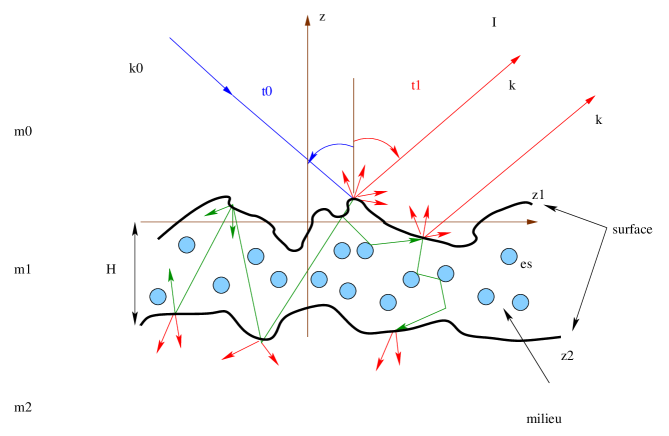
Figure 1: Random medium with rough boundaries.

In the following, we consider harmonic waves with $\rme^{-\rmi\,\omega\,t}$ dependence. For a point source located at $\boldsymbol{r}_{0}=\boldsymbol{x}_{0}+z_{0}\,\hat{\boldsymbol{e}}_{z}$ in the medium $V_{0}$, the field scattered by the rough surfaces and the random medium at the point $\boldsymbol{r}=\boldsymbol{x}+z\,\hat{\boldsymbol{e}}_{z}$ in the media $V_{0}$, $V_{1}$, $V_{2}$ are, respectively, given by the dyadic Green functions [16, 29] $\overline{\boldsymbol{G}}^{00}_{SV}(\boldsymbol{r},\boldsymbol{r}_{0},\omega)$, $\overline{\boldsymbol{G}}^{10}_{SV}(\boldsymbol{r},\boldsymbol{r}_{0},\omega)$, $\overline{\boldsymbol{G}}^{20}_{SV}(\boldsymbol{r},\boldsymbol{r}_{0},\omega)$. Here, for $\overline{\boldsymbol{G}}^{aa_{0}}_{SV}(\boldsymbol{r},\boldsymbol{r}_{0},\omega)$, the upperscripts $a$,$a_{0}$ are, respectively, the receiver location and the source location. These Green functions satisfy [29, 30]:

• Propagation equations :

  $$\nabla\times\nabla\times\overline{\boldsymbol{G}}^{00}_{SV}(\boldsymbol{r},\boldsymbol{r}_{0},\omega)-\epsilon_{0}(\omega)\,K_{vac}^{2}\,\overline{\boldsymbol{G}}^{00}_{SV}(\boldsymbol{r},\boldsymbol{r}_{0},\omega)=\delta(\boldsymbol{r}-\boldsymbol{r}_{0})\,\overline{\boldsymbol{I}}\,,$$ (1)

  $$\nabla\times\nabla\times\overline{\boldsymbol{G}}^{10}_{SV}(\boldsymbol{r},\boldsymbol{r}_{0},\omega)-\epsilon_{V}(\boldsymbol{r},\omega)\,K_{vac}^{2}\,\overline{\boldsymbol{G}}^{10}_{SV}(\boldsymbol{r},\boldsymbol{r}_{0},\omega)=0\,,$$ (2)

  $$\nabla\times\nabla\times\overline{\boldsymbol{G}}^{20}_{SV}(\boldsymbol{r},\boldsymbol{r}_{0},\omega)-\epsilon_{2}(\omega)\,K_{vac}^{2}\,\overline{\boldsymbol{G}}^{20}_{SV}(\boldsymbol{r},\boldsymbol{r}_{0},\omega)=0\,,$$ (3)

  with $K_{vac}\equiv\omega/c_{vac}$ the vacuum wave number, and $c_{vac}$ the light speed in the vacuum. The permittivity $\epsilon_{V}(\boldsymbol{r},\omega)$ inside the random medium $V_{1}$ is defined by :

  $$\epsilon_{V}(\boldsymbol{r},\omega)=\epsilon_{1}(\omega)+\sum_{j=1}^{N}(\epsilon_{s}(\omega)-\epsilon_{1}(\omega))\,\Theta_{s}(\boldsymbol{r}-\boldsymbol{r}_{j})\,,$$ (4)

  where $\boldsymbol{r}_{1},\dots,\boldsymbol{r}_{N}$ are the center of the particles, and $\Theta_{s}$ describes the spherical particle shape :

  $$\Theta_{s}(\boldsymbol{r})=\left\{\begin{array}[]{cc}1&\mbox{if}\quad||\boldsymbol{r}||<r_{s}\\ 0&\mbox{if}\quad||\boldsymbol{r}||>r_{s}\end{array}\right.\,,$$ (5)

  with $r_{s}$ the particle radius.

• Boundary conditions on the upper rough surface:

  $$\hat{\boldsymbol{n}}_{s1}\cdot\epsilon_{0}(\omega)\,\overline{\boldsymbol{G}}^{00}_{SV}(\boldsymbol{r},\boldsymbol{r}_{0},\omega)=\hat{\boldsymbol{n}}_{s1}\cdot\epsilon_{1}(\omega)\,\overline{\boldsymbol{G}}^{10}_{SV}(\boldsymbol{r},\boldsymbol{r}_{0},\omega),$$ (6)

  $$\hat{\boldsymbol{n}}_{s1}\times\overline{\boldsymbol{G}}^{00}_{SV}(\boldsymbol{r},\boldsymbol{r}_{0},\omega)=\hat{\boldsymbol{n}}_{s1}\times\overline{\boldsymbol{G}}^{10}_{SV}(\boldsymbol{r},\boldsymbol{r}_{0},\omega)\,,$$ (7)

  $$\hat{\boldsymbol{n}}_{s1}\cdot\left[\nabla\times\overline{\boldsymbol{G}}^{00}_{SV}(\boldsymbol{r},\boldsymbol{r}_{0},\omega)\right]=\hat{\boldsymbol{n}}_{s1}\cdot\left[\nabla\times\overline{\boldsymbol{G}}^{10}_{SV}(\boldsymbol{r},\boldsymbol{r}_{0},\omega))\right]\,,$$ (8)

  $$\hat{\boldsymbol{n}}_{s1}\times\left[\nabla\times\overline{\boldsymbol{G}}^{00}_{SV}(\boldsymbol{r},\boldsymbol{r}_{0},\omega)\right]=\hat{\boldsymbol{n}}_{s1}\times\,\left[\nabla\times\overline{\boldsymbol{G}}^{10}_{SV}(\boldsymbol{r},\boldsymbol{r}_{0},\omega)\right],$$ (9)

  where $\boldsymbol{r}=\boldsymbol{x}+h_{1}(\boldsymbol{x})\hat{\boldsymbol{e}}_{z}$, and $\hat{\boldsymbol{n}}_{s1}$ is the exterior normal to the rough surface $z=h_{1}(\boldsymbol{x})$:

  $$\hat{\boldsymbol{n}}_{s1}\equiv\frac{\hat{\boldsymbol{e}}_{z}-\nabla h_{1}(\boldsymbol{x})}{(1+(\nabla h_{1}(\boldsymbol{x}))^{2})^{1/2}}\,.$$ (10)

• Boundary conditions on the bottom rough surface :

  $$\hat{\boldsymbol{n}}_{s2}\cdot\epsilon_{1}(\omega)\,\overline{\boldsymbol{G}}^{10}_{SV}(\boldsymbol{r},\boldsymbol{r}_{0},\omega)=\hat{\boldsymbol{n}}_{s2}\cdot\epsilon_{2}(\omega)\,\overline{\boldsymbol{G}}^{20}_{SV}(\boldsymbol{r},\boldsymbol{r}_{0},\omega),$$ (11)

  $$\hat{\boldsymbol{n}}_{s2}\times\overline{\boldsymbol{G}}^{10}_{SV}(\boldsymbol{r},\boldsymbol{r}_{0},\omega)=\hat{\boldsymbol{n}}_{s2}\times\overline{\boldsymbol{G}}^{20}_{SV}(\boldsymbol{r},\boldsymbol{r}_{0},\omega)\,,$$ (12)

  $$\hat{\boldsymbol{n}}_{s2}\cdot\left[\nabla\times\overline{\boldsymbol{G}}^{10}_{SV}(\boldsymbol{r},\boldsymbol{r}_{0},\omega)\right]=\hat{\boldsymbol{n}}_{s2}\cdot\left[\nabla\times\overline{\boldsymbol{G}}^{20}_{SV}(\boldsymbol{r},\boldsymbol{r}_{0},\omega))\right]\,,$$ (13)

  $$\hat{\boldsymbol{n}}_{s2}\times\left[\nabla\times\overline{\boldsymbol{G}}^{10}_{SV}(\boldsymbol{r},\boldsymbol{r}_{0},\omega)\right]=\hat{\boldsymbol{n}}_{s2}\times\,\left[\nabla\times\overline{\boldsymbol{G}}^{20}_{SV}(\boldsymbol{r},\boldsymbol{r}_{0},\omega)\right],$$ (14)

  where $\boldsymbol{r}=\boldsymbol{x}+[-H+h_{2}(\boldsymbol{x})]\hat{\boldsymbol{e}}_{z}$, and $\hat{\boldsymbol{n}}_{s2}$ is the exterior normal to the rough surface $z=h_{2}(\boldsymbol{x})$:

  $$\hat{\boldsymbol{n}}_{s2}\equiv\frac{-\hat{\boldsymbol{e}}_{z}+\nabla h_{2}(\boldsymbol{x})}{(1+(\nabla h_{2}(\boldsymbol{x}))^{2})^{1/2}}\,.$$ (15)

• Radiative conditions at infinity in the media $V_{0}$ and $V_{2}$.

We also use Green functions where the source is situated in the medium $V_{1}$. The fields in the medium $V_{0}$, $V_{1}$, $V_{2}$ are given by the Green functions $\overline{\boldsymbol{G}}^{01}_{SV}(\boldsymbol{r},\boldsymbol{r}_{0},\omega)$, $\overline{\boldsymbol{G}}^{11}_{SV}(\boldsymbol{r},\boldsymbol{r}_{0},\omega)$, $\overline{\boldsymbol{G}}^{21}_{SV}(\boldsymbol{r},\boldsymbol{r}_{0},\omega)$ which verify:

• Propagation equations:

  $$\nabla\times\nabla\times\overline{\boldsymbol{G}}_{SV}^{01}(\boldsymbol{r},\boldsymbol{r}_{0})-\epsilon_{0}(\omega)\,K_{vac}^{2}\,\overline{\boldsymbol{G}}_{SV}^{01}(\boldsymbol{r},\boldsymbol{r}_{0})=0\,,$$ (16)

  $$\nabla\times\nabla\times\overline{\boldsymbol{G}}_{SV}^{11}(\boldsymbol{r},\boldsymbol{r}_{0})-\epsilon_{V}(\boldsymbol{r},\omega)\,K_{vac}^{2}\,\overline{\boldsymbol{G}}_{SV}^{11}(\boldsymbol{r},\boldsymbol{r}_{0})=\delta(\boldsymbol{r}-\boldsymbol{r}_{0})\,\overline{\boldsymbol{I}}\,,$$ (17)

  $$\nabla\times\nabla\times\overline{\boldsymbol{G}}_{SV}^{21}(\boldsymbol{r},\boldsymbol{r}_{0})-\epsilon_{2}(\omega)\,K_{vac}^{2}\,\overline{\boldsymbol{G}}_{SV}^{21}(\boldsymbol{r},\boldsymbol{r}_{0})=0\,,$$ (18)

• Boundary conditions on the upper rough surfaces:

  $$\hat{\boldsymbol{n}}_{s1}\cdot\epsilon_{1}(\omega)\,\overline{\boldsymbol{G}}_{SV}^{11}(\boldsymbol{r},\boldsymbol{r}_{0})=\hat{\boldsymbol{n}}_{s1}\cdot\epsilon_{0}(\omega)\,\overline{\boldsymbol{G}}_{SV}^{01}(\boldsymbol{r},\boldsymbol{r}_{0})\,,$$ (19)

  $$\hat{\boldsymbol{n}}_{s1}\times\overline{\boldsymbol{G}}_{SV}^{11}(\boldsymbol{r},\boldsymbol{r}_{0})=\hat{\boldsymbol{n}}_{s1}\times\overline{\boldsymbol{G}}_{SV}^{01}(\boldsymbol{r},\boldsymbol{r}_{0})\,,$$ (20)

  $$\hat{\boldsymbol{n}}_{s1}\cdot\left[\nabla\times\overline{\boldsymbol{G}}_{SV}^{11}(\boldsymbol{r},\boldsymbol{r}_{0})\right]=\hat{\boldsymbol{n}}_{s1}\cdot\left[\nabla\times\overline{\boldsymbol{G}}_{SV}^{01}(\boldsymbol{r},\boldsymbol{r}_{0})\right]\,,$$ (21)

  $$\hat{\boldsymbol{n}}_{s1}\times\left[\nabla\times\overline{\boldsymbol{G}}_{SV}^{11}(\boldsymbol{r},\boldsymbol{r}_{0})\right]=\hat{\boldsymbol{n}}_{s1}\times\,\left[\nabla\times\overline{\boldsymbol{G}}_{SV}^{01}(\boldsymbol{r},\boldsymbol{r}_{0})\right],$$ (22)

• Boundary conditions on the lower rough surface:

  $$\hat{\boldsymbol{n}}_{s2}\cdot\epsilon_{1}(\omega)\,\overline{\boldsymbol{G}}^{11}_{SV}(\boldsymbol{r},\boldsymbol{r}_{0},\omega)=\hat{\boldsymbol{n}}_{s2}\cdot\epsilon_{2}(\omega)\,\overline{\boldsymbol{G}}^{21}_{SV}(\boldsymbol{r},\boldsymbol{r}_{0},\omega),$$ (23)

  $$\hat{\boldsymbol{n}}_{s2}\times\overline{\boldsymbol{G}}^{11}_{SV}(\boldsymbol{r},\boldsymbol{r}_{0},\omega)=\hat{\boldsymbol{n}}_{s2}\times\overline{\boldsymbol{G}}^{21}_{SV}(\boldsymbol{r},\boldsymbol{r}_{0},\omega)\,,$$ (24)

  $$\hat{\boldsymbol{n}}_{s2}\cdot\left[\nabla\times\overline{\boldsymbol{G}}^{11}_{SV}(\boldsymbol{r},\boldsymbol{r}_{0},\omega)\right]=\hat{\boldsymbol{n}}_{s2}\cdot\left[\nabla\times\overline{\boldsymbol{G}}^{21}_{SV}(\boldsymbol{r},\boldsymbol{r}_{0},\omega))\right]\,,$$ (25)

  $$\hat{\boldsymbol{n}}_{s2}\times\left[\nabla\times\overline{\boldsymbol{G}}^{11}_{SV}(\boldsymbol{r},\boldsymbol{r}_{0},\omega)\right]=\hat{\boldsymbol{n}}_{s2}\times\,\left[\nabla\times\overline{\boldsymbol{G}}^{21}_{SV}(\boldsymbol{r},\boldsymbol{r}_{0},\omega)\right],$$ (26)

• Radiative conditions at infinity in the media 0 and 2.

In order to to separate the contribution from the rough surfaces and the random medium, we introduce the dyadic Green functions $\overline{\boldsymbol{G}}^{00}_{S}(\boldsymbol{r},\boldsymbol{r}_{0},\omega)$, $\overline{\boldsymbol{G}}^{10}_{S}(\boldsymbol{r},\boldsymbol{r}_{0},\omega)$, $\overline{\boldsymbol{G}}^{20}_{S}(\boldsymbol{r},\boldsymbol{r}_{0},\omega)$, $\overline{\boldsymbol{G}}^{01}_{S}(\boldsymbol{r},\boldsymbol{r}_{0},\omega)$, $\overline{\boldsymbol{G}}^{11}_{S}(\boldsymbol{r},\boldsymbol{r}_{0},\omega)$, $\overline{\boldsymbol{G}}^{21}_{S}(\boldsymbol{r},\boldsymbol{r}_{0},\omega)$ which describe the scattering by the layer with the rough boundaries but without the random medium. These functions verify similar propagation equations and boundary conditions as the Green functions $\overline{\boldsymbol{G}}^{aa_{0}}_{SV}(\boldsymbol{r},\boldsymbol{r}_{0},\omega)$, where the permittivity $\epsilon_{V}(\boldsymbol{r},\omega)$ due to the random medium is replaced by an effective permittivity $\epsilon_{e}(\omega)$ in equations (2, 17) and the permittivity $\epsilon_{1}(\omega)$ is replaced by $\epsilon_{e}(\omega)$ in equations (6, 11, 19, 23). This effective permittivity will be determined using the Coherent-Potential Approximation (CPA) with the Quasi-Crystalline Approximation (QCA) [16, 17, 31, 32, 33]. We will show in Section 4 how to write these Green functions with the help of scattering operators, which are common tools in scattering theory by rough surfaces [21].

3 Integral equations

The previous system of differential equations with boundary conditions can be transformed into integral equations [16, 17, 29]. For a source in medium 0, we have

$$\overline{\boldsymbol{G}}_{SV}^{00} = \overline{\boldsymbol{G}}_{S}^{00}+\overline{\boldsymbol{G}}_{S}^{01}\cdot\overline{\boldsymbol{V}}^{11}\cdot\overline{\boldsymbol{G}}_{S}^{10}+\overline{\boldsymbol{G}}_{S}^{01}\cdot\overline{\boldsymbol{V}}^{11}\cdot\overline{\boldsymbol{G}}_{SV}^{11}\cdot\overline{\boldsymbol{V}}^{11}\cdot\overline{\boldsymbol{G}}_{S}^{10}\,,$$ (27)

$$\overline{\boldsymbol{G}}_{SV}^{10} = \overline{\boldsymbol{G}}_{S}^{10}+\overline{\boldsymbol{G}}_{S}^{11}\cdot\overline{\boldsymbol{V}}^{11}\cdot\overline{\boldsymbol{G}}_{S}^{10}+\overline{\boldsymbol{G}}_{S}^{11}\cdot\overline{\boldsymbol{V}}^{11}\cdot\overline{\boldsymbol{G}}_{SV}^{11}\cdot\overline{\boldsymbol{V}}^{11}\cdot\overline{\boldsymbol{G}}_{S}^{10}\,,$$ (28)

$$\overline{\boldsymbol{G}}_{SV}^{20} = \overline{\boldsymbol{G}}_{S}^{20}+\overline{\boldsymbol{G}}_{S}^{21}\cdot\overline{\boldsymbol{V}}^{11}\cdot\overline{\boldsymbol{G}}_{S}^{10}+\overline{\boldsymbol{G}}_{S}^{21}\cdot\overline{\boldsymbol{V}}^{11}\cdot\overline{\boldsymbol{G}}_{SV}^{11}\cdot\overline{\boldsymbol{V}}^{11}\cdot\overline{\boldsymbol{G}}_{S}^{10}\,,$$ (29)

and for a source in the medium 1

$$\overline{\boldsymbol{G}}_{SV}^{01} = \overline{\boldsymbol{G}}_{S}^{01}+\overline{\boldsymbol{G}}_{S}^{01}\cdot\overline{\boldsymbol{V}}^{11}\cdot\overline{\boldsymbol{G}}_{SV}^{11}\,,$$ (30)

$$\overline{\boldsymbol{G}}_{SV}^{11} = \overline{\boldsymbol{G}}_{S}^{11}+\overline{\boldsymbol{G}}_{S}^{11}\cdot\overline{\boldsymbol{V}}^{11}\cdot\overline{\boldsymbol{G}}_{SV}^{11}\,,$$ (31)

$$\overline{\boldsymbol{G}}_{SV}^{21} = \overline{\boldsymbol{G}}_{S}^{21}+\overline{\boldsymbol{G}}_{S}^{21}\cdot\overline{\boldsymbol{V}}^{11}\cdot\overline{\boldsymbol{G}}_{SV}^{11}\,,$$ (32)

with

$$\overline{\boldsymbol{V}}^{11}(\boldsymbol{r},\boldsymbol{r}_{0},\omega) = \delta(\boldsymbol{r}-\boldsymbol{r}_{0})\,\overline{\boldsymbol{V}}^{1}(\boldsymbol{r})\,,$$ (33)

$$\overline{\boldsymbol{V}}^{1}(\boldsymbol{r},\omega) \equiv K^{2}_{vac}(\epsilon_{V}(\boldsymbol{r},\omega)-\epsilon_{e}(\omega))\overline{\boldsymbol{I}}\,,$$ (34)

and the following definition :

$$[\overline{\boldsymbol{A}}\cdot\overline{\boldsymbol{B}}](\boldsymbol{r},\boldsymbol{r}_{0})=\int_{V_{1}}\rmd^{3}\,\boldsymbol{r}_{1}\,\overline{\boldsymbol{A}}(\boldsymbol{r},\boldsymbol{r}_{1})\cdot\overline{\boldsymbol{B}}(\boldsymbol{r}_{1},\boldsymbol{r}_{0})\,.$$ (35)

A direct demonstration of these equations involves integral theorems [34], but it is easier to invoke the uniqueness of the solution and verify a posteriori that the integral equations (27-32) satisfy the propagation equations and the boundary conditions. For example, to demonstrate that equation (17) is verified, we apply the operator $\nabla\times\nabla\times-\epsilon_{e}\,K^{2}_{vac}\overline{\boldsymbol{I}}$ on (31), and using the propagation equation satisfied by $\overline{\boldsymbol{G}}_{S}^{11}$ with the definition in (33-35), we obtain

$$(\nabla\times\nabla\times-\epsilon_{e}\,K^{2}_{vac}\overline{\boldsymbol{I}})\cdot\overline{\boldsymbol{G}}_{SV}^{11}(\boldsymbol{r},\boldsymbol{r}_{0}) =(\nabla\times\nabla\times-\epsilon_{e}\,K^{2}_{vac}\overline{\boldsymbol{I}})\cdot\overline{\boldsymbol{G}}_{S}^{11}(\boldsymbol{r},\boldsymbol{r}_{0})$$

$$\quad+(\nabla\times\nabla\times-\epsilon_{e}\,K^{2}_{vac}\overline{\boldsymbol{I}})\cdot\overline{\boldsymbol{G}}_{S}^{11}\cdot\overline{\boldsymbol{V}}^{11}\cdot\overline{\boldsymbol{G}}_{SV}^{11}(\boldsymbol{r},\boldsymbol{r}_{0})\,,$$

$$=\delta(\boldsymbol{r}-\boldsymbol{r}_{0})\overline{\boldsymbol{I}}+\overline{\boldsymbol{V}}^{11}\cdot\overline{\boldsymbol{G}}_{SV}^{11}(\boldsymbol{r},\boldsymbol{r}_{0})\,,$$

$$=\delta(\boldsymbol{r}-\boldsymbol{r}_{0})\overline{\boldsymbol{I}}+K^{2}_{vac}(\epsilon_{V}(\boldsymbol{r})-\epsilon_{e})\,\overline{\boldsymbol{G}}_{SV}^{11}(\boldsymbol{r},\boldsymbol{r}_{0})\,,$$

which is the propagation equation in (17). By using the same procedure, we show that the propagation equations (1-3, 16-18) and the boundary conditions (7-9, 12-14) and (20-22, 24-26) on the rough surfaces are satisfied. The boundary conditions at infinity in media 0 and 2 are specified by the choice of a retarded Green function for $\overline{\boldsymbol{G}}_{S}^{aa_{0}}$. However, due to the introduction of the effective medium $\epsilon_{e}$, the boundary conditions (6, 11, 19, 23) are not satisfied, and we obtain the following boundary conditions:

$$\hat{\boldsymbol{n}}_{s1}\cdot\epsilon_{e}(\omega)\,\overline{\boldsymbol{G}}^{10}_{SV}(\boldsymbol{r},\boldsymbol{r}_{0},\omega)=\hat{\boldsymbol{n}}_{s1}\cdot\epsilon_{0}(\omega)\,\overline{\boldsymbol{G}}^{00}_{SV}(\boldsymbol{r},\boldsymbol{r}_{0},\omega),$$ (36)

$$\hat{\boldsymbol{n}}_{s2}\cdot\epsilon_{e}(\omega)\,\overline{\boldsymbol{G}}^{10}_{SV}(\boldsymbol{r},\boldsymbol{r}_{0},\omega)=\hat{\boldsymbol{n}}_{s2}\cdot\epsilon_{2}(\omega)\,\overline{\boldsymbol{G}}^{20}_{SV}(\boldsymbol{r},\boldsymbol{r}_{0},\omega),$$ (37)

$$\hat{\boldsymbol{n}}_{s1}\cdot\epsilon_{e}(\omega)\,\overline{\boldsymbol{G}}^{11}_{SV}(\boldsymbol{r},\boldsymbol{r}_{0},\omega)=\hat{\boldsymbol{n}}_{s1}\cdot\epsilon_{0}(\omega)\,\overline{\boldsymbol{G}}^{01}_{SV}(\boldsymbol{r},\boldsymbol{r}_{0},\omega),$$ (38)

$$\hat{\boldsymbol{n}}_{s2}\cdot\epsilon_{e}(\omega)\,\overline{\boldsymbol{G}}^{11}_{SV}(\boldsymbol{r},\boldsymbol{r}_{0},\omega)=\hat{\boldsymbol{n}}_{s2}\cdot\epsilon_{2}(\omega)\,\overline{\boldsymbol{G}}^{21}_{SV}(\boldsymbol{r},\boldsymbol{r}_{0},\omega).$$ (39)

We see that in the left-hand side of equations (36-39), the permittivity is not $\epsilon_{1}(\omega)$, as it must be, but is $\epsilon_{e}(\omega)$. If we had defined the Green function $\overline{\boldsymbol{G}}^{aa_{0}}_{S}$ describing the scattering by a homogeneous medium (with rough boundaries) with the permittivity $\epsilon_{1}$, the problem would not exist. But if we want to use the Coherent-Potential Approximation, we must introduce this effective permittivity. We might go around this problem in changing the definition of the Green function $\overline{\boldsymbol{G}}_{S}^{aa_{0}}$ where a small layer of arbitrary small thickness $h$ with permittivity $\epsilon_{1}$ is added along the rough boundaries. (See Figure (2).) These Green functions verify the boundary conditions (6, 11, 19, 23) where the permittivity $\epsilon_{1}$ is not replaced by $\epsilon_{e}$ due to the added layers along the boundaries. Therefore, with this definition, equations (27-32) verify the boundary conditions (6, 11, 19, 23). However, the propagation equations (2, 17) are not satisfied since the added layers produced new contributions. But as we can choose the layers’ thickness as thin as we want, we can neglect the effect of these layers on the propagation equations.

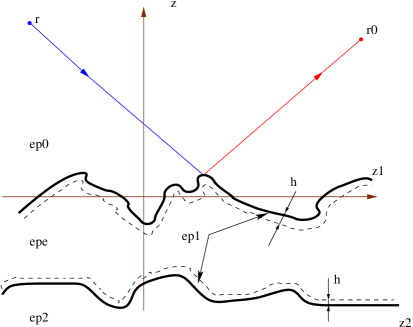
Figure 2: Layers of thickness $h$ with a permittivity $\epsilon_{1}$ around the boundaries .

In the following, we won’t take care of these boundary condition problems, and we will suppose that equations (27-32) are solutions of our problem. The integral equations (27-32) are the key point of our approach. We see that to calculate the field in medium 0 or 2 (when the source is in medium 0) with equations (27) and (29), we first need to determine the Green function $\overline{\boldsymbol{G}}_{SV}^{11}$, where the source and the receiver are in medium 1. This can be done with equation (31) where the only unknown is $\overline{\boldsymbol{G}}_{SV}^{11}$. If the permittivities of the medium 0, 1, and 2 and the effective permittivity were equal ($\epsilon_{e}=\epsilon_{0}=\epsilon_{1}=\epsilon_{2}$), which means that scattering by the boundaries does not take place, the Green function $\overline{\boldsymbol{G}}_{S}^{11}$ will be the Green function in an unbounded medium (A):

$$\overline{\boldsymbol{G}}^{\infty}_{1}(\boldsymbol{r},\boldsymbol{r}_{0})=\left(\overline{\boldsymbol{I}}+\frac{1}{K_{e}^{2}}\nabla\nabla\right)P.V.\frac{\rme^{\rmi\,K_{e}\,||\boldsymbol{r}-\boldsymbol{r}_{0}||}}{4\,\pi\,||\boldsymbol{r}-\boldsymbol{r}_{0}||}\,,$$ (40)

where $K^{2}_{e}=\epsilon_{e}\,\omega^{2}/c^{2}_{vac}$, and equation (31) becomes the usual equation used in scattering theory by random media [17, 34, 35, 36]. In taking into account the boundaries, we have to change this Green function for an infinite random medium by Green functions taking into account the scattering by the boundaries. However, it is worth mentioning that the potential $\overline{\boldsymbol{V}}^{11}$ does not depend on the boundaries, but only on the random medium. Because of this property, we will apply exactly the same procedures developed in scattering theory by an infinite random medium, where the Green function for an unbounded medium must be replaced by Green functions describing scattering by boundaries.

4 Link between the Green functions $\overline{\boldsymbol{G}}_{S}^{11}$ and scattering operator

In this section, we show how to express the Green functions $\overline{\boldsymbol{G}}_{S}^{11}$ with the help of scattering operators which are common tools in scattering theory by rough surfaces [21]. These operators describe the field scattered by a rough surface illuminated by an incident plane wave. (The Green functions $\overline{\boldsymbol{G}}_{S}^{ab}$ describe the same phenomenon for a spherical incident wave.) For a rough surface separating two semi-infinite homogeneous media with permittivities $\epsilon_{0}$ and $\epsilon_{e}$ (Figure 3),

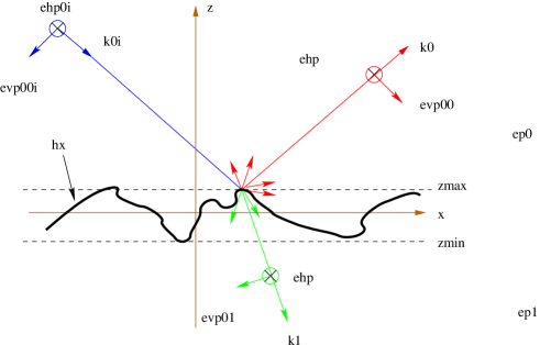
Figure 3: Incident plane wave with wave vector $\boldsymbol{k}_{\boldsymbol{p}_{0}}^{0-}$ reflected into medium 1 with the wave vector $\boldsymbol{k}_{\boldsymbol{p}}^{0+}$ and transmitted into medium 1 with wave vector $\boldsymbol{k}_{\boldsymbol{p}}^{1-}$. The polarization basis are depicted.

the wave equation can be simplified and transformed into the Helmholtz equation :

$$(\Delta+K_{0}^{2})\boldsymbol{E}^{0}(\boldsymbol{r}) =0,\;\;\;z>h(\boldsymbol{x})\,,$$ (41)

$$(\Delta+K_{e}^{2})\boldsymbol{E}^{1}(\boldsymbol{r}) =0,\;\;\;z<h(\boldsymbol{x})\,,$$ (42)

with

$$K_{0}^{2}=\epsilon_{0}\,\left(\frac{\omega}{c_{vac}}\right)^{2}\,,\;\;\;K_{e}^{2}=\epsilon_{e}\,\left(\frac{\omega}{c_{vac}}\right)^{2}\,,$$ (43)

and transversality equation :

$$\nabla\cdot\boldsymbol{E}^{0}(\boldsymbol{x},z) =0,\;\;\;z>h(\boldsymbol{x})\,,$$ (44)

$$\nabla\cdot\boldsymbol{E}^{0}(\boldsymbol{x},z) =0,\;\;\;z<h(\boldsymbol{x})\,.$$ (45)

To find the fields $\boldsymbol{E}^{0}$ and $\boldsymbol{E}^{1}$, we need the boundary conditions on the rough surface $\boldsymbol{r}_{s}=\boldsymbol{x}+h(\boldsymbol{x})\hat{\boldsymbol{e}}_{z}$:

$$\hat{\boldsymbol{n}}_{s}\times\boldsymbol{E}^{0}(\boldsymbol{r}_{s}) = \hat{\boldsymbol{n}}_{s}\times\boldsymbol{E}^{1}(\boldsymbol{r}_{s})\,,$$ (46)

$$\hat{\boldsymbol{n}}_{s}\cdot\epsilon_{0}\,\boldsymbol{E}^{0}(\boldsymbol{r}_{s}) = \hat{\boldsymbol{n}}_{s}\cdot\epsilon_{e}\,\boldsymbol{E}^{1}(\boldsymbol{r}_{s})\,,$$ (47)

$$\hat{\boldsymbol{n}}_{s}\times\left[\nabla\times\boldsymbol{E}^{0}(\boldsymbol{r}_{s})\right] = \hat{\boldsymbol{n}}_{s}\times\left[\nabla\times\boldsymbol{E}^{1}(\boldsymbol{r}_{s})\right]\,,$$ (48)

$$\hat{\boldsymbol{n}}_{s}\cdot\left[\nabla\times\boldsymbol{E}^{0}(\boldsymbol{r}_{s})\right] = \hat{\boldsymbol{n}}_{s}\cdot\left[\nabla\times\boldsymbol{E}^{1}(\boldsymbol{r}_{s})\right]\,,$$ (49)

and the radiation condition at infinity. For an incident plane wave

$$\boldsymbol{E}^{0i}(\boldsymbol{r})=\boldsymbol{E}^{0i}(\boldsymbol{p}_{0})\,\rme^{i\,\boldsymbol{p}_{0}\cdot\boldsymbol{x}-i\,\alpha_{0}(\boldsymbol{p}_{0})z}$$

coming from medium 0, the solution of these equations can be written on the following form [21]:

$$\boldsymbol{E}^{0}(\boldsymbol{x},z)=\boldsymbol{E}^{0i}(\boldsymbol{x},z)+\boldsymbol{E}^{0s}(\boldsymbol{x},z)\,,$$ (50)

$$\boldsymbol{E}^{0s}(\boldsymbol{x},z)=\int\frac{\rmd^{2}\boldsymbol{p}}{(2\pi)^{2}}\,\overline{\boldsymbol{R}}^{10}(\boldsymbol{p}|\boldsymbol{p}_{0})\cdot\boldsymbol{E}^{0\,i}(\boldsymbol{p}_{0})\,\rme^{i\,\boldsymbol{p}\cdot\boldsymbol{x}+i\,\alpha_{0}(\boldsymbol{p})z}\;\;\mbox{for}\;\;z>max_{\boldsymbol{x}}\,h(\boldsymbol{x})\,,$$

(51)

$$\boldsymbol{E}^{1}(\boldsymbol{x},z)=\boldsymbol{E}^{1t}(\boldsymbol{x},z)\,,$$ (52)

$$\boldsymbol{E}^{1t}(\boldsymbol{x},z)=\int\frac{\rmd^{2}\boldsymbol{p}}{(2\pi)^{2}}\,\,\overline{\boldsymbol{T}}^{10}(\boldsymbol{p}|\boldsymbol{p}_{0})\cdot\boldsymbol{E}^{0\,i}(\boldsymbol{p}_{0})\,\rme^{i\,\boldsymbol{p}\cdot\boldsymbol{x}-i\,\alpha_{e}(\boldsymbol{p})z}\;\;\mbox{for}\;\;z<min_{\boldsymbol{x}}\,h(\boldsymbol{x})\,.$$

(53)

Here 

$$\alpha_{0}(\boldsymbol{p})=\sqrt{K_{0}^{2}-\boldsymbol{p}^{2}}\,,\;\;\;\alpha_{e}(\boldsymbol{p})=\sqrt{K_{e}^{2}-\boldsymbol{p}^{2}}\,.$$ (55)

It can be easily checked that the propagation equations (41) and (42) are satisfied with the representations (51,53) and the definitions (55). To satisfy the transversality conditions (44) and (45), we need to decompose the scattering operators $\overline{\boldsymbol{R}}^{10}(\boldsymbol{p}|\boldsymbol{p}_{0})$ and $\overline{\boldsymbol{T}}^{10}(\boldsymbol{p}|\boldsymbol{p}_{0})$ on an orthogonal basis perpendicular to propagation vectors defined by $\boldsymbol{p}$. These vectors are given by the following formula in medium 0 and 1 (Figure 4):

$$\boldsymbol{k}_{\boldsymbol{p}}^{0+} = \boldsymbol{p}+\alpha_{0}(\boldsymbol{p})\hat{\boldsymbol{e}}_{z}\,,$$ (56)

$$\boldsymbol{k}_{\boldsymbol{p}}^{1-} = \boldsymbol{p}-\alpha_{e}(\boldsymbol{p})\hat{\boldsymbol{e}}_{z}\,.$$ (57)

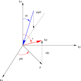
Figure 4: Wave vector decompositions

The basis $[\hat{\boldsymbol{e}}_{V}^{0+}(\boldsymbol{p}),\hat{\boldsymbol{e}}_{H}(\boldsymbol{p})]$ and $[\hat{\boldsymbol{e}}_{V}^{1-}(\boldsymbol{p}),\hat{\boldsymbol{e}}_{H}(\boldsymbol{p})]$ respectively orthogonal to the vectors $\boldsymbol{k}_{\boldsymbol{p}}^{0+}$ and $\boldsymbol{k}_{\boldsymbol{p}}^{1-}$ are then defined by

$$\hat{\boldsymbol{e}}_{H}(\boldsymbol{p}) =\frac{\hat{\boldsymbol{e}}_{z}\times\boldsymbol{k}_{\boldsymbol{p}}^{0\pm}}{||\hat{\boldsymbol{e}}_{z}\times\boldsymbol{k}_{\boldsymbol{p}}^{0\pm}||}=\hat{\boldsymbol{e}}_{z}\times\hat{\boldsymbol{p}}\,,$$ (58)

$$\hat{\boldsymbol{e}}_{V}^{0\pm}(\boldsymbol{p}) =\frac{\hat{\boldsymbol{e}}_{H}(\boldsymbol{p})\times\boldsymbol{k}_{\boldsymbol{p}}^{0\pm}}{||\hat{\boldsymbol{e}}_{H}(\boldsymbol{p}_{0})\times\boldsymbol{k}_{\boldsymbol{p}}^{0\pm}||}=\pm\frac{\alpha_{0}(\boldsymbol{p})}{K_{0}}\hat{\boldsymbol{p}}-\frac{||\boldsymbol{p}||}{K_{0}}\hat{\boldsymbol{e}}_{z}\,,$$ (59)

and

$$\hat{\boldsymbol{e}}_{H}(\boldsymbol{p}) =\frac{\hat{\boldsymbol{e}}_{z}\times\boldsymbol{k}_{\boldsymbol{p}}^{1\pm}}{||\hat{\boldsymbol{e}}_{z}\times\boldsymbol{k}_{\boldsymbol{p}}^{1\pm}||}=\hat{\boldsymbol{e}}_{z}\times\hat{\boldsymbol{p}}\,,$$ (60)

$$\hat{\boldsymbol{e}}_{V}^{1\pm}(\boldsymbol{p}) =\frac{\hat{\boldsymbol{e}}_{H}(\boldsymbol{p})\times\boldsymbol{k}_{\boldsymbol{p}}^{1\pm}}{||\hat{\boldsymbol{e}}_{H}(\boldsymbol{p}_{0})\times\boldsymbol{k}_{\boldsymbol{p}}^{1\pm}||}=\pm\frac{\alpha_{e}(\boldsymbol{p})}{K_{e}}\hat{\boldsymbol{p}}-\frac{||\boldsymbol{p}||}{K_{e}}\hat{\boldsymbol{e}}_{z}\,.$$ (61)

The scattering operators can be written with dyadic notations on these bases:

$$\overline{\boldsymbol{R}}^{10}(\boldsymbol{p}|\boldsymbol{p}_{0})=R^{10}(\boldsymbol{p}|\boldsymbol{p}_{0})_{VV}\,\,\hat{\boldsymbol{e}}^{0+}_{V}(\boldsymbol{p})\hat{\boldsymbol{e}}^{0-}_{V}(\boldsymbol{p}_{0})+R^{10}(\boldsymbol{p}|\boldsymbol{p}_{0})_{HV}\,\,\hat{\boldsymbol{e}}_{H}(\boldsymbol{p})\hat{\boldsymbol{e}}^{0-}_{V}(\boldsymbol{p}_{0})$$

$$+R^{10}(\boldsymbol{p}|\boldsymbol{p}_{0})_{VH}\,\,\hat{\boldsymbol{e}}^{0+}_{V}(\boldsymbol{p})\hat{\boldsymbol{e}}_{H}(\boldsymbol{p}_{0})+R^{10}(\boldsymbol{p}|\boldsymbol{p}_{0})_{HH}\,\,\hat{\boldsymbol{e}}_{H}(\boldsymbol{p})\hat{\boldsymbol{e}}_{H}(\boldsymbol{p}_{0})\,,$$ (62)

$$\overline{\boldsymbol{T}}^{10}(\boldsymbol{p}|\boldsymbol{p}_{0})=T^{10}(\boldsymbol{p}|\boldsymbol{p}_{0})_{VV}\,\,\hat{\boldsymbol{e}}^{1-}_{V}(\boldsymbol{p})\hat{\boldsymbol{e}}^{0-}_{V}(\boldsymbol{p}_{0})+T^{10}(\boldsymbol{p}|\boldsymbol{p}_{0})_{HV}\,\,\hat{\boldsymbol{e}}_{H}(\boldsymbol{p})\hat{\boldsymbol{e}}^{0-}_{V}(\boldsymbol{p}_{0})$$

$$+T^{10}(\boldsymbol{p}|\boldsymbol{p}_{0})_{VH}\,\,\hat{\boldsymbol{e}}^{1-}_{V}(\boldsymbol{p})\hat{\boldsymbol{e}}_{H}(\boldsymbol{p}_{0})+T^{10}(\boldsymbol{p}|\boldsymbol{p}_{0})_{HH}\,\,\hat{\boldsymbol{e}}_{H}(\boldsymbol{p})\hat{\boldsymbol{e}}_{H}(\boldsymbol{p}_{0})\,,$$ (63)

or in a matrix form:

$$\left[\overline{\boldsymbol{R}}^{10}(\boldsymbol{p}|\boldsymbol{p}_{0})\right] =\left(\begin{array}[]{cc}R^{10}(\boldsymbol{p}|\boldsymbol{p}_{0})_{VV}&R^{10}(\boldsymbol{p}|\boldsymbol{p}_{0})_{VH}\\ R^{10}(\boldsymbol{p}|\boldsymbol{p}_{0})_{HV}&R^{10}(\boldsymbol{p}|\boldsymbol{p}_{0})_{HH}\end{array}\right)\,,$$ (66)

$$\left[\overline{\boldsymbol{T}}^{10}(\boldsymbol{p}|\boldsymbol{p}_{0})\right] =\left(\begin{array}[]{cc}T^{10}(\boldsymbol{p}|\boldsymbol{p}_{0})_{VV}&T^{10}(\boldsymbol{p}|\boldsymbol{p}_{0})_{VH}\\ T^{10}(\boldsymbol{p}|\boldsymbol{p}_{0})_{HV}&T^{10}(\boldsymbol{p}|\boldsymbol{p}_{0})_{HH}\end{array}\right)\,.$$ (69)

In a similar way, we can define scattering operators $\overline{\boldsymbol{R}}^{01}$ and $\overline{\boldsymbol{T}}^{01}$ which describe the reflected and transmitted fields when the source is in medium 1 (with permittivity $\epsilon_{e}$). For a rough surface $z=h_{2}(\boldsymbol{x})$ situated on the plane $z=-H$ separating two homogenous media with permittivity $\epsilon_{e}$ and $\ \epsilon_{2}$, we introduce scattering operators $\overline{\boldsymbol{R}}^{H\,21}$ and $\overline{\boldsymbol{T}}^{H\,21}$ which describe the reflected field in medium 1 and the transmitted field in medium 2 when the source is in medium 1 (with the permittivity $\epsilon_{e}$). These scattering operators can be obtained from the scattering operators $\overline{\boldsymbol{R}}^{21}$ and $\overline{\boldsymbol{T}}^{21}$ for a rough surface situated on the plane $z=0$ using the following properties of the scattering operators [21]:

$$\overline{\boldsymbol{R}}^{H\,21}(\boldsymbol{p}|\boldsymbol{p}_{0})=\rme^{\rmi\,(\alpha_{e}(\boldsymbol{p})+\alpha_{e}(\boldsymbol{p}_{0}))H}\,\overline{\boldsymbol{R}}^{21}(\boldsymbol{p}|\boldsymbol{p}_{0})\,,$$ (70)

$$\overline{\boldsymbol{T}}^{H\,21}(\boldsymbol{p}|\boldsymbol{p}_{0})=\rme^{\rmi\,(-\alpha_{2}(\boldsymbol{p})+\alpha_{e}(\boldsymbol{p}_{0}))H}\,\overline{\boldsymbol{T}}^{21}(\boldsymbol{p}|\boldsymbol{p}_{0})\,.$$ (71)

In the rest of this paper, we suppose that we know the scattering operator expressions for $\overline{\boldsymbol{R}}^{10}$, $\overline{\boldsymbol{T}}^{10}$, $\overline{\boldsymbol{R}}^{01}$, $\overline{\boldsymbol{T}}^{01}$, $\overline{\boldsymbol{R}}^{21}$, $\overline{\boldsymbol{T}}^{21}$. Several approximate theories, like the small perturbation [37], the Kirchhoff [20], the small-slope approximation [38], the full-wave method [39], the integral-equation method [7, 40], and others theories [19, 21, 41], can be used to obtain expressions for these operators [21]. With them, we can formally write the scattering operators for a slab with rough boundaries separating two homogeneous media (see Figure 5).

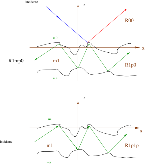
Figure 5: Scattering operator definitions.

We use the following notation $\overline{\boldsymbol{S}}^{\,ab}\left(\boldsymbol{p}\right|\left.\boldsymbol{p}_{0}\right)$ for these scattering operators. The upperscripts $a$ and $b$ indicate the receiver location, the source location and if the waves are upgoing or downgoing. For example, the operator $\overline{\boldsymbol{S}}^{\,\,1+\,0-}\left(\boldsymbol{p}\right|\left.\boldsymbol{p}_{0}\right)$ describes the amplitude of an incident downgoing wave from medium 0 which is scattered into an upgoing wave in medium 1. The upwell electric field in the medium 1 is given by

$$\boldsymbol{E}^{1+}(\boldsymbol{x},z)=\int\frac{\rmd^{2}\boldsymbol{p}}{(2\pi)^{2}}\,\,\rme^{\rmi\,\boldsymbol{p}\cdot\boldsymbol{x}+\rmi\,\alpha_{e}(\boldsymbol{p})z}\,\overline{\boldsymbol{S}}^{\,1+,0-}\left(\boldsymbol{p}\right|\left.\boldsymbol{p}_{0}\right)\cdot\boldsymbol{E}^{0\,i}(\boldsymbol{p}_{0})\,,$$ (72)

and

$$\overline{\boldsymbol{S}}^{\,1+,0-}\left(\boldsymbol{p}\right|\left.\boldsymbol{p}_{0}\right)= S^{1+0-}(\boldsymbol{p}|\boldsymbol{p}_{0})_{VV}\,\,\hat{\boldsymbol{e}}^{1+}_{V}(\boldsymbol{p})\hat{\boldsymbol{e}}^{0-}_{V}(\boldsymbol{p}_{0})+S^{1+0-}(\boldsymbol{p}|\boldsymbol{p}_{0})_{HV}\,\,\hat{\boldsymbol{e}}_{H}(\boldsymbol{p})\hat{\boldsymbol{e}}^{0-}_{V}(\boldsymbol{p}_{0})$$

$$+ S^{1+0-}(\boldsymbol{p}|\boldsymbol{p}_{0})_{VH}\,\,\hat{\boldsymbol{e}}^{1+}_{V}(\boldsymbol{p})\hat{\boldsymbol{e}}_{H}(\boldsymbol{p}_{0})+S^{1+0-}(\boldsymbol{p}|\boldsymbol{p}_{0})_{HH}\,\,\hat{\boldsymbol{e}}_{H}(\boldsymbol{p})\hat{\boldsymbol{e}}_{H}(\boldsymbol{p}_{0})\,.$$ (73)

To express the different operators $\overline{\boldsymbol{S}}^{ab}$ in function of $\overline{\boldsymbol{R}}^{10}$, $\overline{\boldsymbol{T}}^{10}$, $\overline{\boldsymbol{R}}^{01}$, $\overline{\boldsymbol{T}}^{01}$, $\overline{\boldsymbol{R}}^{21}$, $\overline{\boldsymbol{T}}^{21}$, we have just to add formally all the multiple scattering contributions on the rough boundaries ([21], p.24). For example, $\overline{\boldsymbol{S}}^{\,1+\,0-}\left(\boldsymbol{p}\right|\left.\boldsymbol{p}_{0}\right)$ is given by

$$\overline{\boldsymbol{S}}^{1+0-}=\overline{\boldsymbol{R}}^{H\,21}\cdot\overline{\boldsymbol{T}}^{10}+\overline{\boldsymbol{R}}^{H\,21}\cdot\overline{\boldsymbol{R}}^{01}\cdot\overline{\boldsymbol{R}}^{H\,21}\cdot\overline{\boldsymbol{T}}^{10}$$

$$+\overline{\boldsymbol{R}}^{H\,21}\cdot\overline{\boldsymbol{R}}^{01}\cdot\overline{\boldsymbol{R}}^{H\,21}\cdot\overline{\boldsymbol{R}}^{01}\cdot\overline{\boldsymbol{R}}^{H\,21}\cdot\overline{\boldsymbol{T}}^{10}+\dots\,$$ (74)

$$=\overline{\boldsymbol{R}}^{H\,21}\cdot[\overline{\boldsymbol{I}}^{1-1-}_{\perp}-\overline{\boldsymbol{R}}^{01}\cdot\overline{\boldsymbol{R}}^{H\,21}]^{-1}\cdot\overline{\boldsymbol{T}}^{10}\,,$$ (75)

where we have used the following notations:

$$[\overline{\boldsymbol{A}}\cdot\overline{\boldsymbol{B}}](\boldsymbol{p}|\boldsymbol{p}_{0})=\int\frac{\rmd^{2}\boldsymbol{p}_{1}}{(2\pi)^{2}}\,\,\overline{\boldsymbol{A}}(\boldsymbol{p}|\boldsymbol{p}_{1})\cdot\overline{\boldsymbol{B}}(\boldsymbol{p}_{1}|\boldsymbol{p}_{0})\,.$$ (76)

We have defined the projectors $\overline{\boldsymbol{I}}_{\perp}^{1a1a_{0}}$ by

$$\overline{\boldsymbol{I}}^{1a1a_{0}}_{\perp}(\boldsymbol{p}) =\hat{\boldsymbol{e}}_{V}^{1\,a}(\boldsymbol{p})\hat{\boldsymbol{e}}_{V}^{1\,a_{0}}(\boldsymbol{p})+\hat{\boldsymbol{e}}_{H}(\boldsymbol{p})\hat{\boldsymbol{e}}_{H}(\boldsymbol{p})\,,$$ (77)

$$\overline{\boldsymbol{I}}^{1a1a_{0}}_{\perp}(\boldsymbol{p}|\boldsymbol{p}_{0}) =(2\pi)^{2}\,\delta(\boldsymbol{p}-\boldsymbol{p}_{0})\,\overline{\boldsymbol{I}}^{1a1a_{0}}_{\perp}(\boldsymbol{p})\,,$$ (78)

where $a$ and $a_{0}$ are the sign $+$ or $-$. The operator $\overline{\boldsymbol{I}}^{1a1a_{0}}_{\perp}(\boldsymbol{p}|\boldsymbol{p}_{0})$ is the linear identity mapping from the space vector defined by the basis $[\hat{\boldsymbol{e}}_{V}^{1a_{0}}(\boldsymbol{p})$,$\hat{\boldsymbol{e}}_{H}(\boldsymbol{p})]$ to the space vector defined by $[\hat{\boldsymbol{e}}_{V}^{1a}(\boldsymbol{p})$,$\hat{\boldsymbol{e}}_{H}(\boldsymbol{p})]$. To write the electric field $\boldsymbol{E}^{1+}(\boldsymbol{x},z)$ inside the slab with the scattering operator $\overline{\boldsymbol{S}}^{1+0-}$, we have implicitly assumed that the layer is sufficiently thick in order to have the condition $-H+max_{\boldsymbol{x}}h_{2}(\boldsymbol{x})<z<min_{\boldsymbol{x}}h_{1}(\boldsymbol{x})$. Furthermore, we will suppose that all the particles are inside the layer defined by $-H+max_{\boldsymbol{x}}h_{2}(\boldsymbol{x})<z<min_{\boldsymbol{x}}h_{1}(\boldsymbol{x})$. Otherwise, the Rayleigh hypothesis [21] must be invoked to justify the use of the scattering operator for $-H+max_{\boldsymbol{x}}h_{2}(\boldsymbol{x})>z$ and $z>min_{\boldsymbol{x}}h_{1}(\boldsymbol{x})$.

Using the same reasoning for the different contributions, we obtain:

$$\overline{\boldsymbol{S}}^{\,1-\,1-} =[\overline{\boldsymbol{I}}^{1-1-}_{\perp}-\overline{\boldsymbol{R}}^{01}\cdot\overline{\boldsymbol{R}}^{H\,21}]^{-1}-\overline{\boldsymbol{I}}^{1-1-}_{\perp}\,,$$ (79)

$$\overline{\boldsymbol{S}}^{\,1+\,1-} =\overline{\boldsymbol{R}}^{H\,21}\cdot[\overline{\boldsymbol{I}}^{1-1-}_{\perp}+\overline{\boldsymbol{S}}^{\,1-\,1-}]\,,$$ (80)

$$\overline{\boldsymbol{S}}^{\,1-\,1+} =[\overline{\boldsymbol{I}}^{1-1-}_{\perp}+\overline{\boldsymbol{S}}^{\,1-\,1-}]\cdot\overline{\boldsymbol{R}}^{01}\,,$$ (81)

$$\overline{\boldsymbol{S}}^{\,1+\,1+} =[\overline{\boldsymbol{I}}^{1+1+}_{\perp}-\overline{\boldsymbol{R}}^{H\,21}\cdot\overline{\boldsymbol{R}}^{01}]^{-1}-\overline{\boldsymbol{I}}^{1+1+}_{\perp}\,,$$ (82)

$$=\overline{\boldsymbol{R}}^{H\,21}\cdot\overline{\boldsymbol{S}}^{\,1-\,1+}\,,$$ (83)

$$\overline{\boldsymbol{S}}^{\,0+\,0-} =\overline{\boldsymbol{R}}^{10}+\overline{\boldsymbol{T}}^{01}\cdot\overline{\boldsymbol{S}}^{\,1+\,1-}\cdot\overline{\boldsymbol{T}}^{10}\,,$$ (84)

$$\overline{\boldsymbol{S}}^{\,1+\,0-} =\overline{\boldsymbol{S}}^{\,1+\,1-}\cdot\overline{\boldsymbol{T}}^{10}\,,$$ (85)

$$\overline{\boldsymbol{S}}^{\,1-\,0-} =[\overline{\boldsymbol{I}}^{1-1-}_{\perp}+\overline{\boldsymbol{S}}^{\,1-\,1-}]\cdot\overline{\boldsymbol{T}}^{10}\,,$$ (86)

$$\overline{\boldsymbol{S}}^{\,0+\,1-} =\overline{\boldsymbol{T}}^{01}\cdot\overline{\boldsymbol{S}}^{\,1+\,1-}\,,$$ (87)

$$\overline{\boldsymbol{S}}^{\,0+\,1+} =\overline{\boldsymbol{T}}^{01}\cdot[\overline{\boldsymbol{I}}_{\perp}^{1+1+}+\overline{\boldsymbol{S}}^{\,1+\,1+}]\,.$$ (88)

We now show how to express the Green operators $\overline{\boldsymbol{G}}^{aa_{0}}_{S}(\boldsymbol{r},\boldsymbol{r}_{0})$ with the scattering operators $\overline{\boldsymbol{S}}^{\,a\pm\,a_{0}\pm}\left(\boldsymbol{p}\right|\left.\boldsymbol{p}_{0}\right)$.

To determine, for example, the Green operator $\overline{\boldsymbol{G}}_{S}^{1\,1}(\boldsymbol{r},\boldsymbol{r}_{0})$, we have to calculate the field produced inside the slab by a spherical source which is also in medium 1. We can decompose the function $\overline{\boldsymbol{G}}_{S}^{1\,1}(\boldsymbol{r},\boldsymbol{r}_{0})$ under the following form:

$$\overline{\boldsymbol{G}}_{S}^{1\,1}(\boldsymbol{r},\boldsymbol{r}_{0})=\overline{\boldsymbol{G}}_{1}^{\,\infty}(\boldsymbol{r},\boldsymbol{r}_{0})+\overline{\boldsymbol{G}}_{S}^{1+\,1+}(\boldsymbol{r},\boldsymbol{r}_{0})$$

$$+\overline{\boldsymbol{G}}_{S}^{1+\,1-}(\boldsymbol{r},\boldsymbol{r}_{0})+\overline{\boldsymbol{G}}_{S}^{1-\,1-}(\boldsymbol{r},\boldsymbol{r}_{0})+\overline{\boldsymbol{G}}_{S}^{1-\,1+}(\boldsymbol{r},\boldsymbol{r}_{0})\,.$$ (89)

The first term is the spherical source term in an infinite homogeneous medium (with permittivity $\epsilon_{e}$), and the following terms are the fields produced by multiple scattering process on the rough boundaries. We can obtain these contributions noticing that the source term

$$\overline{\boldsymbol{G}}_{1}^{\,\infty}(\boldsymbol{r},\boldsymbol{r}_{0})=\left(\overline{\boldsymbol{I}}+\frac{1}{K_{e}^{2}}\nabla\nabla\right)P.V.\frac{\rme^{\rmi\,K_{e}\,||\boldsymbol{r}-\boldsymbol{r}_{0}||}}{4\,\pi\,||\boldsymbol{r}-\boldsymbol{r}_{0}||}\,$$

can be decomposed as a linear combination of plane wave using the Weyl formula (A):

$$\mbox{for}\quad z>z_{0}:$$

$$\overline{\boldsymbol{G}}_{1}^{\,\infty}(\boldsymbol{r},\boldsymbol{r}_{0})=\frac{\rmi}{2}\,\int\frac{\rmd^{2}\boldsymbol{p}_{0}}{(2\pi)^{2}}\,\rme^{\rmi\,\boldsymbol{p}_{0}\cdot(\boldsymbol{x}-\boldsymbol{x}_{0})+\rmi\,\alpha_{e}(\boldsymbol{p}_{0})\,(z-z_{0})}\,(\overline{\boldsymbol{I}}-\hat{\boldsymbol{k}}^{1\,+}_{\boldsymbol{p}_{0}}\hat{\boldsymbol{k}}^{1\,+}_{\boldsymbol{p}_{0}})\,\frac{1}{\alpha_{e}(\boldsymbol{p}_{0})}\,;$$ (90)

$$\mbox{for}\quad z<z_{0}:$$

$$\overline{\boldsymbol{G}}_{1}^{\,\infty}(\boldsymbol{r},\boldsymbol{r}_{0})=\frac{\rmi}{2}\,\int\frac{\rmd^{2}\boldsymbol{p}_{0}}{(2\pi)^{2}}\,\rme^{\rmi\,\boldsymbol{p}_{0}\cdot(\boldsymbol{x}-\boldsymbol{x}_{0})-\rmi\,\alpha_{e}(\boldsymbol{p}_{0})\,(z-z_{0})}\,(\overline{\boldsymbol{I}}-\hat{\boldsymbol{k}}^{1\,-}_{\boldsymbol{p}_{0}}\hat{\boldsymbol{k}}^{1\,-}_{\boldsymbol{p}_{0}})\,\frac{1}{\alpha_{e}(\boldsymbol{p}_{0})}\,,$$ (91)

with $\boldsymbol{k}^{1\,\pm}_{\boldsymbol{p}_{0}}=\boldsymbol{p}_{0}\pm\alpha_{e}(\boldsymbol{p}_{0})\,\hat{\boldsymbol{e}}_{z}$ and $\hat{\boldsymbol{k}}^{1\,\pm}_{\boldsymbol{p}_{0}}=\boldsymbol{k}^{1\,\pm}_{\boldsymbol{p}_{0}}/||\boldsymbol{k}^{1\,\pm}_{\boldsymbol{p}_{0}}||$. Hence, for $z\neq z_{0}$, $\overline{\boldsymbol{G}}_{1}^{\,\infty}$ is a linear combination of the following plane waves:

$$\frac{\rmi}{2\,\alpha_{e}(\boldsymbol{p}_{0})}\,\rme^{\rmi\,\hat{\boldsymbol{k}}^{1\,\pm}_{\boldsymbol{p}_{0}}\cdot(\boldsymbol{r}-\boldsymbol{r}_{0})}(\overline{\boldsymbol{I}}-\hat{\boldsymbol{k}}^{1\,\pm}_{\boldsymbol{p}_{0}}\hat{\boldsymbol{k}}^{1\,\pm}_{\boldsymbol{p}_{0}})\,,$$ (92)

which are transverse to the propagation directions $\hat{\boldsymbol{k}}^{1\,\pm}_{\boldsymbol{p}_{0}}$ because $(\overline{\boldsymbol{I}}-\hat{\boldsymbol{k}}^{1\,\pm}_{\boldsymbol{p}_{0}}\hat{\boldsymbol{k}}^{1\,\pm}_{\boldsymbol{p}_{0}})\cdot\hat{\boldsymbol{k}}^{1\,\pm}_{\boldsymbol{p}_{0}}=0$. For each of these plane waves, we can calculate the field produced by the scattering process on the boundaries with the scattering operators $\overline{\boldsymbol{S}}^{\,1\times\,1\times}$. By using the superposition principle of the electric field [42], we have for the contribution due to $\overline{\boldsymbol{S}}^{1+\,1-}$:

$$\overline{\boldsymbol{G}}_{S}^{1+\,1-}(\boldsymbol{r},\boldsymbol{r}_{0})=\frac{\rmi}{2}\int\!\!\!\int\frac{\rmd^{2}\boldsymbol{p}}{(2\pi)^{2}}\frac{\rmd^{2}\boldsymbol{p}_{0}}{(2\pi)^{2}}\, \rme^{\rmi\,\boldsymbol{p}\cdot\boldsymbol{x}-\rmi\,\boldsymbol{p}_{0}\cdot\boldsymbol{x}_{0}+\rmi\,\alpha_{e}(\boldsymbol{p})\,z+\rmi\,\alpha_{e}(\boldsymbol{p}_{0})\,z_{0}}$$

$$\times\overline{\boldsymbol{S}}^{\,1+\,1-}\left(\boldsymbol{p}\right|\left.\boldsymbol{p}_{0}\right)\cdot(\overline{\boldsymbol{I}}-\hat{\boldsymbol{k}}^{1\,-}_{\boldsymbol{p}_{0}}\hat{\boldsymbol{k}}^{1\,-}_{\boldsymbol{p}_{0}})\,\frac{1}{\alpha_{e}(\boldsymbol{p}_{0})}\,,$$

since in this case, the incident waves are propagating along the direction $\hat{\boldsymbol{k}}^{1\,-}_{\boldsymbol{p}_{0}}$. We summarize all the contributions (89) to $\overline{\boldsymbol{G}}_{S}^{1\,1}$ under the form:

$$\overline{\boldsymbol{G}}_{S}^{1\,1}(\boldsymbol{r},\boldsymbol{r}_{0})=\overline{\boldsymbol{G}}_{1}^{\,\infty}(\boldsymbol{r},\boldsymbol{r}_{0})+\sum_{a,a_{0}=\pm}\overline{\boldsymbol{G}}_{S}^{1a\,1a_{0}}(\boldsymbol{r},\boldsymbol{r}_{0})\,,$$

(94)

with

$$\overline{\boldsymbol{G}}_{S}^{1a\,1a_{0}}(\boldsymbol{r},\boldsymbol{r}_{0})=\frac{\rmi}{2}\int\!\!\!\int\frac{\rmd^{2}\boldsymbol{p}}{(2\pi)^{2}}\frac{\rmd^{2}\boldsymbol{p}_{0}}{(2\pi)^{2}}\, \rme^{\rmi\,\boldsymbol{p}\cdot\boldsymbol{x}-\rmi\,\boldsymbol{p}_{0}\cdot\boldsymbol{x}_{0}+a\,\rmi\,\alpha_{e}(\boldsymbol{p})\,z-a_{0}\,\rmi\,\alpha_{e}(\boldsymbol{p}_{0})\,z_{0}}$$

$$\times\overline{\boldsymbol{S}}^{\,1a\,1a_{0}}\left(\boldsymbol{p}\right|\left.\boldsymbol{p}_{0}\right)\cdot(\overline{\boldsymbol{I}}-\hat{\boldsymbol{k}}^{1\,a_{0}}_{\boldsymbol{p}_{0}}\hat{\boldsymbol{k}}^{1\,a_{0}}_{\boldsymbol{p}_{0}})\frac{1}{\alpha_{e}(\boldsymbol{p}_{0})}\,.$$

where $a$, $a_{0}$ are the sign $+$ or $-$. By using the same arguments, we demonstrate that:

$$\overline{\boldsymbol{G}}_{S}^{10}(\boldsymbol{r},\boldsymbol{r}_{0})=\overline{\boldsymbol{G}}_{S}^{1+\,0-}(\boldsymbol{r},\boldsymbol{r}_{0})+\overline{\boldsymbol{G}}_{S}^{1-\,0-}(\boldsymbol{r},\boldsymbol{r}_{0})\,,$$ (96)

$$\overline{\boldsymbol{G}}_{S}^{01}(\boldsymbol{r},\boldsymbol{r}_{0})=\overline{\boldsymbol{G}}_{S}^{0+\,1+}(\boldsymbol{r},\boldsymbol{r}_{0})+\overline{\boldsymbol{G}}_{S}^{0+\,1-}(\boldsymbol{r},\boldsymbol{r}_{0})\,,$$ (97)

$$\overline{\boldsymbol{G}}_{S}^{00}(\boldsymbol{r},\boldsymbol{r}_{0})=\overline{\boldsymbol{G}}_{0}^{\,\infty}(\boldsymbol{r},\boldsymbol{r}_{0})+\overline{\boldsymbol{G}}_{S}^{0+\,0-}(\boldsymbol{r},\boldsymbol{r}_{0})\,,$$ (98)

with

$$\overline{\boldsymbol{G}}_{S}^{1a\,0-}(\boldsymbol{r},\boldsymbol{r}_{0})=\frac{\rmi}{2}\int\!\!\!\int\frac{\rmd^{2}\boldsymbol{p}}{(2\pi)^{2}}\frac{\rmd^{2}\boldsymbol{p}_{0}}{(2\pi)^{2}}\, \rme^{\rmi\,\boldsymbol{p}\cdot\boldsymbol{x}-\rmi\,\boldsymbol{p}_{0}\cdot\boldsymbol{x}_{0}+a\,\rmi\,\alpha_{e}(\boldsymbol{p})\,z+\,\rmi\,\alpha_{0}(\boldsymbol{p}_{0})\,z_{0}}$$

$$\times\overline{\boldsymbol{S}}^{\,1a\,0-}\left(\boldsymbol{p}\right|\left.\boldsymbol{p}_{0}\right)\cdot(\overline{\boldsymbol{I}}-\hat{\boldsymbol{k}}^{0\,-}_{\boldsymbol{p}_{0}}\hat{\boldsymbol{k}}^{0\,-}_{\boldsymbol{p}_{0}})\frac{1}{\alpha_{0}(\boldsymbol{p}_{0})}\,,$$

$$\overline{\boldsymbol{G}}_{S}^{0+\,1a_{0}}(\boldsymbol{r},\boldsymbol{r}_{0})=\frac{\rmi}{2}\int\!\!\!\int\frac{\rmd^{2}\boldsymbol{p}}{(2\pi)^{2}}\frac{\rmd^{2}\boldsymbol{p}_{0}}{(2\pi)^{2}}\, \rme^{\rmi\,\boldsymbol{p}\cdot\boldsymbol{x}-\rmi\,\boldsymbol{p}_{0}\cdot\boldsymbol{x}_{0}+\rmi\,\alpha_{0}(\boldsymbol{p})\,z-a_{0}\,\rmi\,\alpha_{e}(\boldsymbol{p}_{0})\,z_{0}}$$

$$\times\overline{\boldsymbol{S}}^{\,0+\,1a_{0}}\left(\boldsymbol{p}\right|\left.\boldsymbol{p}_{0}\right)\cdot(\overline{\boldsymbol{I}}-\hat{\boldsymbol{k}}^{1\,a_{0}}_{\boldsymbol{p}_{0}}\hat{\boldsymbol{k}}^{1\,a_{0}}_{\boldsymbol{p}_{0}})\frac{1}{\alpha_{e}(\boldsymbol{p}_{0})}\,,$$

$$\overline{\boldsymbol{G}}_{S}^{0+\,0-}(\boldsymbol{r},\boldsymbol{r}_{0})=\frac{\rmi}{2}\int\!\!\!\int\frac{\rmd^{2}\boldsymbol{p}}{(2\pi)^{2}}\frac{\rmd^{2}\boldsymbol{p}_{0}}{(2\pi)^{2}}\, \rme^{\rmi\,\boldsymbol{p}\cdot\boldsymbol{x}-\rmi\,\boldsymbol{p}_{0}\cdot\boldsymbol{x}_{0}+\,\rmi\,\alpha_{0}(\boldsymbol{p})\,z+\,\rmi\,\alpha_{0}(\boldsymbol{p}_{0})\,z_{0}}$$

$$\times\overline{\boldsymbol{S}}^{\,0+\,0-}\left(\boldsymbol{p}\right|\left.\boldsymbol{p}_{0}\right)\cdot(\overline{\boldsymbol{I}}-\hat{\boldsymbol{k}}^{0\,-}_{\boldsymbol{p}_{0}}\hat{\boldsymbol{k}}^{0\,-}_{\boldsymbol{p}_{0}})\frac{1}{\alpha_{0}(\boldsymbol{p}_{0})}\,.$$

5 Lipmann-Schwinger equations and scattered field

If we iterate equation (31), we obtain the following series for the function $\overline{\boldsymbol{G}}_{SV}^{11}$:

$$\overline{\boldsymbol{G}}_{SV}^{11} =\overline{\boldsymbol{G}}_{S}^{11}+\overline{\boldsymbol{G}}_{S}^{11}\cdot\overline{\boldsymbol{V}}^{11}\cdot\overline{\boldsymbol{G}}_{SV}^{11}\,,$$

$$=\overline{\boldsymbol{G}}_{S}^{11}+\overline{\boldsymbol{G}}_{S}^{11}\cdot\overline{\boldsymbol{V}}^{11}\cdot\overline{\boldsymbol{G}}_{S}^{11}+\overline{\boldsymbol{G}}_{S}^{11}\cdot\overline{\boldsymbol{V}}^{11}\cdot\overline{\boldsymbol{G}}_{S}^{11}\cdot\overline{\boldsymbol{V}}^{11}\cdot\overline{\boldsymbol{G}}_{S}^{11}+\dots\,$$

If we introduce the transition operator $\overline{\boldsymbol{T}}_{SV}^{11}$ by

$$\overline{\boldsymbol{G}}_{SV}^{11}=\overline{\boldsymbol{G}}_{S}^{11}+\overline{\boldsymbol{G}}_{S}^{11}\cdot\overline{\boldsymbol{T}}_{SV}^{11}\cdot\overline{\boldsymbol{G}}_{S}^{11}\,,$$ (104)

we obtain Lipmann-Schwinger equations in comparing the definition in (104) with the development in (LABEL:Lip2bis2):

$$\overline{\boldsymbol{T}}_{SV}^{11} =\overline{\boldsymbol{V}}^{11}+\overline{\boldsymbol{V}}^{11}\cdot\overline{\boldsymbol{G}}_{S}^{11}\cdot\overline{\boldsymbol{T}}_{SV}^{11}\,,$$ (105)

$$\overline{\boldsymbol{T}}_{SV}^{11} =\overline{\boldsymbol{V}}^{11}+\overline{\boldsymbol{T}}^{11}_{SV}\cdot\overline{\boldsymbol{G}}_{S}^{11}\cdot\overline{\boldsymbol{V}}^{11}\,.$$ (106)

With these operators, we can straightforwdly rewrite in a compact form equations (27-32):

$$\overline{\boldsymbol{G}}_{SV}^{00} =\overline{\boldsymbol{G}}_{S}^{00}+\overline{\boldsymbol{G}}_{S}^{01}\cdot\overline{\boldsymbol{T}}_{SV}^{11}\cdot\overline{\boldsymbol{G}}_{S}^{10}\,,$$ (107)

$$\overline{\boldsymbol{G}}_{SV}^{10} =\overline{\boldsymbol{G}}_{S}^{10}+\overline{\boldsymbol{G}}_{S}^{11}\cdot\overline{\boldsymbol{T}}_{SV}^{11}\cdot\overline{\boldsymbol{G}}_{S}^{10}\,,$$ (108)

$$\overline{\boldsymbol{G}}_{SV}^{20} =\overline{\boldsymbol{G}}_{S}^{20}+\overline{\boldsymbol{G}}_{S}^{21}\cdot\overline{\boldsymbol{T}}_{SV}^{11}\cdot\overline{\boldsymbol{G}}_{S}^{10}\,,$$ (109)

$$\overline{\boldsymbol{G}}_{SV}^{01} =\overline{\boldsymbol{G}}_{S}^{01}+\overline{\boldsymbol{G}}_{S}^{01}\cdot\overline{\boldsymbol{T}}_{SV}^{11}\cdot\overline{\boldsymbol{G}}_{S}^{11}\,,$$ (110)

$$\overline{\boldsymbol{G}}_{SV}^{21} =\overline{\boldsymbol{G}}_{S}^{21}+\overline{\boldsymbol{G}}_{S}^{21}\cdot\overline{\boldsymbol{T}}_{SV}^{11}\cdot\overline{\boldsymbol{G}}_{S}^{11}\,.$$ (111)

All the scattering processes in the random medium are contained in the transition operator $\overline{\boldsymbol{T}}^{11}_{SV}$. If we know this operator, then we can calculate all the fields in the different media using (107-111). Furthermore, for any source $\boldsymbol{j}_{source}$ in the medium 0, the incident electric field is

$$\boldsymbol{E}^{0i}(\boldsymbol{r}) =\rmi\,\omega\,\mu_{vac}\int\rmd^{3}\boldsymbol{r}_{0}\,\overline{\boldsymbol{G}}_{0}^{\infty}(\boldsymbol{r},\boldsymbol{r}_{0})\cdot\boldsymbol{j}_{source}(\boldsymbol{r}_{0})\,,$$ (112)

where $\mu_{vac}$ is the vacuum permeability. The resulting field in medium 0 is given from (107) and (98) by

$$\boldsymbol{E}_{SV}^{0} =\boldsymbol{E}^{0i}+\boldsymbol{E}^{0s}_{SV}\,,$$ (113)

$$\boldsymbol{E}^{0s}_{SV} =\boldsymbol{E}^{0s}_{S}+\overline{\boldsymbol{G}}_{S}^{01}\cdot\overline{\boldsymbol{T}}^{11}_{SV}\cdot\boldsymbol{E}_{S}^{1\,t}\,,$$ (114)

where

$$\boldsymbol{E}_{S}^{0s}(\boldsymbol{r}) =\rmi\,\omega\,\mu_{vac}\int\rmd^{3}\boldsymbol{r}_{0}\,\overline{\boldsymbol{G}}_{S}^{0+0-}(\boldsymbol{r},\boldsymbol{r}_{0})\cdot\boldsymbol{j}_{source}(\boldsymbol{r}_{0})\,,$$ (115)

$$\boldsymbol{E}_{S}^{1\,t}(\boldsymbol{r}) =\rmi\,\omega\,\mu_{vac}\int\rmd^{3}\boldsymbol{r}_{0}\,\overline{\boldsymbol{G}}_{S}^{10}(\boldsymbol{r},\boldsymbol{r}_{0})\cdot\boldsymbol{j}_{source}(\boldsymbol{r}_{0})\,.$$ (116)

The field $\boldsymbol{E}_{SV}^{0s}$ is the scattered field produced by the random medium and the rough boundaries which is decomposed in two contributions where $\boldsymbol{E}_{S}^{0s}(\boldsymbol{r})$ is the reflected field produced by an homogeneous slab (with permittivity $\epsilon_{e}$) with rough boundaries, and the second term $\overline{\boldsymbol{G}}_{S}^{01}\cdot\overline{\boldsymbol{T}}^{11}_{SV}\cdot\boldsymbol{E}_{S}^{1\,t}$ is the field scattered by the random medium and the rough surfaces. Vector $\boldsymbol{E}_{S}^{1\,t}$ is the transmitted field in medium 1 before any scattering by the particles.

6 Ensemble average

In order to calculate the coherent field reflected by the random slab, we need to define the averaging procedure. Let $<\cdots>_{S}$ and $<\cdots>_{V}$ denote, respectively, the ensemble average over the surfaces and the volume disorder. We also denote $\ll\cdots\gg_{SV}$ the average over the rough surfaces and the volume disorder. We suppose that the rough surfaces and random medium properties are statistically independent, which means that $\ll\cdots\gg_{SV}=<[<\cdots>_{S}]>_{V}=<[<\cdots>_{V}]>_{S}$. In the following development, we won’t use any specific statistical properties of the rough surfaces (except that $<h_{1}(\boldsymbol{x})>_{S}=<h_{2}(\boldsymbol{x})>_{S}=0$); thus, we don’t need to specify them. An extensive description can be found in the references [19, 43]. The ensemble average over the random medium is defined by

$$<f>_{V}=\int_{V_{1}}\rmd^{3}\boldsymbol{r}_{1}\dots\rmd^{3}\boldsymbol{r}_{N}\,\,f(\boldsymbol{r}_{1},\dots,\boldsymbol{r}_{N})\,p(\boldsymbol{r}_{1},\dots,\boldsymbol{r}_{N})\,,$$ (117)

where $\boldsymbol{r}_{1},\cdots,\boldsymbol{r}_{N}$ are the particles positions, and $p(\boldsymbol{r}_{1},\dots,\boldsymbol{r}_{N})$ is the probability density function of finding the N particles at positions $\boldsymbol{r}_{1},\cdots,\boldsymbol{r}_{N}$. We will use a decomposition of this density function with conditional probabilities [16, 17]:

$$p(\boldsymbol{r}_{1},\dots,\boldsymbol{r}_{N})=p(\boldsymbol{r}_{i})p(\boldsymbol{r}_{1},\cdots,\widehat{\boldsymbol{r}_{i}},\cdots\boldsymbol{r}_{N}|\boldsymbol{r}_{i})\,,$$ (118)

$$p(\boldsymbol{r}_{1},\dots,\boldsymbol{r}_{N})=p(\boldsymbol{r}_{i})p(\boldsymbol{r}_{j}|\boldsymbol{r}_{i})p(\boldsymbol{r}_{1},\cdots,\widehat{\boldsymbol{r}_{i}},\cdots\widehat{\boldsymbol{r}_{j}},\cdots,\boldsymbol{r}_{N}|\boldsymbol{r}_{i},\boldsymbol{r}_{j})\,,$$ (119)

where the hat $\,\widehat{}\,$ indicates that the term is absent. The function $p(\boldsymbol{r}_{i})$ is the probability density function of finding a particle at $\boldsymbol{r}_{i}$, $p(\boldsymbol{r}_{i}|\boldsymbol{r}_{j})$ is the conditional probability of finding a particle at $\boldsymbol{r}_{i}$ given a particle at $\boldsymbol{r}_{j}$, etc. If the particles are uniformly distributed inside the random medium $V_{1}$, then the single particle density function is $p(\boldsymbol{r}_{i})=1/\mathcal{V}_{1}$, where $\mathcal{V}_{1}$ is the volume of the area $V_{1}$. In this case, we also define a pair-distribution function by

$$g(||\boldsymbol{r}_{i}-\boldsymbol{r}_{j}||)=p(\boldsymbol{r}_{i}|\boldsymbol{r}_{j})/p(\boldsymbol{r}_{i})\,,$$ (120)

which depends only on the distance between the two particles if we suppose that the distribution of the particles is statistically homogeneous and isotropic. The normalization factor $\mathcal{V}_{1}$ is chosen in such a way that when the particles located at $\boldsymbol{r}_{i}$, $\boldsymbol{r}_{j}$ are far away from each over, their positions are uncorrelated (i.e., $p(\boldsymbol{r}_{i}|\boldsymbol{r}_{j})=p(\boldsymbol{r}_{i})$), and we have

$$\lim_{||\boldsymbol{r}_{i}-\boldsymbol{r}_{j}||\to+\infty}g(||\boldsymbol{r}_{i}-\boldsymbol{r}_{j}||)=1\,.$$ (121)

With these conditional probability functions, we define conditional averages:

$$<f>_{V;\boldsymbol{r}_{i}}=\int_{V_{1}}\rmd^{3}\boldsymbol{r}_{1}\dots\widehat{\rmd^{3}\boldsymbol{r}_{i}}\dots\rmd^{3}\boldsymbol{r}_{N}\,\,f(\boldsymbol{r}_{1},\dots,\boldsymbol{r}_{i},\dots,\boldsymbol{r}_{N})\,$$

$$\times p(\boldsymbol{r}_{1},\dots,\widehat{\boldsymbol{r}_{i}},\dots\boldsymbol{r}_{N}|\boldsymbol{r}_{i})\,,$$ (122)

$$<f>_{V;\boldsymbol{r}_{i},\boldsymbol{r}_{j}}=\int_{V_{1}}\rmd^{3}\boldsymbol{r}_{1}\dots\widehat{\rmd^{3}\boldsymbol{r}_{i}}\dots\widehat{\rmd^{3}\boldsymbol{r}_{j}}\dots\rmd^{3}\boldsymbol{r}_{N}\,\,f(\boldsymbol{r}_{1},\dots,\boldsymbol{r}_{i},\dots,\boldsymbol{r}_{j},\dots,\boldsymbol{r}_{N})\,$$ (123)

$$\times\,p(\boldsymbol{r}_{1},\dots,\widehat{\boldsymbol{r}_{i}},\dots,\widehat{\boldsymbol{r}_{j}},\dots,\boldsymbol{r}_{N}|\boldsymbol{r}_{i},\boldsymbol{r}_{j})\,.$$ (124)

7 Coherent potential approximation and effective medium theory

Until now, we have not clarified how to determine the effective permittivity $\epsilon_{e}(\omega)$. To determine $\epsilon_{e}(\omega)$, we use the fact that under some assumptions (mainly that the effective medium is not spatially dispersive [27] i.e., $\epsilon(\omega,\boldsymbol{k})=\epsilon(\omega)$), it can be shown, using a diagrammatic technique, that the coherent part of the field $<\overline{\boldsymbol{E}}>_{V}$ which propagates inside an infinite random medium behaves as a wave in an homogeneous medium with a renormalized effective permittivity [16, 17, 27, 28, 23, 44, 45]. In order to insure this result in a self-consistent way, we introduce the Coherent Potential Approximation (CPA), which postulates that [16, 17, 27, 31, 33]

$$<\overline{\boldsymbol{G}}_{SV}^{11}>_{V}=\overline{\boldsymbol{G}}_{S}^{11}\,.$$ (125)

This equation is in fact the definition of our effective permittivity $\epsilon_{e}$ and is a generalization of the classical (CPA) approach since we take into account the boundaries in the Green function definitions. Using equation (104), we immediately see that condition (125) is equivalent to

$$<\overline{\boldsymbol{T}}_{SV}^{11}>_{V}=\overline{\boldsymbol{0}}\,,$$ (126)

where

$$\overline{\boldsymbol{T}}_{SV}^{11}=\overline{\boldsymbol{V}}^{11}+\overline{\boldsymbol{V}}^{11}\cdot\overline{\boldsymbol{G}}_{S}^{11}\cdot\overline{\boldsymbol{T}}_{SV}^{11}\,.$$ (127)

Therefore, equations (126, 127) provide a closed system of equations on the unknown $\epsilon_{e}(\omega)$ which takes place in the definition of $\overline{\boldsymbol{V}}^{11}$ and $\overline{\boldsymbol{G}}_{S}^{11}$. Because the random medium is made with spherical particles, it is convenient to express equation (127) as a function of the scattering operator $\overline{\boldsymbol{t}}^{11}_{\boldsymbol{r}_{i}}$ for one particle located at $\boldsymbol{r}_{i}$ in a infinite medium (B). It is defined by

$$\overline{\boldsymbol{t}}^{11}_{\boldsymbol{r}_{i}}=[\overline{\boldsymbol{I}}-\overline{\boldsymbol{v}}^{11}_{\boldsymbol{r}_{i}}\cdot\overline{\boldsymbol{G}}_{1}^{\infty}]^{-1}\cdot\overline{\boldsymbol{v}}^{11}_{\boldsymbol{r}_{i}}\,,$$ (128)

where the scattering potential $\overline{\boldsymbol{v}}^{11}_{\boldsymbol{r}_{i}}$ is:

$$\overline{\boldsymbol{v}}^{11}_{\boldsymbol{r}_{i}}(\boldsymbol{r},\boldsymbol{r}_{0}) = (2\pi)^{2}\,\delta(\boldsymbol{r}-\boldsymbol{r}_{0})\overline{\boldsymbol{v}}^{1}_{\boldsymbol{r}_{i}}(\boldsymbol{r})\,,$$ (129)

$$\overline{\boldsymbol{v}}^{1}_{\boldsymbol{r}_{i}}(\boldsymbol{r}) = K_{vac}^{2}(\epsilon_{s}-\epsilon_{1})\Theta_{s}(\boldsymbol{r}-\boldsymbol{r}_{i})\overline{\boldsymbol{I}}\,.$$ (130)

In order to write equation (127) with the operators $\overline{\boldsymbol{t}}^{11}_{\boldsymbol{r}_{i}}$, following the Korringa demonstration [33], we decompose

$$\overline{\boldsymbol{V}}^{11}(\boldsymbol{r},\boldsymbol{r}_{0})=(2\pi)^{2}\,\delta(\boldsymbol{r}-\boldsymbol{r}_{0})\,K^{2}_{vac}(\epsilon_{V}(\boldsymbol{r})-\epsilon_{e})\,\overline{\boldsymbol{I}}$$ (131)

and

$$\overline{\boldsymbol{T}}^{11}_{SV}=\overline{\boldsymbol{V}}^{11}+\overline{\boldsymbol{V}}^{11}\cdot\overline{\boldsymbol{G}}_{S}^{11}\cdot\overline{\boldsymbol{T}}^{11}_{SV}$$ (132)

under the following form:

$$\widetilde{\boldsymbol{V}}^{11}=\overline{\boldsymbol{V}}^{11}+\overline{\boldsymbol{W}}^{11}\,,$$ (133)

where

$$\overline{\boldsymbol{W}}^{11}(\boldsymbol{r},\boldsymbol{r}_{0})=(2\pi)^{2}\,\delta(\boldsymbol{r}-\boldsymbol{r}_{0})\,K^{2}_{vac}(\epsilon_{e}-\epsilon_{1})\,\overline{\boldsymbol{I}}\,,$$ (134)

and

$$\widetilde{\boldsymbol{T}}^{11}_{SV}=\overline{\boldsymbol{T}}^{11}_{SV}+\overline{\boldsymbol{Q}}^{11}_{SV}\,,$$ (135)

with

$$\overline{\boldsymbol{Q}}^{11}_{SV}=\overline{\boldsymbol{W}}^{11}+\overline{\boldsymbol{W}}^{11}\cdot\overline{\boldsymbol{G}}_{S}^{11}\cdot\overline{\boldsymbol{T}}^{11}_{SV}\,.$$ (136)

By using the definitions (133, 134, 131, 129, 130) we obtain

$$\widetilde{\boldsymbol{V}}^{11}=\sum_{i=1}^{N}\overline{\boldsymbol{v}}^{11}_{\boldsymbol{r}_{i}}\,,$$ (137)

and in inserting (133) in (127) and using the definition (135, 136), we have

$$\widetilde{\boldsymbol{T}}^{11}_{SV} =\widetilde{\boldsymbol{V}}^{11}+\widetilde{\boldsymbol{V}}^{11}\cdot\overline{\boldsymbol{G}}_{S}^{11}\cdot\overline{\boldsymbol{T}}^{11}_{SV}$$ (138)

$$=\widetilde{\boldsymbol{V}}^{11}+\widetilde{\boldsymbol{V}}^{11}\cdot\overline{\boldsymbol{G}}_{S}^{11}\cdot(\widetilde{\boldsymbol{T}}^{11}_{SV}-\overline{\boldsymbol{Q}}^{11}_{SV})\,.$$ (139)

In combining equation (137) and (139), we decompose $\widetilde{\boldsymbol{T}}^{11}_{SV}$ in the following form:

$$\widetilde{\boldsymbol{T}}^{11}_{SV}=\sum_{i=1}^{N}\,\overline{\boldsymbol{C}}^{11}_{SV,\boldsymbol{r}_{i}}\,,$$ (140)

where

$$\overline{\boldsymbol{C}}^{11}_{SV,\boldsymbol{r}_{i}}=\overline{\boldsymbol{v}}^{11}_{\boldsymbol{r}_{i}}+\overline{\boldsymbol{v}}_{\boldsymbol{r}_{i}}^{11}\cdot\overline{\boldsymbol{G}}_{S}^{11}\cdot(\sum_{j=1}^{N}\,\overline{\boldsymbol{C}}^{11}_{SV,\boldsymbol{r}_{j}}-\overline{\boldsymbol{Q}}^{11}_{SV})\,.$$ (141)

If we subtract $\overline{\boldsymbol{v}}_{\boldsymbol{r}_{i}}^{11}\cdot\overline{\boldsymbol{G}}_{S}^{11}\cdot\overline{\boldsymbol{C}}^{11}_{SV;\boldsymbol{r}_{i}}$ in both sides of equation (141), we obtain

$$(\overline{\boldsymbol{I}}-\overline{\boldsymbol{v}}_{\boldsymbol{r}_{i}}^{11}\cdot\overline{\boldsymbol{G}}_{S}^{11})\cdot\overline{\boldsymbol{C}}^{11}_{SV;\boldsymbol{r}_{i}}=\overline{\boldsymbol{v}}^{11}_{\boldsymbol{r}_{i}}+\overline{\boldsymbol{v}}_{\boldsymbol{r}_{i}}^{11}\cdot\overline{\boldsymbol{G}}_{S}^{11}\cdot(\sum_{j=1,\,j\neq i}^{N}\,\overline{\boldsymbol{C}}^{11}_{SV;\boldsymbol{r}_{j}}-\overline{\boldsymbol{Q}}^{11}_{SV})\,,$$ (142)

and then,

$$\overline{\boldsymbol{C}}^{11}_{SV,\boldsymbol{r}_{i}}=\overline{\boldsymbol{t}}^{11}_{S,\boldsymbol{r}_{i}}+\overline{\boldsymbol{t}}_{S,\boldsymbol{r}_{i}}^{11}\cdot\overline{\boldsymbol{G}}_{S}^{11}\cdot(\sum_{j=1,\,j\neq i}^{N}\,\overline{\boldsymbol{C}}^{11}_{SV,\boldsymbol{r}_{j}}-\overline{\boldsymbol{Q}}^{11}_{SV})\,,$$ (143)

where

$$\overline{\boldsymbol{t}}^{11}_{S,\boldsymbol{r}_{i}} =[\overline{\boldsymbol{I}}-\overline{\boldsymbol{v}}_{\boldsymbol{r}_{i}}^{11}\cdot\overline{\boldsymbol{G}}_{S}^{11}]^{-1}\cdot\overline{\boldsymbol{v}}_{\boldsymbol{r}_{i}}^{11}\,,$$ (144)

$$=\overline{\boldsymbol{v}}^{11}_{\boldsymbol{r}_{i}}+\overline{\boldsymbol{v}}^{11}_{\boldsymbol{r}_{i}}\cdot\overline{\boldsymbol{G}}_{S}^{11}\cdot\overline{\boldsymbol{t}}^{11}_{S,\boldsymbol{r}_{i}}$$ (145)

is the scattering operator for only one particle located at $\boldsymbol{r}_{i}$ inside the slab. Using the decomposition in (94):

$$\overline{\boldsymbol{G}}_{S}^{11}=\overline{\boldsymbol{G}}_{1}^{\infty}+\delta\overline{\boldsymbol{G}}_{S}^{11}\,,$$ (146)

where

$$\delta\overline{\boldsymbol{G}}_{S}^{11}=\sum_{a,a_{0}=\pm}\,\overline{\boldsymbol{G}}_{S}^{1a1a_{0}}\,.$$ (147)

In definition (145), we have

$$[\overline{\boldsymbol{I}}-\overline{\boldsymbol{v}}^{11}_{\boldsymbol{r}_{i}}\cdot\overline{\boldsymbol{G}}_{1}^{\infty}]\cdot\overline{\boldsymbol{t}}^{11}_{S,\boldsymbol{r}_{i}}=\overline{\boldsymbol{v}}^{11}_{\boldsymbol{r}_{i}}+\overline{\boldsymbol{v}}^{11}_{\boldsymbol{r}_{i}}\cdot\delta\overline{\boldsymbol{G}}_{S}^{11}\cdot\overline{\boldsymbol{t}}^{11}_{S,\boldsymbol{r}_{i}}\,,$$ (148)

and we demonstrate that

$$\overline{\boldsymbol{t}}^{11}_{S,\boldsymbol{r}_{i}}=\overline{\boldsymbol{t}}^{11}_{\boldsymbol{r}_{i}}+\overline{\boldsymbol{t}}^{11}_{\boldsymbol{r}_{i}}\cdot\delta\overline{\boldsymbol{G}}_{S}^{11}\cdot\overline{\boldsymbol{t}}^{11}_{S,\boldsymbol{r}_{i}}\,,$$ (149)

where

$$\overline{\boldsymbol{t}}^{11}_{\boldsymbol{r}_{i}}=[\overline{\boldsymbol{I}}-\overline{\boldsymbol{v}}^{11}_{\boldsymbol{r}_{i}}\cdot\overline{\boldsymbol{G}}_{1}^{\infty}]^{-1}\cdot\overline{\boldsymbol{v}}^{11}_{\boldsymbol{r}_{i}}\,,$$ (150)

which is equivalent to

$$\overline{\boldsymbol{t}}^{11}_{\boldsymbol{r}_{i}}=\overline{\boldsymbol{v}}^{11}_{\boldsymbol{r}_{i}}+\overline{\boldsymbol{v}}^{11}_{\boldsymbol{r}_{i}}\cdot\overline{\boldsymbol{G}}_{1}^{\infty}\cdot\overline{\boldsymbol{t}}^{11}_{\boldsymbol{r}_{i}}\,.$$ (151)

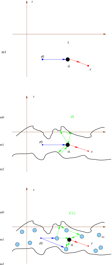
Figure 6: Graphical representation of $\overline{\boldsymbol{t}}^{11}_{\boldsymbol{r}_{i}}$, $\overline{\boldsymbol{t}}^{11}_{S,\boldsymbol{r}_{i}}$,$\overline{\boldsymbol{C}}^{11}_{SV,\boldsymbol{r}_{i}}$

.

The operator $\overline{\boldsymbol{t}}^{11}_{\boldsymbol{r}_{i}}$ describes the scattering process by a particle in an infinite homogenous medium (Figure 6). We must be careful in determining the permittivity of this particle. In fact, as the propagator between two scattering events inside the particle is $\overline{\boldsymbol{G}}_{1}^{\infty}$, the homogeneous medium surrounding the particle has the permittivity $\epsilon_{e}$ due to the definition of $\overline{\boldsymbol{G}}_{1}^{\infty}$ (B). However, $\overline{\boldsymbol{t}}^{11}_{\boldsymbol{r}_{i}}$ doesn’t describe the scattering by a particle of permittivity $\epsilon_{s}$ inside a medium of permittivity $\epsilon_{e}$. If this was correct, the operator $\overline{\boldsymbol{v}}^{11}_{\boldsymbol{r}_{i}}$ defined by (129, 130) would contain the factor $\epsilon_{s}-\epsilon_{e}$ and not the factor $\epsilon_{s}-\epsilon_{1}$. Thus, we have to renormalize the particle permittivity in introducing $\tilde{\epsilon}_{s}=\epsilon_{s}-(\epsilon_{1}-\epsilon_{e})$, such as

$$\overline{\boldsymbol{v}}^{1}_{\boldsymbol{r}_{i}}(\boldsymbol{r}) =K_{vac}^{2}(\epsilon_{s}-\epsilon_{1})\Theta_{s}(\boldsymbol{r}-\boldsymbol{r}_{i})\overline{\boldsymbol{I}}\,,$$ (152)

$$=K_{vac}^{2}(\tilde{\epsilon}_{s}-\epsilon_{e})\Theta_{s}(\boldsymbol{r}-\boldsymbol{r}_{i})\overline{\boldsymbol{I}}\,.$$ (153)

Hence, the operator $\overline{\boldsymbol{t}}^{11}_{\boldsymbol{r}_{i}}$ is the scattering operator for a single particle of permittivity $\tilde{\epsilon}_{s}$ surrounded by an infinite medium of permittivity $\epsilon_{e}$.

The operator $\overline{\boldsymbol{t}}^{11}_{S,\boldsymbol{r}_{i}}$ describes the scattering process by a particle located at $\boldsymbol{r}_{i}$ inside the volume $V_{1}$ of our slab (Figure 6). If we iterate equation (149),

$$\overline{\boldsymbol{t}}^{11}_{S,\boldsymbol{r}_{i}}=\overline{\boldsymbol{t}}^{11}_{\boldsymbol{r}_{i}}+\overline{\boldsymbol{t}}^{11}_{\boldsymbol{r}_{i}}\cdot\delta\overline{\boldsymbol{G}}_{S}^{11}\cdot\overline{\boldsymbol{t}}^{11}_{\boldsymbol{r}_{i}}+\overline{\boldsymbol{t}}^{11}_{\boldsymbol{r}_{i}}\cdot\delta\overline{\boldsymbol{G}}_{S}^{11}\cdot\overline{\boldsymbol{t}}^{11}_{\boldsymbol{r}_{i}}\cdot\delta\overline{\boldsymbol{G}}_{S}^{11}\cdot\overline{\boldsymbol{t}}^{11}_{\boldsymbol{r}_{i}}+\dots\,,$$ (154)

we see that the first term is the scattering process due to the particle, and the following terms describe the interaction between the particle and the boundaries (Figure 6) since the terms $\delta\overline{\boldsymbol{G}}_{S}^{11}$ come from the slab surfaces.

If we now look at equation (143), we see that it describes multiple scattering process by different scatterers inside the slab. In fact, if we had defined the Green function $\overline{\boldsymbol{G}}^{11}_{S}$ without introducing the effective medium $\epsilon_{e}(\omega)$ but in taking the permittivity $\epsilon_{1}$, the operators $\overline{\boldsymbol{W}}^{11}$ and $\overline{\boldsymbol{Q}}^{11}_{SV}$ would have been zero operators (since $\epsilon_{e}(\omega)=\epsilon_{1}(\omega)$ in the definition (134, 136) give null contributions), and the iteration of equation (143) show us the multiple scattering process inside the slab [27, 45]:

$$\overline{\boldsymbol{C}}^{11}_{SV,\boldsymbol{r}_{i}}=\overline{\boldsymbol{t}}^{11}_{S,\boldsymbol{r}_{i}}+\sum_{j=1,\,j\neq i}^{N}\,\overline{\boldsymbol{t}}_{S,\boldsymbol{r}_{i}}^{11}\cdot\overline{\boldsymbol{G}}_{S}^{11}\cdot\overline{\boldsymbol{t}}^{11}_{S,\boldsymbol{r}_{j}}\\ +\sum_{j=1,\,j\neq i}^{N}\,\sum_{k=1,\,k\neq j}^{N}\,\overline{\boldsymbol{t}}_{S,\boldsymbol{r}_{i}}^{11}\cdot\overline{\boldsymbol{G}}_{S}^{11}\cdot\overline{\boldsymbol{t}}^{11}_{S,\boldsymbol{r}_{j}}\cdot\overline{\boldsymbol{G}}_{S}^{11}\cdot\overline{\boldsymbol{t}}^{11}_{S,\boldsymbol{r}_{k}}+\dots\,.\\$$

The operator $\overline{\boldsymbol{C}}^{11}_{SV,\boldsymbol{r}_{i}}$ represents the field scattered by a particle located at $\boldsymbol{r}_{i}$ which takes into account all the interaction effects with the other particles and the boundaries. In introducing the effective medium $\epsilon_{e}(\omega)$ in the definition of $\overline{\boldsymbol{G}}^{11}_{S}$, we see in equation (143) that the multiple scattering contributions are attenuated by the factor $\overline{\boldsymbol{Q}}^{11}_{SV}$.

If we now average equation (135), using the definitions (136, 134) and the (CPA) hypothesis (126), we obtain

$$(2\pi)^{2}\,\delta(\boldsymbol{r}-\boldsymbol{r}_{0})\,\epsilon_{e}\,K_{vac}^{2}\,\overline{\boldsymbol{I}}=(2\pi)^{2}\,\delta(\boldsymbol{r}-\boldsymbol{r}_{0})\,\epsilon_{1}\,K_{vac}^{2}\,\overline{\boldsymbol{I}}+<\widetilde{\boldsymbol{T}}_{SV}^{11}(\boldsymbol{r},\boldsymbol{r}_{0})>_{V}\,,$$ (155)

and since the ensemble average can be decomposed with the conditional probabilities (118) and definition (122), we have

$$<\widetilde{\boldsymbol{T}}_{SV}^{11}>_{V} =\sum_{i=1}^{N}\,<\overline{\boldsymbol{C}}^{11}_{SV,\boldsymbol{r}_{i}}>_{V}\,,$$ (156)

$$=\sum_{i=1}^{N}\,\int_{V_{1}}\rmd^{3}\boldsymbol{r}_{i}\,p(\boldsymbol{r}_{i})\,<\overline{\boldsymbol{C}}^{11}_{SV,\boldsymbol{r}_{i}}>_{V;\boldsymbol{r}_{i}}\,,$$ (157)

$$=n\,\int_{V_{1}}\rmd^{3}\boldsymbol{r}_{i}\,<\overline{\boldsymbol{C}}^{11}_{SV,\boldsymbol{r}_{i}}>_{V;\boldsymbol{r}_{i}}\,,$$ (158)

where we have introduced the particles density $n=N/\mathcal{V}_{1}$. To obtain equation (158), we have used the fact that $<\overline{\boldsymbol{C}}^{11}_{SV;\boldsymbol{r}_{i}}>_{V;\boldsymbol{r}_{i}}=<\overline{\boldsymbol{C}}^{11}_{SV;\boldsymbol{r}_{j}}>_{V;\boldsymbol{r}_{j}}$ for $i\neq j$, since we consider a statistical homogeneous random medium.

In averaging equation (143) with the conditional average $<\dots>_{V;\boldsymbol{r}_{i}}$, and using definitions (119, 124) we obtain:

$$<\overline{\boldsymbol{C}}^{11}_{SV,\boldsymbol{r}_{i}}>_{V;\boldsymbol{r}_{i}}=<\overline{\boldsymbol{t}}^{11}_{S,\boldsymbol{r}_{i}}>_{V;\boldsymbol{r}_{i}}+\sum_{j=1,\,j\neq i}^{N}\int_{V_{1}}\rmd^{3}\boldsymbol{r}_{j}p(\boldsymbol{r}_{j}|\boldsymbol{r}_{i})\,\overline{\boldsymbol{t}}_{S,\boldsymbol{r}_{i}}^{11}\cdot\overline{\boldsymbol{G}}_{S}^{11}\cdot<\overline{\boldsymbol{C}}^{11}_{SV,\boldsymbol{r}_{j}}>_{V;\boldsymbol{r}_{i},\boldsymbol{r}_{j}}\,$$

$$\hbox to0.0pt{\hss${}-{}$}<\overline{\boldsymbol{t}}_{S,\boldsymbol{r}_{i}}^{11}\cdot\overline{\boldsymbol{G}}_{S}^{11}\cdot\overline{\boldsymbol{Q}}^{11}_{SV}>_{V;\boldsymbol{r}_{i}}\,.$$ (159)

Since $\overline{\boldsymbol{t}}_{S;\boldsymbol{r}_{i}}^{11}$ is the scattering operator for one particle located at $\boldsymbol{r}_{i}$, it only depends on the variable $\boldsymbol{r}_{i}$ and not on $\boldsymbol{r}_{j}$ with $j\neq i$, and the average $<\cdots>_{V;\boldsymbol{r}_{i}}$ doesn’t act on $\overline{\boldsymbol{t}}_{S;\boldsymbol{r}_{i}}^{11}$. Furthermore, the averaging of equation (136) is

$$<\overline{\boldsymbol{Q}}^{11}_{SV}>_{V;\boldsymbol{r}_{i}}=\overline{\boldsymbol{W}}^{11}+\overline{\boldsymbol{W}}^{11}\cdot\overline{\boldsymbol{G}}_{S}^{11}\cdot<\overline{\boldsymbol{T}}^{11}_{SV}>_{V;\boldsymbol{r}_{i}}\,.$$ (160)

This equation is simplified by the (CPA) condition $<\overline{\boldsymbol{T}}^{11}_{SV}>_{V}=\overline{\boldsymbol{0}}$, which can also be written under the following form:

$$\int_{V_{1}}\rmd^{3}\boldsymbol{r}_{i}\,p(\boldsymbol{r}_{i})\,<\overline{\boldsymbol{T}}^{11}_{SV}>_{V;\boldsymbol{r}_{i}}=0\,.$$ (161)

As the identity in (161) is valid whatever the volume $V_{1}$ is, we have $<\overline{\boldsymbol{T}}^{11}_{SV}>_{V;\boldsymbol{r}_{i}}=\boldsymbol{0}$. Thus, from equation (160), we have:

$$<\overline{\boldsymbol{Q}}^{11}_{SV}>_{V;\boldsymbol{r}_{i}}=\overline{\boldsymbol{W}}^{11}\,.$$ (162)

From the definition (135,136) and the coherent potential approximation, we deduce that:

$$<\overline{\boldsymbol{Q}}^{11}_{SV}>_{V} =\overline{\boldsymbol{W}}^{11}+\overline{\boldsymbol{W}}^{11}\cdot\overline{\boldsymbol{G}}_{S}^{11}\cdot<\overline{\boldsymbol{T}}^{11}_{SV}>_{V}\,,$$ (163)

$$=\overline{\boldsymbol{W}}^{11}\,.$$ (164)

and

$$<\widetilde{\boldsymbol{T}}_{SV}^{11}>_{V} =<\widetilde{\boldsymbol{T}}_{SV}^{11}>_{V}+<\overline{\boldsymbol{Q}}^{11}_{SV}>_{V}\,,$$ (165)

$$=<\overline{\boldsymbol{Q}}^{11}_{SV}>_{V}\,.$$ (166)

Accordingly, from the results (162, 164, 166) and equation (158) we get for $i\in[1,N]$:

$$<\overline{\boldsymbol{Q}}^{11}_{SV}>_{V;\boldsymbol{r}_{i}} =<\widetilde{\boldsymbol{T}}_{SV}^{11}>_{V}$$ (167)

$$=n\,\int_{V_{1}}\rmd^{3}\boldsymbol{r}_{j}\,<\overline{\boldsymbol{C}}^{11}_{SV,\boldsymbol{r}_{j}}>_{V;\boldsymbol{r}_{j}}\,,$$ (168)

and equation (159) is

$$<\overline{\boldsymbol{C}}^{11}_{SV,\boldsymbol{r}_{i}}>_{V;\boldsymbol{r}_{i}}= \overline{\boldsymbol{t}}^{11}_{S,\boldsymbol{r}_{i}}+n\,\overline{\boldsymbol{t}}_{S,\boldsymbol{r}_{i}}^{11}\cdot\overline{\boldsymbol{G}}_{S}^{11}\cdot\int_{V_{1}}\rmd^{3}\boldsymbol{r}_{j}\left[g(||\boldsymbol{r}_{j}-\boldsymbol{r}_{i}||)\,<\overline{\boldsymbol{C}}^{11}_{SV,\boldsymbol{r}_{j}}>_{V;\boldsymbol{r}_{i},\boldsymbol{r}_{j}}\right.$$ (169)

$$\left.\quad-<\overline{\boldsymbol{C}}^{11}_{SV,\boldsymbol{r}_{j}}>_{V;\boldsymbol{r}_{j}}\right]\,,$$

where we have used the approximation $n\simeq(N-1)/\mathcal{V}_{1}$ which is valid for a large number of particle (${N}\gg 1$). Using the same procedure, we can average equation (143) with the conditional average $<\dots>_{V;\boldsymbol{r}_{i},\boldsymbol{r}_{j}}$ and obtain an equation on $<\overline{\boldsymbol{C}}^{11}_{SV,\boldsymbol{r}_{j}}>_{V;\boldsymbol{r}_{i},\boldsymbol{r}_{j}}$ in a function of $<\overline{\boldsymbol{C}}^{11}_{SV,\boldsymbol{r}_{k}}>_{V;\boldsymbol{r}_{i},\boldsymbol{r}_{j},\boldsymbol{r}_{k}}$ and so on. Hence, a hierarchical system of equations can be generated on the unknown $<\overline{\boldsymbol{C}}^{11}_{SV,\boldsymbol{r}_{i}}>_{V;\boldsymbol{r}_{i}}$, $<\overline{\boldsymbol{C}}^{11}_{SV,\boldsymbol{r}_{j}}>_{V;\boldsymbol{r}_{i},\boldsymbol{r}_{j}}$, $<\overline{\boldsymbol{C}}^{11}_{SV,\boldsymbol{r}_{k}}>_{V;\boldsymbol{r}_{i},\boldsymbol{r}_{j},\boldsymbol{r}_{k}}$,…. We close this system by using the Quasi-Crystalline Approximation (QCA) which states that [16, 17, 32, 33, 46]

$$<\overline{\boldsymbol{C}}^{11}_{SV,\boldsymbol{r}_{j}}>_{V;\boldsymbol{r}_{i},\boldsymbol{r}_{j}}=<\overline{\boldsymbol{C}}^{11}_{SV,\boldsymbol{r}_{j}}>_{V;\boldsymbol{r}_{j}}\,.$$ (170)

As was demonstrated by Lax [46], this approximation is strictly valid when the particles have a fixed position, as in a crystal. The quasi-crystalline approximation is equivalent to neglect of the fluctuation of the effective field, acting on a particle located at $\boldsymbol{r}_{j}$, due to a deviation of a particle located at $\boldsymbol{r}_{i}$ from its average position. Under this approximation, the effective permittivity $\epsilon_{e}(\omega)$ satisfies the following system of equations:

$$(2\pi)^{2}\delta(\boldsymbol{r}-\boldsymbol{r}_{0})\,\epsilon_{e}\,K_{vac}^{2}\,\overline{\boldsymbol{I}}=(2\pi)^{2}\delta(\boldsymbol{r}-\boldsymbol{r}_{0})\,\epsilon_{1}\,K_{vac}^{2}\,\overline{\boldsymbol{I}}+n\,\int_{V_{1}}\rmd^{3}\boldsymbol{r}_{i}\,<\overline{\boldsymbol{C}}^{11}_{SV,\boldsymbol{r}_{i}}(\boldsymbol{r},\boldsymbol{r}_{0})>_{V;\boldsymbol{r}_{i}}\,,$$

(171)

$$<\overline{\boldsymbol{C}}^{11}_{SV,\boldsymbol{r}_{i}}>_{V;\boldsymbol{r}_{i}}=\overline{\boldsymbol{t}}^{11}_{S,\boldsymbol{r}_{i}}+n\,\overline{\boldsymbol{t}}_{S,\boldsymbol{r}_{i}}^{11}\cdot\overline{\boldsymbol{G}}_{S}^{11}\cdot\int_{V_{1}}\rmd^{3}\boldsymbol{r}_{j}[g(||\boldsymbol{r}_{j}-\boldsymbol{r}_{i}||)-1]\,<\overline{\boldsymbol{C}}^{11}_{SV,\boldsymbol{r}_{j}}>_{V;\boldsymbol{r}_{j}}\,.$$

(172)

We can simplify these equations by noticing that the contribution $\delta\overline{\boldsymbol{G}}^{11}_{S}$ due to the boundary in $\overline{\boldsymbol{G}}^{11}_{S}=\overline{\boldsymbol{G}}^{\infty}_{1}+\delta\overline{\boldsymbol{G}}^{11}_{S}$ can be neglected in equations (172) and (149) if the following condition $K^{\prime\prime}_{e}H\gg 1$ with $K_{e}^{\prime\prime}=ImK_{e}$ is satisfied. Usually, we define the extinction length as $l_{e}=1/2K^{\prime\prime}_{e}$ and we see that the previous condition means that the slab thickness must be greater than the extinction length.

For example, if we analyze the contribution $\overline{\boldsymbol{G}}_{S}^{1+\,0-}$ of $\delta\overline{\boldsymbol{G}}^{11}_{S}$, we have

$$\overline{\boldsymbol{G}}_{S}^{1+\,0-}(\boldsymbol{r},\boldsymbol{r}_{0})=\frac{\rmi}{2}\int\!\!\!\int\frac{\rmd^{2}\boldsymbol{p}}{(2\pi)^{2}}\frac{\rmd^{2}\boldsymbol{p}_{0}}{(2\pi)^{2}}\, \rme^{\rmi\,\boldsymbol{p}\cdot\boldsymbol{x}-\rmi\,\boldsymbol{p}_{0}\cdot\boldsymbol{x}_{0}+\rmi\,\alpha_{e}(\boldsymbol{p})\,z+\,\rmi\,\alpha_{0}(\boldsymbol{p}_{0})\,z_{0}}$$

$$\times\overline{\boldsymbol{S}}^{\,1+\,0-}\left(\boldsymbol{p}\right|\left.\boldsymbol{p}_{0}\right)\cdot(\overline{\boldsymbol{I}}-\hat{\boldsymbol{k}}^{0\,-}_{\boldsymbol{p}_{0}}\hat{\boldsymbol{k}}^{0\,-}_{\boldsymbol{p}_{0}})\frac{1}{\alpha_{0}(\boldsymbol{p}_{0})}\,,$$

where

$$\overline{\boldsymbol{S}}^{\,1+\,0-}\left(\boldsymbol{p}\right|\left.\boldsymbol{p}_{0}\right)= \int\!\!\!\int\frac{\rmd^{2}\boldsymbol{p}_{1}}{(2\pi)^{2}}\frac{\rmd^{2}\boldsymbol{p}_{2}}{(2\pi)^{2}}\,\rme^{+\rmi(\alpha_{e}(\boldsymbol{p})+\alpha_{e}(\boldsymbol{p}_{1}))\,H}\,$$

$$\times\overline{\boldsymbol{R}}^{21}(\boldsymbol{p}|\boldsymbol{p}_{1})\cdot\left[\overline{\boldsymbol{I}}_{\perp}^{1-1-}(\boldsymbol{p}_{1}|\boldsymbol{p}_{2})+\overline{\boldsymbol{S}}^{\,1-1-}\left(\boldsymbol{p}_{1}\right|\left.\boldsymbol{p}_{2}\right)\right]\cdot\overline{\boldsymbol{T}}^{10}(\boldsymbol{p}_{2}|\boldsymbol{p}_{0})\,,$$

where we have used the following property:

$$\overline{\boldsymbol{R}}^{H\,21}(\boldsymbol{p}|\boldsymbol{p}_{1})=\rme^{+\rmi(\alpha_{e}(\boldsymbol{p})+\alpha_{e}(\boldsymbol{p}_{1}))\,H}\,\overline{\boldsymbol{R}}^{21}(\boldsymbol{p}|\boldsymbol{p}_{1})$$ (175)

We see that $\overline{\boldsymbol{G}}_{S}^{1+\,0-}$ contains a factor:

$$\rme^{\rmi\,\alpha_{e}(\boldsymbol{p})\,(z+H)+\,\rmi\,\alpha_{0}(\boldsymbol{p}_{0})\,z_{0}}\,,$$ (176)

which is negligible far from the lower boundary if we have $K_{e}^{\prime\prime}H\gg 1$, since

$$\rme^{\rmi\,\alpha_{e}(\boldsymbol{p})\,(z+H)}\sim 0\,.$$ (177)

Similarly, we show that far from the boundaries, the other contributions to $\delta\overline{\boldsymbol{G}}^{11}_{S}$ are negligible compared to $\overline{\boldsymbol{G}}^{\infty}_{1}$. Thus, we replace in equation (172) the term $\overline{\boldsymbol{G}}_{S}^{11}$ by $\overline{\boldsymbol{G}}^{\infty}_{1}$ and the operator $\overline{\boldsymbol{t}}^{11}_{S,\boldsymbol{r}_{i}}$ by $\overline{\boldsymbol{t}}^{11}_{\boldsymbol{r}_{i}}$, and we have

$$<\overline{\boldsymbol{C}}^{11}_{SV,\boldsymbol{r}_{i}}>_{V;\boldsymbol{r}_{i}}=\overline{\boldsymbol{t}}^{11}_{\boldsymbol{r}_{i}}+n\,\overline{\boldsymbol{t}}_{\boldsymbol{r}_{i}}^{11}\cdot\overline{\boldsymbol{G}}_{1}^{\infty}\cdot\int_{V_{1}}\rmd^{3}\boldsymbol{r}_{j}[g(||\boldsymbol{r}_{j}-\boldsymbol{r}_{i}||)-1]\,<\overline{\boldsymbol{C}}^{11}_{SV,\boldsymbol{r}_{j}}>_{V;\boldsymbol{r}_{j}}\,$$ (178)

In doing this, we neglect all the boundary effects in the calculation of the effective permittivity $\epsilon_{e}$, and equations obtained are the same used to calculate the effective permittivity in an infinite random medium [16, 17, 33]. In an infinite medium, we can use the Fourier transform to write the equation (178), which is defined by

$$f(\boldsymbol{k}|\boldsymbol{k}_{0})=\int\rmd^{3}\boldsymbol{r}\,\rmd^{3}\boldsymbol{r}_{0}\,\exp(-\rmi\boldsymbol{k}\cdot\boldsymbol{r}+\rmi\boldsymbol{k}_{0}\cdot\boldsymbol{r}_{0})\,f(\boldsymbol{r},\boldsymbol{r}_{0})\,.$$ (179)

In the Fourier space, the translational invariance of the infinite medium implied the following property of the scattering operators $\overline{\boldsymbol{t}}^{11}_{\boldsymbol{r}_{i}}$ (B):

$$\overline{\boldsymbol{t}}^{11}_{\boldsymbol{r}_{i}}(\boldsymbol{k}|\boldsymbol{k}_{0})=\exp(-\rmi\,(\boldsymbol{k}-\boldsymbol{k}_{0})\cdot\boldsymbol{r}_{i})\,\overline{\boldsymbol{t}}^{11}_{o}(\boldsymbol{k}|\boldsymbol{k}_{0})\,,$$ (180)

where $\overline{\boldsymbol{t}}^{11}_{o}(\boldsymbol{k}|\boldsymbol{k}_{0})=\overline{\boldsymbol{t}}^{11}_{\boldsymbol{r}_{i}=\boldsymbol{0}}(\boldsymbol{k}|\boldsymbol{k}_{0})$ is the scattering operator for a particle located at the origin of the coordinate (see [16, 17, 46]). Using the property of (180) and equation (178), we show that $<\overline{\boldsymbol{C}}^{11}_{SV,\boldsymbol{r}_{i}}(\boldsymbol{k}|\boldsymbol{k}_{0})>_{V;\boldsymbol{r}_{i}}$ verifies also a property similar to (180):

$$<\overline{\boldsymbol{C}}^{11}_{SV,\boldsymbol{r}_{i}}(\boldsymbol{k}|\boldsymbol{k}_{0})>_{V;\boldsymbol{r}_{i}}=\exp(-\rmi\,(\boldsymbol{k}-\boldsymbol{k}_{0})\cdot\boldsymbol{r}_{i})\,\overline{\boldsymbol{C}}^{11}_{o}(\boldsymbol{k}|\boldsymbol{k}_{0})\,,$$ (181)

where we have defined $\overline{\boldsymbol{C}}^{11}_{o}(\boldsymbol{k}|\boldsymbol{k}_{0})=<\overline{\boldsymbol{C}}^{11}_{SV,\boldsymbol{r}_{i}=\boldsymbol{0}}(\boldsymbol{k}|\boldsymbol{k}_{0})>_{V;\boldsymbol{r}_{i}=\boldsymbol{0}}$. By using the properties (180, 181) in equations (178,171), we obtain:

$$\epsilon_{e}\,K_{vac}^{2}\,\overline{\boldsymbol{I}}=\epsilon_{1}\,K_{vac}^{2}\,\overline{\boldsymbol{I}}+n\,\overline{\boldsymbol{C}}^{11}_{o}(\boldsymbol{k}_{0}|\boldsymbol{k}_{0})\,,$$ (182)

$$\overline{\boldsymbol{C}}^{11}_{o}(\boldsymbol{k}|\boldsymbol{k}_{0})=\overline{\boldsymbol{t}}^{11}_{o}(\boldsymbol{k}|\boldsymbol{k}_{0})+n\,\int\frac{\rmd^{3}\boldsymbol{k}_{1}}{(2\pi)^{3}}\,\,h(\boldsymbol{k}-\boldsymbol{k}_{1})\,\overline{\boldsymbol{t}}_{o}^{11}(\boldsymbol{k}|\boldsymbol{k}_{1})\cdot\overline{\boldsymbol{G}}_{1}^{\infty}(\boldsymbol{k}_{1})\cdot\overline{\boldsymbol{C}}^{11}_{o}(\boldsymbol{k}_{1}|\boldsymbol{k}_{0})\,,$$ (183)

where

$$\overline{\boldsymbol{t}}^{11}_{o}=\overline{\boldsymbol{v}}^{11}_{o}+\overline{\boldsymbol{v}}^{11}_{o}\cdot\overline{\boldsymbol{G}}_{1}^{\infty}\cdot\overline{\boldsymbol{t}}^{11}_{o}\,,$$ (184)

$$\overline{\boldsymbol{v}}^{11}_{o}(\boldsymbol{r},\boldsymbol{r}_{0})=\delta(\boldsymbol{r}-\boldsymbol{r}_{0})\,\overline{\boldsymbol{v}}^{11}_{o}(\boldsymbol{r})\,,$$ (185)

$$\overline{\boldsymbol{v}}^{11}_{o}(\boldsymbol{r})=K_{vac}^{2}\,(\tilde{\epsilon}_{s}-\epsilon_{e})\,\Theta_{s}(\boldsymbol{r})\overline{\boldsymbol{I}}$$ (186)

and

$$h(\boldsymbol{k}-\boldsymbol{k}_{1})=\int\rmd^{3}\boldsymbol{r}_{\,}\,\exp(-\rmi\,(\boldsymbol{k}-\boldsymbol{k}_{1})\cdot\boldsymbol{r})\,[g(||\boldsymbol{r}||)-1]\,,$$ (187)

$$\overline{\boldsymbol{G}}_{1}^{\infty}(\boldsymbol{k})=\int\rmd^{3}\boldsymbol{r}\,\exp(-\rmi\boldsymbol{k}\cdot\boldsymbol{r})\,\overline{\boldsymbol{G}}_{1}^{\infty}(\boldsymbol{r})\,.$$ (188)

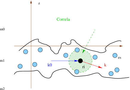
Figure 7: Graphical representation of $<\overline{\boldsymbol{C}}^{11}_{SV,\boldsymbol{r}_{i}}(\boldsymbol{k}|\boldsymbol{k}_{0})>_{V}$

.

In equation (188), we have used the translational invariance of the Green function: $\overline{\boldsymbol{G}}_{1}^{\infty}(\boldsymbol{r},\boldsymbol{r}_{0})=\overline{\boldsymbol{G}}_{1}^{\infty}(\boldsymbol{r}-\boldsymbol{r}_{0})$. Formula (182, 183) is a non-linear system of equations on the unknown $\epsilon_{e}(\omega)$. If we neglect the correlation between the particles (i.e., $h(\boldsymbol{k}-\boldsymbol{k}_{1})=0$) and define the Green function $\overline{\boldsymbol{G}}_{1}^{\infty}$ in replacing the effective permittivity $\epsilon_{e}$ by $\epsilon_{1}$, we obtain the Foldy’s approximation also called the independent scattering approximation (ISA) [27, 47, 26, 16, 17]:

$$\epsilon_{e}\,K_{vac}^{2}\,\overline{\boldsymbol{I}}=\epsilon_{1}\,K_{vac}^{2}\,\overline{\boldsymbol{I}}+n\,\overline{\boldsymbol{t}}^{11}_{o}(\boldsymbol{k}_{0}|\boldsymbol{k}_{0})\Big{|}_{\epsilon_{e}\to\epsilon_{1}}\,.$$ (189)

However, this result is greatly improved under the (CPA-QCA) approach since for Rayleigh scatterers, an approximate formula for $\epsilon_{e}(\omega)$ can be derived from equations (182, 183), which is a generalization of the usual Maxwell-Garnett formula [16, 17, 48, 49, 50]. One can also obtain an approximate formula for the effective permittivity, which at the same time contained the Maxwell-Garnett formula and the Keller approximation [51].

8 Coherent field

By using the expression in (114) and the (CPA) condition (126), the average electric field is

$$<\boldsymbol{E}_{SV}^{0}>_{V}=\boldsymbol{E}^{0i}+\boldsymbol{E}^{0s}_{S}\,.$$ (190)

If we average over the surface disorder, we have

$$\ll\boldsymbol{E}_{SV}^{0}\gg_{SV}=\boldsymbol{E}^{0i}+<\boldsymbol{E}^{0s}_{S}>_{S}\,.$$ (191)

Hence, for an incident plane wave,

$$\boldsymbol{E}^{0i}(\boldsymbol{x},z)=\boldsymbol{E}^{0i}(\boldsymbol{p}_{0})\,\rme^{\rmi\boldsymbol{p}_{0}\cdot\boldsymbol{x}-\rmi\alpha_{0}(\boldsymbol{p}_{0})\,z}\,,$$ (192)

the field in the medium 0 is

$$\ll\boldsymbol{E}_{SV}^{0}(\boldsymbol{x},z)\gg_{SV}=\boldsymbol{E}^{0i}(\boldsymbol{p}_{0})\,\rme^{\rmi\boldsymbol{p}_{0}\cdot\boldsymbol{x}-\rmi\alpha_{0}(\boldsymbol{p}_{0})\,z}\,,$$ (193)

$$+\int\frac{\rmd^{2}\boldsymbol{p}}{(2\pi)^{2}}\,\rme^{\rmi\boldsymbol{p}\cdot\boldsymbol{x}+\rmi\alpha_{0}(\boldsymbol{p})z}\,<\overline{\boldsymbol{S}}^{0+0-}(\boldsymbol{p}|\boldsymbol{p}_{0})>_{S}\cdot\boldsymbol{E}^{0i}(\boldsymbol{p}_{0})\,,$$ (194)

where equations (79, 80, 84) give us

$$\overline{\boldsymbol{S}}^{\,0+\,0-}=\overline{\boldsymbol{R}}^{10}+\overline{\boldsymbol{T}}^{01}\cdot\overline{\boldsymbol{R}}^{H\,21}\cdot[\overline{\boldsymbol{I}}^{1-1-}_{\perp}-\overline{\boldsymbol{R}}^{01}\cdot\overline{\boldsymbol{R}}^{H\,21}]^{-1}\overline{\boldsymbol{T}}^{10}\,.$$ (195)

For statistical homogeneous rough surfaces, we have [21]:

$$<\overline{\boldsymbol{S}}^{0+0-}(\boldsymbol{p}|\boldsymbol{p}_{0})>_{S}=(2\pi)^{2}\,\delta(\boldsymbol{p}-\boldsymbol{p}_{0})\,\overline{\boldsymbol{S}}^{coh}(\boldsymbol{p}_{0})\,,$$ (196)

where $\overline{\boldsymbol{S}}^{coh}(\boldsymbol{p}_{0})$ is a diagonal operator:

$$\overline{\boldsymbol{S}}^{coh}(\boldsymbol{p}_{0})=S^{coh}(\boldsymbol{p}_{0})_{VV}\,\,\hat{\boldsymbol{e}}_{V}^{0+}(\boldsymbol{p}_{0})\hat{\boldsymbol{e}}_{V}^{0-}(\boldsymbol{p}_{0})+S^{coh}(\boldsymbol{p}_{0})_{HH}\,\,\hat{\boldsymbol{e}}_{H}(\boldsymbol{p}_{0})\hat{\boldsymbol{e}}_{H}(\boldsymbol{p}_{0})\,,$$ (197)

or in a matrix form:

$$[\overline{\boldsymbol{S}}^{coh}(\boldsymbol{p}_{0})]=\left(\begin{array}[]{cc}S^{coh}(\boldsymbol{p}_{0})_{VV}&0\\ 0&S^{coh}(\boldsymbol{p}_{0})_{HH}\end{array}\right)\,,$$ (198)

and

$$\ll\boldsymbol{E}_{SV}^{0}(\boldsymbol{x},z)\gg_{SV}=\boldsymbol{E}^{0i}(\boldsymbol{p}_{0})\,\rme^{\rmi\boldsymbol{p}_{0}\cdot\boldsymbol{x}-\rmi\alpha_{0}(\boldsymbol{p}_{0})\,z}+\overline{\boldsymbol{S}}^{coh}(\boldsymbol{p}_{0})\cdot\boldsymbol{E}^{0i}(\boldsymbol{p}_{0})\,\rme^{\rmi\boldsymbol{p}_{0}\cdot\boldsymbol{x}+\rmi\alpha_{0}(\boldsymbol{p}_{0})z}\,.$$

Hence, the coherent field behaves as if the slab was an homogeneous medium of permittivity $\epsilon_{e}$ with planar boundaries but with modified Fresnel coefficients given by the two diagonal elements of $\overline{\boldsymbol{S}}^{coh}_{mat}(\boldsymbol{p}_{0})$.

9 Application

Few approximate theories give explicit expression for the scattering operators (195) for a slab. Most of them use the small-perturbation theory [52, 53, 54, 55, 56, 57] to derive some approximate expression of $\overline{\boldsymbol{S}}^{\,0+\,0-}$, but the perturbative development needs to go up to the second order to take into account the roughness of the surfaces. We must also mention that the Kirchhoff theory in the geometrical optics limit and the full-wave method have been extended for a slab with rough boundaries [58, 59]. However, we know that for the coherent part of the scattered field, the exponential term present in the Kirchhoff theory gives an accurate description even in the small-perturbation limit [60]. Thus, under the Kirchhoff theory (or the first term of Small-Slope Approximation, which gives the same results [21]), we have for Gaussian rough surfaces [21, 16, 17],

$$<\overline{\boldsymbol{R}}^{10}(\boldsymbol{p}|\boldsymbol{p}_{0})>_{S}=(2\pi)^{2}\,\delta(\boldsymbol{p}-\boldsymbol{p}_{0})\,\overline{\boldsymbol{r}}^{10}(\boldsymbol{p}_{0})\rme^{-2\,\alpha_{0}(\boldsymbol{p})^{2}\,\sigma_{1}^{2}}\,,$$ (200)

$$<\overline{\boldsymbol{T}}^{01}(\boldsymbol{p}|\boldsymbol{p}_{0})>_{S}=(2\pi)^{2}\,\delta(\boldsymbol{p}-\boldsymbol{p}_{0})\,\overline{\boldsymbol{t}}^{01}(\boldsymbol{p}_{0})\rme^{-(\alpha_{0}(\boldsymbol{p}_{0})-\alpha_{e}(\boldsymbol{p}_{0}))^{2}\,\sigma_{1}^{2}/2}\,,$$ (201)

$$<\overline{\boldsymbol{R}}^{H\,21}(\boldsymbol{p}|\boldsymbol{p}_{0})>_{S}=(2\pi)^{2}\,\delta(\boldsymbol{p}-\boldsymbol{p}_{0})\,\overline{\boldsymbol{r}}^{H\,21}(\boldsymbol{p}_{0})\rme^{-2\alpha_{e}(\boldsymbol{p}_{0})^{2}\,\sigma_{2}^{2}}\,,$$ (202)

$$<\overline{\boldsymbol{R}}^{01}(\boldsymbol{p}|\boldsymbol{p}_{0})>_{S}=(2\pi)^{2}\,\delta(\boldsymbol{p}-\boldsymbol{p}_{0})\,\overline{\boldsymbol{r}}^{01}(\boldsymbol{p}_{0})\rme^{-2\,\alpha_{e}(\boldsymbol{p}_{0})^{2}\,\sigma_{1}^{2}}\,,$$ (203)

$$<\overline{\boldsymbol{T}}^{10}(\boldsymbol{p}|\boldsymbol{p}_{0})>_{S}=(2\pi)^{2}\,\delta(\boldsymbol{p}-\boldsymbol{p}_{0})\,\overline{\boldsymbol{t}}^{10}(\boldsymbol{p}_{0})\rme^{-(\alpha_{e}(\boldsymbol{p}_{0})-\alpha_{0}(\boldsymbol{p}_{0}))^{2}\,\sigma_{1}^{2}/2}\,,$$ (204)

where $\sigma_{1}$, $\sigma_{2}$ are the rms-heights of the rough surfaces:

$$\sigma_{1}=\sqrt{<h_{1}(\boldsymbol{x})^{2}>_{S}}\,,\qquad\sigma_{2}=\sqrt{<h_{2}(\boldsymbol{x})^{2}>_{S}}\,,$$ (206)

and $\overline{\boldsymbol{r}}^{10}\,,\overline{\boldsymbol{t}}^{01}\,,\overline{\boldsymbol{r}}^{H\,21}\,,\overline{\boldsymbol{r}}^{01}\,,\overline{\boldsymbol{r}}^{01}$ are reflection operators for the planar surface. We write these operators with matrices. For example,

$$\overline{\boldsymbol{r}}^{10}(\boldsymbol{p}_{0})=r^{10}(\boldsymbol{p}_{0})_{VV}\,\,\hat{\boldsymbol{e}}_{V}^{0+}(\boldsymbol{p}_{0})\hat{\boldsymbol{e}}_{V}^{0-}(\boldsymbol{p}_{0})+r^{10}(\boldsymbol{p}_{0})_{HH}\,\,\hat{\boldsymbol{e}}_{H}(\boldsymbol{p}_{0})\hat{\boldsymbol{e}}_{H}(\boldsymbol{p}_{0})$$ (207)

is written

$$[\overline{\boldsymbol{r}}^{10}(\boldsymbol{p}_{0})]=\left(\begin{array}[]{cc}r^{10}(\boldsymbol{p}_{0})_{VV}&0\\ 0&r^{10}(\boldsymbol{p}_{0})_{HH}\end{array}\right)\,,$$ (208)

and we have:

$$[\overline{\boldsymbol{r}}^{10}(\boldsymbol{p}_{0})]=\left(\begin{array}[]{cc}{\textstyle\frac{\epsilon_{e}\alpha_{0}(\boldsymbol{p}_{0})-\epsilon_{0}\alpha_{e}(\boldsymbol{p}_{0})}{\epsilon_{e}\alpha_{0}(\boldsymbol{p}_{0})+\epsilon_{0}\alpha_{e}(\boldsymbol{p}_{0})}}&0\\ 0&{\textstyle\frac{\alpha_{0}(\boldsymbol{p}_{0})-\alpha_{e}(\boldsymbol{p}_{0})}{\alpha_{0}(\boldsymbol{p}_{0})+\alpha_{e}(\boldsymbol{p}_{0})}}\end{array}\right)\,,$$ (211)

$$\left[\overline{\boldsymbol{t}}^{01}(\boldsymbol{p}_{0})\right]=\left(\begin{array}[]{cc}{\textstyle\frac{2\,(\epsilon_{0}\,\epsilon_{e})^{\frac{1}{2}}\,\alpha_{e}(\boldsymbol{p}_{0})}{\epsilon_{e}\alpha_{0}(\boldsymbol{p}_{0})+\epsilon_{0}\alpha_{e}(\boldsymbol{p}_{0})}}&0\\ 0&{\textstyle\frac{2\,\alpha_{e}(\boldsymbol{p}_{0})}{\alpha_{0}(\boldsymbol{p}_{0})+\alpha_{e}(\boldsymbol{p}_{0})}}\end{array}\right)\,,$$ (214)

$$\left[\overline{\boldsymbol{r}}^{H\,21}(\boldsymbol{p}_{0})\right]=\left(\begin{array}[]{cc}{\textstyle\frac{\epsilon_{2}\alpha_{e}(\boldsymbol{p}_{0})-\epsilon_{e}\alpha_{2}(\boldsymbol{p}_{0})}{\epsilon_{2}\alpha_{e}(\boldsymbol{p}_{0})+\epsilon_{e}\alpha_{2}(\boldsymbol{p}_{0})}}&0\\ 0&{\textstyle\frac{\alpha_{e}(\boldsymbol{p}_{0})-\alpha_{2}(\boldsymbol{p}_{0})}{\alpha_{e}(\boldsymbol{p}_{0})+\alpha_{2}(\boldsymbol{p}_{0})}}\end{array}\right)\,\rme^{2\rmi\alpha_{e}(\boldsymbol{p}_{0})H}\,,$$ (217)

$$\left[\overline{\boldsymbol{r}}^{01}(\boldsymbol{p}_{0})\right]=-[\overline{\boldsymbol{r}}^{10}(\boldsymbol{p}_{0})]\,,$$ (218)

$$\left[\overline{\boldsymbol{t}}^{10}(\boldsymbol{p}_{0})\right]=\left(\begin{array}[]{cc}{\textstyle\frac{2\,(\epsilon_{0}\,\epsilon_{e})^{\frac{1}{2}}\,\alpha_{0}(\boldsymbol{p}_{0})}{\epsilon_{e}\alpha_{0}(\boldsymbol{p}_{0})+\epsilon_{0}\alpha_{e}(\boldsymbol{p}_{0})}}&0\\ 0&{\textstyle\frac{2\,\alpha_{0}(\boldsymbol{p}_{0})}{\alpha_{0}(\boldsymbol{p}_{0})+\alpha_{e}(\boldsymbol{p}_{0})}}\end{array}\right)\,.$$ (221)

Hence, in using the independent scattering approximation for the rough surfaces to calculate $<\overline{\boldsymbol{S}}^{\,0+\,0-}>_{S}$,

$$<\overline{\boldsymbol{S}}^{\,0+\,0-}>_{S}=<\overline{\boldsymbol{R}}^{10}>_{S}+<\overline{\boldsymbol{T}}^{01}>_{S}\cdot<\overline{\boldsymbol{R}}^{H\,21}>_{S}\,$$ (222)

$$\cdot[\overline{\boldsymbol{I}}^{1-1-}_{\perp}-<\overline{\boldsymbol{R}}^{01}>_{S}\cdot<\overline{\boldsymbol{R}}^{H\,21}>_{S}]^{-1}\cdot<\overline{\boldsymbol{T}}^{10}>_{S}\,,$$ (223)

we obtain an approximate expression for the diagonal matrix $[\overline{\boldsymbol{S}}^{coh}]$ given by

$$[\overline{\boldsymbol{S}}^{coh}(\boldsymbol{p}_{0})]=[\overline{\boldsymbol{r}}^{10}(\boldsymbol{p}_{0})]\rme^{-2\,\alpha_{0}(\boldsymbol{p}_{0})^{2}\,\sigma_{1}^{2}}+\rme^{-(\alpha_{0}(\boldsymbol{p}_{0})-\alpha_{e}(\boldsymbol{p}_{0}))^{2}\,\sigma_{1}^{2}-2\alpha_{e}(\boldsymbol{p}_{0})^{2}\,\sigma_{2}^{2}}\,[\overline{\boldsymbol{t}}^{01}(\boldsymbol{p}_{0})]\cdot[\overline{\boldsymbol{r}}^{H\,21}(\boldsymbol{p}_{0})]$$

$$\cdot\left([\overline{\boldsymbol{I}}_{2}]-\rme^{-2\,\alpha_{e}(\boldsymbol{p}_{0})^{2}\,(\sigma_{1}^{2}+\sigma_{2}^{2})}\,[\overline{\boldsymbol{r}}^{01}(\boldsymbol{p}_{0})]\cdot[\overline{\boldsymbol{r}}^{H\,21}(\boldsymbol{p}_{0})]\right)^{-1}\cdot[\overline{\boldsymbol{t}}^{10}(\boldsymbol{p}_{0})]\,,$$ (224)

where $[\overline{\boldsymbol{I}}_{2}]=diag(1,1)$ is the two dimensional identity matrix. Using the following identity $[\overline{\boldsymbol{r}}^{10}(\boldsymbol{p}_{0})]^{2}+[\overline{\boldsymbol{t}}^{01}(\boldsymbol{p}_{0})]\cdot[\overline{\boldsymbol{t}}^{10}(\boldsymbol{p}_{0})]=[\overline{\boldsymbol{I}}_{2}]$ ( which is the conservation energy law for a planar surface) and the property in (218), we rewrite equation (224) under the following form:

$$[\overline{\boldsymbol{S}}^{coh}(\boldsymbol{p}_{0})]=\Big{(}[\overline{\boldsymbol{c}}^{1}(\boldsymbol{p}_{0})]\cdot[\overline{\boldsymbol{r}}^{10}(\boldsymbol{p}_{0})]+[\overline{\boldsymbol{c}}^{2}(\boldsymbol{p}_{0})]\,\cdot[\overline{\boldsymbol{r}}^{H\,21}(\boldsymbol{p}_{0})]\Big{)}$$

$$\cdot\Big{(}[\overline{\boldsymbol{I}}_{2}]+[\overline{\boldsymbol{c}}^{3}(\boldsymbol{p}_{0})]\cdot[\overline{\boldsymbol{r}}^{01}(\boldsymbol{p}_{0})]\cdot[\overline{\boldsymbol{r}}^{H\,21}(\boldsymbol{p}_{0})]\Big{)}^{-1}\,,$$ (225)

with

$$[\overline{\boldsymbol{c}}^{1}(\boldsymbol{p}_{0})]=\rme^{-2\,\alpha_{0}(\boldsymbol{p}_{0})^{2}\,\sigma_{1}^{2}}\,[\overline{\boldsymbol{I}}_{2}]\,,$$ (226)

$$[\overline{\boldsymbol{c}}^{2}(\boldsymbol{p}_{0})]=\rme^{-(\alpha_{0}(\boldsymbol{p}_{0})-\alpha_{e}(\boldsymbol{p}_{0}))^{2}\,\sigma_{1}^{2}-2\alpha_{e}(\boldsymbol{p}_{0})^{2}\,\sigma_{2}^{2}}\left([\overline{\boldsymbol{I}}_{2}]-(\rme^{-(\alpha_{0}(\boldsymbol{p}_{0})+\alpha_{e}(\boldsymbol{p}_{0}))^{2}\,\sigma_{1}^{2}}-1)[\overline{\boldsymbol{r}}^{10}(\boldsymbol{p}_{0})]^{2}\right)\,,$$

(227)

$$[\overline{\boldsymbol{c}}^{3}(\boldsymbol{p}_{0})]=\rme^{-2\,\alpha_{e}(\boldsymbol{p}_{0})^{2}\,(\sigma_{1}^{2}+\sigma_{2}^{2})}\,[\overline{\boldsymbol{I}}_{2}]\,.$$ (228)

For a random medium with planar boundaries ($\sigma_{1}=\sigma_{2}=0$), we obtain

$$[\overline{\boldsymbol{S}}^{coh}(\boldsymbol{p}_{0})]=\Big{(}[\overline{\boldsymbol{r}}^{10}(\boldsymbol{p}_{0})]+[\overline{\boldsymbol{r}}^{H\,21}(\boldsymbol{p}_{0})]\Big{)}\cdot\Big{(}[\overline{\boldsymbol{I}}_{2}]+[\overline{\boldsymbol{r}}^{10}(\boldsymbol{p}_{0})]\cdot[\overline{\boldsymbol{r}}^{H\,21}(\boldsymbol{p}_{0})]\Big{)}^{-1}\,,$$ (229)

which is a diagonal matrix which contains the usual reflection coefficients for a planar slab separating three homogeneous medium with the permittivities $\epsilon_{0},\epsilon_{e},\epsilon_{2}$. (See references [16, 17, 52, 53].) In comparing expression (225) and (229), we see that the rough surfaces modify the reflection coefficients for a planar slab by adding new factors $[\overline{\boldsymbol{c}}^{1}]$,$[\overline{\boldsymbol{c}}^{2}]$,$[\overline{\boldsymbol{c}}^{3}]$. The random medium doesn’t change the form of the reflection coefficients but only the permittivity $\epsilon_{1}$ of the initial medium by an effective one $\epsilon_{e}$. Furthermore, if the random medium is highly scattering and thick, the imaginary part of the effective permittivity $\epsilon_{e}$ is important, and the factor $\exp(2\,\rmi\,\alpha_{e}(\boldsymbol{p}_{0})\,H)$ in the expression (217) of $[\overline{\boldsymbol{r}}^{H\,21}]$ is very small. The contribution $[\overline{\boldsymbol{r}}^{H\,21}]$ in equation (229) becomes negligible compared to $[\overline{\boldsymbol{r}}^{10}(\boldsymbol{p}_{0})]$, and we have

$$[\overline{\boldsymbol{S}}^{coh}(\boldsymbol{p}_{0})]=\rme^{-2\,\alpha_{0}(\boldsymbol{p}_{0})^{2}\,\sigma_{1}^{2}}\,[\overline{\boldsymbol{r}}^{10}(\boldsymbol{p}_{0})]\,,$$ (230)

which is the Kirchhoff term for a slab separating two semi-infinite media with the permittivity $\epsilon_{0}$ and $\epsilon_{e}$. In this case, the lower boundary doesn’t contribute to the coherent field.

10 Conclusion

We have considered the scattering of an electromagnetic wave by a random medium with rough boundaries. We have formulated the solution of this problem using two kinds of Green functions. The first one describes the scattering by the rough surfaces and the random medium, and the other represents the scattering by an homogeneous slab with rough boundaries. As equations obtained are similar to those used in scattering theory by an infinite random medium, we were able to introduce the coherent potential with the quasi-crystalline approximation to calculate the effect of the random medium on the coherent field. With this approach, the random medium contribution is taken into account by an effective medium permittivity. The surface scattering contributions on the coherent field are included in the scattering operator of the system, which describes the scattering by the rough boundaries. This operator can be approximated using the usual scattering theories by rough surface like the small-perturbation, the Kirchhoff, or other more sophisticated theories. To derive these results, we have supposed that the slab is sufficiently thick to insure, for one hand, that their exist a layer ($-H+max_{\boldsymbol{x}}h_{2}(\boldsymbol{x})<z<min_{\boldsymbol{x}}h_{1}(\boldsymbol{x})$) between the two rough boundaries which contains the scatterers, and in second hand, that the effective permittivity $\epsilon_{e}(\omega)$ doesn’t not depend on the boundaries ($K_{e}^{\prime\prime}H\gg 1$).

In the following papers, we will use our Green function formulation of the scattering problem to derive a radiative transfer equation describing the scattered incoherent intensity. Furthermore, we will investigate the case of an highly scattering medium where a vectorial diffusion approximation permits simplifying the radiative transfer equation.

Appendix A Green functions

A.1 Scalar Green function

The solution of

$$(\Delta+K_{0}^{2})\,G_{0}(\boldsymbol{r},\boldsymbol{r}_{0})=-\delta(\boldsymbol{r}-\boldsymbol{r}_{0})$$ (231)

in an infinite medium which satisfies the radiation condition at infinity is a generalized function given by

$$G^{\infty}_{0}(\boldsymbol{r}-\boldsymbol{r}_{0})=P.V.\frac{\rme^{\rmi\,K_{0}\,||\boldsymbol{r}-\boldsymbol{r}_{0}||}}{4\pi\,||\boldsymbol{r}-\boldsymbol{r}_{0}||}\,,$$ (232)

where $P.V.$ is the principal value defined by

$$P.V.\int\rmd^{3}\boldsymbol{r}_{0}\,G^{\infty}_{0}(\boldsymbol{r}-\boldsymbol{r}_{0})\,\phi(\boldsymbol{r}_{0})\,=\lim_{a\rightarrow 0}\int_{V-V_{a}(\boldsymbol{r})}\;\;\rmd^{3}\boldsymbol{r}_{0}\,G^{\infty}_{0}(\boldsymbol{r}-\boldsymbol{r}_{0})\,\phi(\boldsymbol{r}_{0})\,,$$ (233)

where $\phi(\boldsymbol{r})$ is a test function, $V_{a}(\boldsymbol{r}_{0})$ is an exclusion volume with size $a$ around the singularity located at $\boldsymbol{r}$. In equation (232), the exclusion volume is a sphere [61]. This generalized function can be represented as the usual spherical function for $\boldsymbol{r}\neq\boldsymbol{r}_{0}$,

$$G^{\infty}_{0}(\boldsymbol{r}-\boldsymbol{r}_{0})=\frac{\rme^{\rmi\,K_{0}\,||\boldsymbol{r}-\boldsymbol{r}_{0}||}}{4\pi\,||\boldsymbol{r}-\boldsymbol{r}_{0}||}\,,,$$ (234)

Using Fourier transform and the residue theorem, we can also write this function under the following form:

$$G^{\infty}_{0}(\boldsymbol{r})=\frac{\rmi}{2}\,\int\frac{\rmd^{2}\boldsymbol{p}}{(2\pi)^{2}}\,\rme^{\rmi\,\boldsymbol{p}\cdot\boldsymbol{x}+\rmi\alpha_{0}(\boldsymbol{p})\,|z|}\frac{1}{\alpha_{0}(\boldsymbol{p})}\qquad\boldsymbol{r}\neq\boldsymbol{0}\,,$$ (235)

The general solution of equation (231) can be expressed with equation (235) as a generalized function:

$$G^{\infty}_{0}(\boldsymbol{r})=P.V.\frac{\rmi}{2}\,\int\frac{\rmd^{2}\boldsymbol{p}}{(2\pi)^{2}}\,\rme^{\rmi\,\boldsymbol{p}\cdot\boldsymbol{x}+\rmi\alpha_{0}(\boldsymbol{p})\,|z|}\frac{1}{\alpha_{0}(\boldsymbol{p})}\qquad\boldsymbol{r}\neq\boldsymbol{0}\,,$$ (236)

where the exclusion volume used in the definition of the principal value (233) is a pillbox of arbitrary cross section but thin in the z direction due to the term $|z|$ in the expression (236) of the Green function [62, 63].

A.2 Dyadic Green function

The solution of

$$\nabla\times\nabla\times\overline{\boldsymbol{G}}_{0}^{\,\infty}(\boldsymbol{r},\boldsymbol{r}_{0})-K_{0}^{2}\,\overline{\boldsymbol{G}}^{\,\infty}_{0}(\boldsymbol{r},\boldsymbol{r}_{0})=\delta(\boldsymbol{r}-\boldsymbol{r}_{0})\,\overline{\boldsymbol{I}}\,$$ (237)

in an infinite medium is a generalized function given by:

$$\overline{\boldsymbol{G}}_{0}^{\,\infty}(\boldsymbol{r}-\boldsymbol{r}_{0})=\left(\overline{\boldsymbol{I}}+\frac{1}{K_{0}^{2}}\nabla\nabla\right)G_{0}^{\infty}(\boldsymbol{r}-\boldsymbol{r}_{0})\,,,$$ (238)

which is short notation for

$$\int\rmd^{3}\boldsymbol{r}_{0}\,\overline{\boldsymbol{G}}_{0}^{\,\infty}(\boldsymbol{r}-\boldsymbol{r}_{0})\,\phi(\boldsymbol{r}_{0})=\left(\overline{\boldsymbol{I}}+\frac{1}{K_{0}^{2}}\nabla\nabla\right)\int\rmd^{3}\boldsymbol{r}_{0}\,G_{0}^{\infty}(\boldsymbol{r}-\boldsymbol{r}_{0})\,\phi(\boldsymbol{r}_{0})\,,$$ (239)

where $\nabla\nabla f(\boldsymbol{r})=\nabla[\nabla f(\boldsymbol{r})]$. When we use the representation (232) or (236) in (238), the action of $\nabla\nabla$ on the exclusion volume $V_{a}(\boldsymbol{r})$ produces a singularity:

$$\overline{\boldsymbol{G}}_{0}^{\,\infty}(\boldsymbol{r}-\boldsymbol{r}_{0})=P.V.\left(\overline{\boldsymbol{I}}+\frac{1}{K_{0}^{2}}\nabla\nabla\right)G_{0}^{\infty}{\boldsymbol{r}-\boldsymbol{r}_{0})}-\frac{1}{K_{0}^{2}}\delta(\boldsymbol{r}-\boldsymbol{r}_{0})\,\overline{\boldsymbol{L}}\,,$$ (240)

where the principal value is defined by

$$P.V.\int\rmd^{3}\boldsymbol{r}_{0}\,\phi(\boldsymbol{r}_{0})\,\left(\overline{\boldsymbol{I}}+\frac{1}{K_{0}^{2}}\nabla\nabla\right)G_{0}^{\infty}(\boldsymbol{r}-\boldsymbol{r}_{0})\,$$

$$=\lim_{a\rightarrow 0}\int_{V-V_{a}(\boldsymbol{r})}\;\;\rmd^{3}\boldsymbol{r}_{0}\,\phi(\boldsymbol{r}_{0})\,\left(\overline{\boldsymbol{I}}+\frac{1}{K_{0}^{2}}\nabla\nabla\right)G_{0}^{\infty}(\boldsymbol{r}-\boldsymbol{r}_{0})\,.$$ (241)

The operator $\overline{\boldsymbol{L}}$ depends on the exclusion volume chosen; for a spherical volume, we have $\overline{\boldsymbol{L}}=\overline{\boldsymbol{I}}/3$, and for a pillbox thin in the z direction, we have $\overline{\boldsymbol{L}}=\hat{\boldsymbol{e}}_{z}\,\hat{\boldsymbol{e}}_{z}$. As $\boldsymbol{r}\neq\boldsymbol{r}_{0}$ in the principal value term, we can use the representation (235) to calculate the first term in (240) and we obtain

$$\overline{\boldsymbol{G}}_{0}^{\,\infty}(\boldsymbol{r},\boldsymbol{r}_{0})=\frac{\rmi}{2}\,P.V.\int\frac{\rmd^{2}\boldsymbol{p}_{0}}{(2\pi)^{2}}\,\rme^{\rmi\,\boldsymbol{p}_{0}\cdot(\boldsymbol{x}-\boldsymbol{x}_{0})+\rmi\,\alpha_{0}(\boldsymbol{p}_{0})\,|z-z_{0}|}\,(\overline{\boldsymbol{I}}-\hat{\boldsymbol{k}}^{0\,\pm}_{\boldsymbol{p}_{0}}\hat{\boldsymbol{k}}^{0\,\pm}_{\boldsymbol{p}_{0}})\,\frac{1}{\alpha_{0}(\boldsymbol{p}_{0})}$$

$$-\frac{1}{K^{2}_{0}}\delta(\boldsymbol{r}-\boldsymbol{r}_{0})\overline{\boldsymbol{L}}\,,$$ (242)

where $\hat{\boldsymbol{k}}^{0\,\pm}_{\boldsymbol{p}_{0}}=\boldsymbol{p}_{0}+sgn(z-z_{0})\,\alpha_{0}(\boldsymbol{p}_{0})\,\hat{\boldsymbol{e}}_{z}$ and

$$sgn(z)=\left\{\begin{array}[]{lc}+1\,,&\mbox{if}\quad z>0\\ 0&\mbox{if}\quad z=0\\ -1&\mbox{if}\quad z<0\end{array}\right.\,.$$ (243)

The upperscript sign in $\hat{\boldsymbol{k}}^{0\,\pm}$ is given by the sign of the function $sgn(z-z_{0})$.

Appendix B Transition operator for one scatterer

The electric field produced by an incident wave $\boldsymbol{E}^{i}(\boldsymbol{r})$ scattered by a spherical particle of radius $r_{s}$, located at $\boldsymbol{r}_{j}$, with a permittivity $\epsilon_{a}$, and surrounded by an infinite medium of permittivity $\epsilon_{b}$ is given by [16, 17, 46]:

$$\boldsymbol{E}(\boldsymbol{r})=\boldsymbol{E}^{i}(\boldsymbol{r})+\int\rmd^{3}\boldsymbol{r}_{1}\,\,\overline{\boldsymbol{G}}^{\infty}_{b}(\boldsymbol{r},\boldsymbol{r}_{1})\cdot\overline{\boldsymbol{v}}^{1}_{\boldsymbol{r}_{j}}(\boldsymbol{r}_{1})\cdot\boldsymbol{E}(\boldsymbol{r}_{1})\,,$$ (244)

where

$$\boldsymbol{v}^{1}_{\boldsymbol{r}_{j}}(\boldsymbol{r}_{1})=K_{vac}^{2}\,(\epsilon_{a}-\epsilon_{b})\,\Theta_{s}(\boldsymbol{r}_{1}-\boldsymbol{r}_{j})\,\overline{\boldsymbol{I}}\,,$$ (245)

and

$$\Theta_{s}(\boldsymbol{r})=\left\{\begin{array}[]{cc}1&\mbox{if}\quad||\boldsymbol{r}||<r_{s}\\ 0&\mbox{if}\quad||\boldsymbol{r}||>r_{s}\end{array}\right.\,.$$ (246)

The Green function $\overline{\boldsymbol{G}}^{\infty}_{b}(\boldsymbol{r},\boldsymbol{r}_{1})$ is defined by

$$\overline{\boldsymbol{G}}_{b}^{\,\infty}(\boldsymbol{r}-\boldsymbol{r}_{0}) =\left(\overline{\boldsymbol{I}}+\frac{1}{K_{b}^{2}}\nabla\nabla\right)G_{b}^{\infty}(\boldsymbol{r}-\boldsymbol{r}_{0})\,,$$ (247)

$$G_{b}^{\infty}(\boldsymbol{r}-\boldsymbol{r}_{0}) =P.V.\frac{\rme^{\rmi\,K_{b}\,||\boldsymbol{r}-\boldsymbol{r}_{0}||}}{4\pi\,||\boldsymbol{r}-\boldsymbol{r}_{0}||}\,,$$ (248)

where $K_{b}^{2}=\epsilon_{b}\,K_{vac}^{2}$. The transition operator for one particle is defined by:

$$\boldsymbol{E}(\boldsymbol{r})=\boldsymbol{E}^{i}(\boldsymbol{r})+\int\rmd^{3}\boldsymbol{r}_{1}\,\rmd^{3}\boldsymbol{r}_{2}\,\,\overline{\boldsymbol{G}}^{\infty}_{b}(\boldsymbol{r},\boldsymbol{r}_{1})\cdot\overline{\boldsymbol{t}}^{11}_{\boldsymbol{r}_{j}}(\boldsymbol{r}_{1},\boldsymbol{r}_{2})\cdot\boldsymbol{E}^{i}(\boldsymbol{r}_{2})\,.$$ (249)

In comparing the definition in (249) with equation (244), we obtain

$$\overline{\boldsymbol{t}}^{11}_{\boldsymbol{r}_{j}}(\boldsymbol{r},\boldsymbol{r}_{0})=\overline{\boldsymbol{v}}^{1}_{\boldsymbol{r}_{j}}(\boldsymbol{r})\,\delta(\boldsymbol{r}-\boldsymbol{r}_{0})+\int\rmd^{3}\boldsymbol{r}_{1}\,\,\overline{\boldsymbol{v}}^{1}_{\boldsymbol{r}_{j}}(\boldsymbol{r})\cdot\overline{\boldsymbol{G}}^{\infty}_{b}(\boldsymbol{r},\boldsymbol{r}_{1})\cdot\overline{\boldsymbol{t}}^{11}_{\boldsymbol{r}_{j}}(\boldsymbol{r}_{1},\boldsymbol{r}_{0})\,.$$ (250)

In the Fourier space, we have

$$\overline{\boldsymbol{t}}^{11}_{\boldsymbol{r}_{j}}(\boldsymbol{k}|\boldsymbol{k}_{0})=\overline{\boldsymbol{v}}^{1}_{\boldsymbol{r}_{j}}(\boldsymbol{k}-\boldsymbol{k}_{0})+\int\frac{\rmd^{3}\boldsymbol{k}_{1}}{(2\pi)^{3}}\,\,\,\overline{\boldsymbol{v}}^{1}_{\boldsymbol{r}_{j}}(\boldsymbol{k}-\boldsymbol{k}_{1})\cdot\overline{\boldsymbol{G}}^{\infty}_{b}(\boldsymbol{k}_{1})\cdot\overline{\boldsymbol{t}}^{11}_{\boldsymbol{r}_{j}}(\boldsymbol{k}_{1}|\boldsymbol{k}_{0})\,,$$ (251)

with

$$\overline{\boldsymbol{v}}^{1}_{\boldsymbol{r}_{j}}(\boldsymbol{k}-\boldsymbol{k}_{0})=\int\rmd^{3}\boldsymbol{r}\,\rme^{-\rmi(\boldsymbol{k}-\boldsymbol{k}_{0})\cdot\boldsymbol{r}}\,\overline{\boldsymbol{v}}^{1}_{\boldsymbol{r}_{j}}(\boldsymbol{r})\,,$$ (252)

and

$$\overline{\boldsymbol{G}}^{\infty}_{b}(\boldsymbol{k}_{1})=\int\rmd^{3}\boldsymbol{r}\,\rme^{-\rmi\boldsymbol{k}_{1}\cdot\boldsymbol{r}}\,\overline{\boldsymbol{G}}^{\infty}_{b}(\boldsymbol{r})\,.$$ (253)

We easily check that $\overline{\boldsymbol{v}}^{1}_{\boldsymbol{r}_{j}}$ verifies the following property:

$$\overline{\boldsymbol{v}}^{1}_{\boldsymbol{r}_{j}}(\boldsymbol{k}-\boldsymbol{k}_{0})=\rme^{-\rmi\,(\boldsymbol{k}-\boldsymbol{k}_{0}).\boldsymbol{r}_{j}}\,\overline{\boldsymbol{v}}^{1}_{o}(\boldsymbol{k}-\boldsymbol{k}_{0})\,,$$ (254)

where $\overline{\boldsymbol{v}}^{1}_{o}(\boldsymbol{k}-\boldsymbol{k}_{0})=\overline{\boldsymbol{v}}^{1}_{\boldsymbol{r}_{j}=\boldsymbol{0}}(\boldsymbol{k}-\boldsymbol{k}_{0})$. In iterating equation (251), and using the property (254), we demonstrate that

$$\overline{\boldsymbol{t}}^{11}_{\boldsymbol{r}_{j}}(\boldsymbol{k}|\boldsymbol{k}_{0})=\exp(-\rmi\,(\boldsymbol{k}-\boldsymbol{k}_{0})\cdot\boldsymbol{r}_{j})\,\overline{\boldsymbol{t}}^{11}_{o}(\boldsymbol{k}|\boldsymbol{k}_{0})\,,$$ (255)

where $\overline{\boldsymbol{t}}^{11}_{o}=\overline{\boldsymbol{t}}^{11}_{\boldsymbol{r}_{j}=\boldsymbol{0}}$ is the transition operator for a particle located at the origin of the coordinate. If we consider an incident plane wave $\boldsymbol{E}^{i}(\boldsymbol{r})$,

$$\boldsymbol{E}^{i}(\boldsymbol{r})=\boldsymbol{E}^{i}(\boldsymbol{k}_{0})\,\rme^{\rmi\boldsymbol{k}_{0}\cdot\boldsymbol{r}}\,,$$ (256)

transverse to the propagation direction $\boldsymbol{k}_{0}$:

$$\hat{\boldsymbol{k}}_{0}\cdot\boldsymbol{E}^{i}(\boldsymbol{k}_{0})=0\quad\Longleftrightarrow\quad(\overline{\boldsymbol{I}}-\hat{\boldsymbol{k}}_{0}\hat{\boldsymbol{k}}_{0})\cdot\boldsymbol{E}^{i}(\boldsymbol{k}_{0})=\boldsymbol{E}^{i}(\boldsymbol{k}_{0})$$ (257)

where $\boldsymbol{k}_{0}=K_{b}\,\hat{\boldsymbol{k}}_{0}$, and $\hat{\boldsymbol{k}}_{0}\cdot\hat{\boldsymbol{k}}_{0}=1$. The far-field scattered by a particle located at the origin is given by

$$K_{b}||\boldsymbol{r}||\gg 1\,,\qquad\boldsymbol{E}(\boldsymbol{r})=\boldsymbol{E}^{i}(\boldsymbol{r})+\frac{\rme^{\rmi\,K_{b}\,||\boldsymbol{r}||}}{4\,\pi\,||\boldsymbol{r}||}\,(\overline{\boldsymbol{I}}-\hat{\boldsymbol{k}}\hat{\boldsymbol{k}})\cdot\overline{\boldsymbol{t}}^{11}_{o}(\boldsymbol{k}|\boldsymbol{k}_{0})\cdot(\overline{\boldsymbol{I}}-\hat{\boldsymbol{k}}_{0}\hat{\boldsymbol{k}}_{0})\cdot\boldsymbol{E}^{i}(\boldsymbol{k}_{0})\,,$$ (258)

where

$$\overline{\boldsymbol{t}}^{11}_{o}(\boldsymbol{k}|\boldsymbol{k}_{0})=\int\rmd^{3}\boldsymbol{r}\,\rmd^{3}\boldsymbol{r}_{0}\,\rme^{-\rmi\boldsymbol{k}\cdot\boldsymbol{r}+\rmi\,\boldsymbol{k}_{0}\cdot\boldsymbol{r}_{0}}\,\overline{\boldsymbol{t}}^{11}_{o}(\boldsymbol{r}|\boldsymbol{r}_{0})\,.$$ (259)

We have used the following far-field approximation to derive the equation (258):

$$\overline{\boldsymbol{G}}_{b}^{\,\infty}(\boldsymbol{r},\boldsymbol{r}_{1})\approx\frac{\rme^{\rmi\,K_{b}\,||\boldsymbol{r}||}}{4\,\pi\,||\boldsymbol{r}||}(\overline{\boldsymbol{I}}-\hat{\boldsymbol{k}}\hat{\boldsymbol{k}})\,\rme^{-\rmi\boldsymbol{k}\cdot\boldsymbol{r}_{1}}\,,$$ (260)

where $\boldsymbol{k}=K_{b}\,\hat{\boldsymbol{r}}$. Usually, the far field scattered by a particle is written in the following form [47, 64, 65]:

$$K_{b}||\boldsymbol{r}||\gg 1\,,\qquad\boldsymbol{E}^{s}(\boldsymbol{r})=\frac{\rme^{\rmi\,K_{b}\,||\boldsymbol{r}||}}{||\boldsymbol{r}||}\,\overline{\boldsymbol{f}}(\hat{\boldsymbol{k}}|\hat{\boldsymbol{k}}_{0})\cdot\boldsymbol{E}^{i}(\boldsymbol{k}_{0})\,.$$ (261)

For spherical scatterer, an exact expression of this operator is well-known and given by the Mie theory [47, 64, 66, 65]. In comparing equations (258) and (261), we have the following relationship between $\overline{\boldsymbol{f}}(\hat{\boldsymbol{k}}|\hat{\boldsymbol{k}}_{0})$ and $\overline{\boldsymbol{t}}^{11}_{o}(\boldsymbol{k}|\boldsymbol{k}_{0})$ :

$$4\pi\,\overline{\boldsymbol{f}}(\hat{\boldsymbol{k}}|\hat{\boldsymbol{k}}_{0})=(\overline{\boldsymbol{I}}-\hat{\boldsymbol{k}}\hat{\boldsymbol{k}})\cdot\overline{\boldsymbol{t}}^{11}_{o}(\boldsymbol{k}|\boldsymbol{k}_{0})\cdot(\overline{\boldsymbol{I}}-\hat{\boldsymbol{k}}_{0}\hat{\boldsymbol{k}}_{0})\,,$$ (262)

where $\boldsymbol{k}=K_{b}\,\hat{\boldsymbol{k}}$, and $\boldsymbol{k}_{0}=K_{b}\,\hat{\boldsymbol{k}}_{0}$. The operator $\overline{\boldsymbol{t}}^{11}_{o}(\boldsymbol{k}|\boldsymbol{k}_{0})$ is a generalization of the scattering amplitude $\overline{\boldsymbol{f}}(\hat{\boldsymbol{k}}|\hat{\boldsymbol{k}}_{0})$ since it contains also the near-field component scattered by the particle. Furthermore, we see that the far-field component is obtained in taking only the transversal components of $\overline{\boldsymbol{t}}^{11}_{o}(\boldsymbol{k}|\boldsymbol{k}_{0})$ (due to the projectors $\overline{\boldsymbol{I}}-\boldsymbol{k}\boldsymbol{k}$ and $\overline{\boldsymbol{I}}-\boldsymbol{k}_{0}\boldsymbol{k}_{0}$) and using an on-shell approximation (since $\boldsymbol{k}\cdot\boldsymbol{k}=\boldsymbol{k}_{0}\cdot\boldsymbol{k}_{0}=K_{b}$).

Appendix C Reciprocity of $\overline{\boldsymbol{C}}^{11}_{o}(\boldsymbol{k}|\boldsymbol{k}_{0})$

In the section 7, we have used the following decomposition of the operator $\overline{\boldsymbol{T}}^{11}_{SV}$:

$$\overline{\boldsymbol{T}}^{11}_{SV}=\overline{\boldsymbol{V}}^{11}+\overline{\boldsymbol{V}}^{11}\cdot\overline{\boldsymbol{G}}_{S}^{11}\cdot\overline{\boldsymbol{T}}^{11}_{SV}\,.$$ (263)

But we could have used this equivalent formulation:

$$\overline{\boldsymbol{T}}^{11}_{SV}=\overline{\boldsymbol{V}}^{11}+\overline{\boldsymbol{T}}_{SV}^{11}\cdot\overline{\boldsymbol{G}}_{S}^{11}\cdot\overline{\boldsymbol{V}}^{11}\,.$$ (264)

According to the section 7, we define a new operator $\widetilde{\boldsymbol{V}}^{11}$ such that:

$$\widetilde{\boldsymbol{V}}^{11}=\overline{\boldsymbol{V}}^{11}+\overline{\boldsymbol{W}}^{11}\,,$$ (265)

where $\overline{\boldsymbol{W}}^{11}$ is defined by equation (134). The operator $\overline{\boldsymbol{T}}^{11}_{SV}$ can also be decomposed in defining new operators $\widetilde{\boldsymbol{T}}^{11}_{SV}$ or $\widetilde{\boldsymbol{TT}}^{11}_{SV}$ and using either equation (263) or (264):

$$\mbox{with the Eq. (\ref{defTg})}\quad\left\{\begin{array}[]{l}\widetilde{\boldsymbol{T}}^{11}_{SV}=\overline{\boldsymbol{T}}^{11}_{SV}+\overline{\boldsymbol{Q}}^{11}_{SV}\,,\\ \overline{\boldsymbol{Q}}^{11}_{SV}=\overline{\boldsymbol{W}}^{11}+\overline{\boldsymbol{W}}^{11}\cdot\overline{\boldsymbol{G}}_{S}^{11}\cdot\overline{\boldsymbol{T}}^{11}_{SV}\,,\end{array}\right.$$ (268)

$$\mbox{with the Eq. (\ref{defTd})}\quad\left\{\begin{array}[]{l}\widetilde{\boldsymbol{TT}}^{11}_{SV}=\overline{\boldsymbol{T}}^{11}_{SV}+\overline{\boldsymbol{QQ}}^{11}_{SV}\,,\\ \overline{\boldsymbol{QQ}}^{11}_{SV}=\overline{\boldsymbol{W}}^{11}+\overline{\boldsymbol{T}}^{11}_{SV}\cdot\overline{\boldsymbol{G}}_{S}^{11}\cdot\overline{\boldsymbol{W}}^{11}\,,\end{array}\right.$$ (271)

Following the demonstration of section 7, we derive the following equations:

$$\left\{\begin{array}[]{l}\widetilde{\boldsymbol{T}}^{11}_{SV}=\sum_{i=1}^{N}\overline{\boldsymbol{C}}^{11}_{SV,\boldsymbol{r}_{i}}\,,\\ \overline{\boldsymbol{C}}^{11}_{SV,\boldsymbol{r}_{i}}=\overline{\boldsymbol{t}}^{11}_{S,\boldsymbol{r}_{i}}+\overline{\boldsymbol{t}}^{11}_{S,\boldsymbol{r}_{i}}\cdot\overline{\boldsymbol{G}}_{S}^{11}\cdot\left(\sum_{j=1,j\neq i}^{N}\overline{\boldsymbol{C}}^{11}_{SV,\boldsymbol{r}_{j}}-\overline{\boldsymbol{Q}}^{11}_{SV}\right)\end{array}\right.$$ (274)

$$\left\{\begin{array}[]{l}\widetilde{\boldsymbol{T}}^{11}_{SV}=\sum_{i=1}^{N}\overline{\boldsymbol{CC}}^{11}_{SV,\boldsymbol{r}_{i}}\,,\\ \overline{\boldsymbol{CC}}^{11}_{SV,\boldsymbol{r}_{i}}=\overline{\boldsymbol{t}}^{11}_{S,\boldsymbol{r}_{i}}+\left(\sum_{j=1,j\neq i}^{N}\overline{\boldsymbol{CC}}^{11}_{SV,\boldsymbol{r}_{j}}-\overline{\boldsymbol{QQ}}^{11}_{SV}\right)\cdot\overline{\boldsymbol{G}}_{S}^{11}\cdot\overline{\boldsymbol{t}}^{11}_{S,\boldsymbol{r}_{i}}\end{array}\right.$$ (277)

If we define the average of the operators $\overline{\boldsymbol{C}}^{11}_{SV,\boldsymbol{r}_{i}}$ and $\overline{\boldsymbol{CC}}^{11}_{SV,\boldsymbol{r}_{i}}$ at the origin ($\boldsymbol{r}_{i}=\boldsymbol{0}$) by:

$$\overline{\boldsymbol{C}}^{11}_{o}=<\overline{\boldsymbol{C}}^{11}_{SV,\boldsymbol{r}_{i}=\boldsymbol{o}}>_{V;\boldsymbol{r}_{i}=\boldsymbol{o}}\,,$$ (278)

$$\overline{\boldsymbol{CC}}^{11}_{o}=<\overline{\boldsymbol{CC}}^{11}_{SV,\boldsymbol{r}_{i}=\boldsymbol{o}}>_{V;\boldsymbol{r}_{i}=\boldsymbol{o}}\,,$$ (279)

we obtain, by using equations (274-277), the following expressions:

$$\overline{\boldsymbol{C}}^{11}_{o}(\boldsymbol{k}|\boldsymbol{k}_{0})=\overline{\boldsymbol{t}}^{11}_{o}(\boldsymbol{k}|\boldsymbol{k}_{0})+n\,\int\frac{\rmd^{3}\boldsymbol{k}_{1}}{(2\pi)^{3}}\,\,h(\boldsymbol{k}-\boldsymbol{k}_{1})\,\overline{\boldsymbol{t}}_{o}^{11}(\boldsymbol{k}|\boldsymbol{k}_{1})\cdot\overline{\boldsymbol{G}}_{1}^{\infty}(\boldsymbol{k}_{1})\cdot\overline{\boldsymbol{C}}^{11}_{o}(\boldsymbol{k}_{1}|\boldsymbol{k}_{0})\,,$$

(281)

$$\overline{\boldsymbol{CC}}^{11}_{o}(\boldsymbol{k}|\boldsymbol{k}_{0})=\overline{\boldsymbol{t}}^{11}_{o}(\boldsymbol{k}|\boldsymbol{k}_{0})+n\,\int\frac{\rmd^{3}\boldsymbol{k}_{1}}{(2\pi)^{3}}\,\,h(\boldsymbol{k}_{1}-\boldsymbol{k}_{0})\,\overline{\boldsymbol{CC}}^{11}_{o}(\boldsymbol{k}|\boldsymbol{k}_{1})\cdot\overline{\boldsymbol{G}}_{1}^{\infty}(\boldsymbol{k}_{1})\cdot\overline{\boldsymbol{t}}_{o}^{11}(\boldsymbol{k}_{1}|\boldsymbol{k}_{0})\,,$$

(282)

Furthermore, under the (CPA) approximation we have $<\overline{\boldsymbol{T}}^{11}_{SV}>_{V}=0$, and from equations (268,271), we deduce that $<\overline{\boldsymbol{Q}}^{11}_{SV}>_{V}=<\overline{\boldsymbol{QQ}}^{11}_{SV}>_{V}=\overline{\boldsymbol{W}}^{11}$ and then

$$<\widetilde{\boldsymbol{T}}^{11}_{SV}>_{V}=<\widetilde{\boldsymbol{TT}}^{11}_{SV}>_{V}\,.$$ (283)

By using the decomposition (274, 277) and the definition of the conditional average $<\,\,>_{V;\boldsymbol{r}_{i}}$, equation (283) can be written as:

$$n\,\int_{V_{1}}\rmd^{3}\boldsymbol{r}_{i}\,<\overline{\boldsymbol{C}}^{11}_{SV,\boldsymbol{r}_{i}}>_{V;\boldsymbol{r}_{i}}=n\,\int_{V_{1}}\rmd^{3}\boldsymbol{r}_{i}\,<\overline{\boldsymbol{CC}}^{11}_{SV,\boldsymbol{r}_{i}}>_{V;\boldsymbol{r}_{i}}\,.$$ (284)

This identity is valid whatever the volume $V_{1}$ and the position $\boldsymbol{r}_{i}$ of the scatterer, and thus we have:

$$\overline{\boldsymbol{C}}^{11}_{o}(\boldsymbol{k}|\boldsymbol{k}_{0})=\overline{\boldsymbol{CC}}^{11}_{o}(\boldsymbol{k}|\boldsymbol{k}_{0})\,.$$ (285)

Hence, the operator $\overline{\boldsymbol{C}}^{11}_{o}(\boldsymbol{k}|\boldsymbol{k}_{0})$ satisfies the following equations:

$$\overline{\boldsymbol{C}}^{11}_{o}(\boldsymbol{k}|\boldsymbol{k}_{0})=\overline{\boldsymbol{t}}^{11}_{o}(\boldsymbol{k}|\boldsymbol{k}_{0})+n\,\int\frac{\rmd^{3}\boldsymbol{k}_{1}}{(2\pi)^{3}}\,\,h(\boldsymbol{k}-\boldsymbol{k}_{1})\,\overline{\boldsymbol{t}}_{o}^{11}(\boldsymbol{k}|\boldsymbol{k}_{1})\cdot\overline{\boldsymbol{G}}_{1}^{\infty}(\boldsymbol{k}_{1})\cdot\overline{\boldsymbol{C}}^{11}_{o}(\boldsymbol{k}_{1}|\boldsymbol{k}_{0})\,,$$

$$\overline{\boldsymbol{C}}^{11}_{o}(\boldsymbol{k}|\boldsymbol{k}_{0})=\overline{\boldsymbol{t}}^{11}_{o}(\boldsymbol{k}|\boldsymbol{k}_{0})+n\,\int\frac{\rmd^{3}\boldsymbol{k}_{1}}{(2\pi)^{3}}\,\,h(\boldsymbol{k}_{1}-\boldsymbol{k}_{0})\,\overline{\boldsymbol{C}}^{11}_{o}(\boldsymbol{k}|\boldsymbol{k}_{1})\cdot\overline{\boldsymbol{G}}_{1}^{\infty}(\boldsymbol{k}_{1})\cdot\overline{\boldsymbol{t}}_{o}^{11}(\boldsymbol{k}_{1}|\boldsymbol{k}_{0})\,.$$

However, since the operator $\overline{\boldsymbol{t}}^{11}_{o}$ is reciprocal and $\overline{\boldsymbol{G}}_{1}^{\infty}(\boldsymbol{k}_{1})=\overline{\boldsymbol{G}}_{1}^{\infty}(-\boldsymbol{k}_{1})$, we easily show using equations (281,282) that $\overline{\boldsymbol{C}}^{11}_{o}(\boldsymbol{k}|\boldsymbol{k}_{0})=[\overline{\boldsymbol{CC}}^{11}_{o}(-\boldsymbol{k}_{0}|-\boldsymbol{k})]^{T}$ where ^T is the transpose of the operator. From the identity (285), we conclude that the operator $\overline{\boldsymbol{C}}^{11}_{o}(\boldsymbol{k}|\boldsymbol{k}_{0})$ is reciprocal:

$$\overline{\boldsymbol{C}}^{11}_{o}(\boldsymbol{k}|\boldsymbol{k}_{0})=[\overline{\boldsymbol{C}}^{11}_{o}(-\boldsymbol{k}_{0}|-\boldsymbol{k})]^{T}\,.$$ (286)

References

References

[1]
Giovannini H, Saillard M and Sentenac A 1998 Numerical study of scattering from
inhomogeneous films
J. Opt. Soc. Am. A15 1182–1191
[2]
Sentenac A, Giovannini H and Saillard M 2002 Scattering from rough
inhomogeneous media : Splitting of surface and volume scattering
J. Opt. Soc. Am. A19 727–736
[3]
Pak K, Tsang L, Li L and Chan C 1993 Combined random rough surface and volume
scattering based on monte-carlo solutions of maxwell’s equation
Radio Science28 331–338
[4]
Lam C M and Ishimaru A 1993 Mueller matrix representation for a slab of random
medium with discrete particles and random rough surfaces with moderate
surface roughness
Waves in Random Media3 111–125
[5]
Lam C M and Ishimaru A 1994 Mueller matrix calculation for a slab of random
medium with both random rough surfaces and discrete particles
IEEE Trans. Ant. Propag.44 145–156
[6]
Ulaby F T, Moore R K and Fung A K 1982 Microwave Remote Sensing vol 3
(Norwood: Artech House)
[7]
Fung A K 1994 Microwave Scattering and Emission Models and Their
Applications (Norwood: Artech House)
[8]
Fung A K and Chen M F 1989 Scattering from a Rayleigh layer with an irregular
interface
Radio Sci.16 1337–1347
[9]
Shin R T and Kong J A 1989 Radiative transfer theory for active remote sensing
of two-layer random medium
Progress In Electromagnetic Research1 359–417
[10]
Mudaliar S 1999 Scattering from a rough layer of a random medium
Waves in Random Media9 521–536
[11]
Mudaliar S 2001 Diffuse waves in a random medium layer with rough boundaries
Waves in Random Media11 45–60
[12]
Mudaliar S 1994 Electromagnetic wave scattering from a random medium layer with
a random interface
Waves in Random Media4 167–176
[13]
Furutsu K 1991 Random-volume scattering: Boundary effects, and enhanced
backscattering
Phys. Rev. A43 2741–2762
[14]
Furutsu K 1983 Random Media and Boundaries - Unified Theory, Two-Scale
Method, and Applications (Berlin: Springer-Verlag)
[15]
Calvo-Perez O 1999
Diffusion des Ondes Électromagétiques par un Film
Diélectrique Rugueux Hétérogènes. Étude Expérimentale
et ModélisationPhD dissertation École Centrale Paris
[16]
Tsang L, Kong J A and Shin R 1985 Theory of Microwave Remote Sensing (New
York: Wiley-Interscience)
[17]
Tsang L and Kong J A 2001 Scattering of Electromagnetics Waves: Advanced
Topics vol 3 (New York: Wiley-Interscience)
[18]
Bass F G and Fuks I M 1979 Wave Scattering from Statistically Rough
Surfaces (Oxford: Pergamon Press)
[19]
Ogilvy J A 1991 Theory of Wave Scattering from Random Rough Surfaces
(Bristol: IOP Publishing)
[20]
Beckmann P and Spizzichino A 1963 The Scattering of Electromagnetic Waves
from Rough Surfaces (Oxford: Pergamon Press)
[21]
Voronovich A G 1994 Wave Scattering from Rough Surfaces (Berlin:
Springer-Verlag)
[22]
Tsang L and Ishimaru A 1987 Radiative wave equations for vector electromagnetic
propagation in dense nontenuous media
J. Electro. Waves. Applic.1 59–72
[23]
Apresyan L A and Kravtsov Y A 1996 Radiation Transfer: Statistical and
Wave Aspects (Amsterdam: Gordon and Breach)
[24]
Kuz’min V L and Romanov V P 1996 Coherent phenomena in light scattering from
disordered systems
Physics Uspekhi39 231–260
[25]
Barabanenkov Y N, Kravtsov Y A, Ozrin V D and Saichev A I 1991 Enhanced
backscattering in optics
Progress in OpticsXXIX 65–197
[26]
Lagendijk A and van Tiggelen B A 1996 Resonnant multiple scattering of light
Physics Reports270 143–216
[27]
Sheng P 1995 Introduction to Wave Scattering, Localization, and Mesoscopic
Phenomena (New York: Academic Press)
[28]
Sheng P (ed) 1990 Scattering and Localization of Classical Waves in Random
Media (Singapore: World Scientific)
[29]
Tai C T 1994 Dyadic Green Functions in Electromagnetic Theory (New York:
IEEE Press)
[30]
Kong J A 1975 Electromagnetic Wave Theory (New York: Wiley-Interscience)
[31]
Soven P 1967 Coherent-potential model of substitutional disordered alloys
Phys. Rev.156 809–813
[32]
Gyorffy B L 1970 Electronic states in liquid metals: A generalization of the
coherent-potential approximation for a system with short-range order
Phys. Rev. B1 3290–3299
[33]
Korringa J and Mills R L 1972 Coherent-potential approximation for random
systems with short-range correlations
Phys. Rev. B5 1654–1655
[34]
Tsang L and Kong J A 1980 Multiple scattering of electromagnetic waves by
random distributions of discrete scatterers with coherent potential and
quantum mechanical formalism
J. Appl. Phys.51 3465–3485
[35]
Tsang L and Ishimaru A 1985 Radiative wave and cyclical transfer equations for
dense nontenuous media
J. Opt. Soc. Am. A2 2187–2194
[36]
Kuga Y, Tsang L and Ishimaru A 1985 Depolarization of the enhanced
retroreflectance from a dense distribution of spherical particles
J. Opt. Soc. Am. A2 616–618
[37]
Rice S O 1951 Reflection of electromagnetic waves from slightly rough surfaces
Comm. Pure Appl. Math.3 351–378
[38]
Voronovich A 1994 Small-slope approximation for electromagnetic wave scattering
at a rough iinterface of two dielectric half-spaces
Waves in Random Media4 337–367
[39]
Bahar E and El-Shenawee M 1994 Vertically and horizontally polarized diffuse
double-scatter cross sections of one-dimensional random rough surfaces that
exhibit enhanced-backscatter-full-wave solutions
J. Opt. Soc. Am. A11 2271–2285
[40]
Álvarez-Pérez J L 2001 An extension of the IEM/IEMM surface
scattering model
Waves in Random Media11 307–329
[41]
DeSanto J A and Brown G 1986
Progress in Optics vol XXIII chapter Multiple Scattering from
Rough Surfaces
North-Holland Amsterdam
[42]
Jackson J D 2001 Classical Electrodynamics (New York: John Wiley & Sons)
[43]
Bennett J M and Mattsson L 1990 Introduction to Surface Roughness and
Scattering (Washington: Optical Society of America)
[44]
Ishimaru A 1978 Wave Propagation and Scattering in Random Media vol 1
(New York: Academic Press)
[45]
Frish U
Wave propagation in random medium
In Bharuch-Reid (ed), Probabilistic Methods in Applied
Mathematics vol 1 Academic Press New York 1968
[46]
Lax M 1952 Multiple scattering of waves. II. the effective field in dense
systems
Phys. Rev.85 621–629
[47]
Ishimaru A 1978 Wave Propagation and Scattering in Random Media vol 2
(New York: Academic Press)
[48]
de Vries P, van Coevorden D V and Lagendijk A 1998 Point scatterers for
classical waves
Rev. Mod. Phys.70 447–466
[49]
Lagendijk A, Nienhuis B, van Tiggelen B A and de Vries P 1997 Microscopic
approach to the lorentz cavity in dielectrics
Phys. Rev. Lett.79 657–660
[50]
Kittel C 1998 Physique de l’État Solide (Paris: Dunod) 7 edition
[51]
Soubret A and Berginc G 2002 Effective dielectric constant for a random medium
Preprint arXiv:physics/0312117
[52]
Fuks I M 2001 Wave diffraction by rough boundary of an arbitrary plane-layered
medium
IEEE Trans. Ant. Propag.49 630–639
[53]
Fuks I M and Voronovich A G 2000 Wave diffraction by rough interfaces in an
arbitrary plane-layered medium
Waves in Random Media10 253–272
[54]
Soubret A, Berginc G and Bourrely C 2001 Application of reduced Rayleigh
equations to electromagnetic wave scattering by two-dimensional randomly
rough surfaces
Phys. Rev. B63 245411–245431
[55]
Soubret A, Berginc G and Bourrely C 2001 Backscattering ehancement of an
electromagnetic wave scattered by two-dimensional rough layers
J. Opt. Soc. Am. A
[56]
Elson J M 1995 Multilayer-coated optics: Guided-wave coupling and scattering by
means of interface random roughness
J. Opt. Soc. Am. A12 729–742
[57]
Bousquet P, Flory F and Roche P 1981 Scattering from multilayer thin films:
Theory and experiment
J. Opt. Soc. Am. A71 1115–1123
[58]
Ohlídal I, Navrátil K and Ohlídal M 1995 Scattering of light from
multilayer systems with rough boundaries
Prog. Opt.34 251–334
[59]
Bahar E and Zhang Y 1999 Diffuse like and cross-polarized fiels scattered from
irregualar layered structures-full-wave analysis
IEEE Trans. Ant. Propag.47 941–948
[60]
Baylard C, Greffet J J and Maradudin A A 1993 Coherent reflection factor of
random rough surface : applications
J. Opt. Soc. Am. A10 2637–2647
[61]
Hanson G W and Yakovlev A B 2002 Operator Theory for Electromagnetics
(New York: Springer)
[62]
van Bladel J 1991 Singular Electromagnetics Fields and Sources (Oxford:
Clarendon Press)
[63]
Yaghjian A D 1980 Electric dyadic green’s functions in the source region
In Proceedings of the IEEE vol 68 248–263
[64]
van de Hulst H C 1957 Light Scattering by Small Particles (New York:
Dover Publications, Inc.)
[65]
Bohren C and Huffman D 1983 Absorption and Scattering of Light by by Small
Particles (New York: Wiley-Interscience)
[66]
Kerker M 1969 The Scattering of Light (New York: Academic Press)