Quasi-geostrophic model of the instabilities of the Stewartson layer

Abstract

We study the destabilization of a shear layer, produced by differential rotation of a rotating axisymmetric container. For small forcing, this produces a shear layer, which has been studied by Stewartson and is almost invariant along the rotation axis. When the forcing increases, instabilities develop. To study the asymptotic regime (very low Ekman number $E$), we develop a quasi-geostrophic two-dimensional model, whose main original feature is to handle the mass conservation correctly, resulting in a divergent two-dimensional flow, and valid for any container provided that the top and bottom have finite slopes. We use it to derive scalings and asymptotic laws by a simple linear theory, extending the previous analyses to large slopes (as in a sphere), for which we find different scaling laws. For a flat container, the critical Rossby number for the onset of instability evolves as $E^{3/4}$ and may be understood as a Kelvin-Helmoltz shear instability. For a sloping container, the instability is a Rossby wave with a critical Rossby number proportional to $\beta E^{1/2}$, where $\beta$ is related to the slope. We also investigate the asymmetry between positive and negative differential rotation and propose corrections for finite Ekman and Rossby numbers. Implemented in a numerical code, our model allows us to study the onset over a broad range of parameters, determining the threshold but also other features such as the spatial structure. We also present a few experimental results, validating our model and showing its limits.

I Introduction

I.1 Background

The destabilization of a shear layer in a rotating system is of general geophysical interest. Shear layers dominated by the Coriolis force, are found in natural systems, as in the atmosphere or in the ocean, as well as on other planets like the jets of Jupiter, which might be unstable and responsible for the observed big eddies.

This work considers the shear layer produced by differential rotation of the boundaries of a fast rotating container, in axisymmetric geometries. The linear problem resulting in cylindrical shear layers aligned with the axis of rotation has been studied by Stewartson (1966) in the spherical shell geometry. He pointed out the nested shear layer structure and their scaling. This problem is closely related to the simpler case of a split cylinder solved earlier by Stewartson (1957) too. In that case, the structure of the shear layer is simpler, but there is still a nested structure. The general structure of these detached shear layers is studied by Moore & Saffman (1969) by focusing on the singularities of the boundary-layer equations. Later, a numerical study has been done by Dormy et al. (1998), recovering the features and scalings predicted by Stewartson.

The linear stability of this kind of layers has been theoretically investigated by Busse (1968) who applied a linear stability theory to the pressure equation in both cases of constant and varying depth. He neglected the bulk viscosity but kept the Ekman friction, recovering some kind of Rayleigh criterion, showing that for the flat case, one should expect a critical Rossby number $\mbox{{Ro}}_{c}\sim E^{3/4}$ (where $E$ is the Ekman number). For a varying depth container, he discussed the criterion obtained by Kuo (1949).

One may notice that the difference between flat and varying depth containers has been made explicit by Busse (1970) for thermal instabilities in rapidly rotating systems : for a flat container the instability is of Bénard type (critical Rayleigh number $Ra_{c}$ independent of Ekman number), whereas for a spherical shell the instability is a thermal Rossby wave ($Ra_{c}\sim E^{-1/3}$).

The setup of Hide & Titman (1967), with a central horizontal disk rotating differentially in a flat cylindrical tank, gives unexpected results which are not yet well understood. They also observed a strong asymmetry between positive and negative differential rotation. Later, Niino & Misawa (1984) performed a similar experiment but with the differential rotation concentrated on the bottom of their flat tank. They find a critical local Reynolds number for the destabilization of the flow, independent of the Ekman number. Their linear theory which includes both Ekman friction and bulk viscosity is in very good agreement with their results. They point out that the bulk viscosity is very important to reproduce accurately the experimental results. They showed that a critical local Reynolds number (defined for the shear layer) describes the threshold of instability properly.

Later, Früh & Read (1999) reproduced almost exactly the case studied by Stewartson (1957). The stability threshold they found is still governed by a critical local Reynolds number, but the theory of Niino & Misawa predicts a value much lower than the observed one. They also observed that the behavior of the flow does not depend strongly on the sign of the differential rotation.

The shear-flow instabilities in a parabolic tank and a free surface was investigated by van de Konijnenberg et al. (1999). They studied both cases with constant depth or varying depth and pointed out that the varying depth has a stabilizing effect, as predicted by the linear theory. However, their setup uses the centrifugal force to adjust the slope of the free surface, so that the slope is directly related to the rotation rate.

More recently, using a 3D code, Hollerbach (2003) studied the differences between positive and negative differential rotation for the onset of these instabilities, pointing out the importance of the geometry of the container.

Hollerbach (2003) computed numerical solutions for the instability of the Stewartson layer between two rotating spheres. Meanwhile, we ran the corresponding experiment, measuring the threshold. Details of the experimental setup can be found in §VI.3.1. The results of theses two studies are in agreement, and summarized in figure 1.

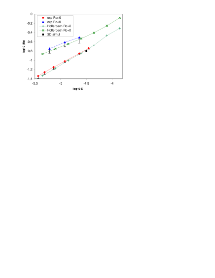
Figure 1: Critical Rossby number versus Ekman number for the spherical shell geometry. The results obtained numerically by Hollerbach (2003) and our lab experiment are in good agreement. The symbols represent established instability, and the error bars the domain where instability was not always clear. ”3D simul” is a run with our own 3D code.

The study of Dormy et al. (1998) showed that the asymptotic regime of the Stewartson problem cannot be illustrated numerically for Ekman numbers higher than $10^{-5}$. Unfortunately, neither the experimental nor the numerical approaches were able to reach Ekman numbers lower than $10^{-5.5}$. This number should be compared with geophysical flows, where Ekman numbers can be much smaller : for the Jovian atmosphere, the oceans and the Earth core the Ekman number is smaller than $10^{-10}$.

I.2 Outline

To study the very low Ekman number regimes we use a quasi-geostrophic (QG) model, detailed in §II : we derive the equations of an improved QG-model, that will be used to address the problem in the next sections, through numerical computations and theoretical analysis of the equations. This QG-model is improved over previous ones by taking into account the mass conservation and Ekman friction. The latter is also dynamically important for non-linear regimes because of its dissipative nature. We were able to benchmark this model with some fully 3D computations by Hollerbach (2003) and the results are quite encouraging.

§III presents results concerning the Stewartson layer, comparing the QG-model with existing results, showing its ability to reproduce the axisymmetric flow. A numerical code based on the quasi-geostrophic approximation allows us to reach Ekman numbers as low as $10^{-10}$ which is very likely to lie in the asymptotic regime, from which extrapolations can be made to even lower Ekman numbers.

In §IV, using numerical calculations as well as theoretical arguments, we investigate the spatial structure of the instability and its asymptotic evolution when lowering the Ekman number. When a $\beta$-effect is present, the instability is a Rossby wave, and consequently we find that its spatial structure changes dramatically with the sign of the differential rotation. This explains the asymmetric sensitivity to geometry studied by Hollerbach (2003). Another interesting feature is that the radial extent of the instability may be independent of the Ekman number in some particular cases.

In §V we derive the scaling laws expected in the asymptotic regime, focusing on the stability threshold. For a flat container, an $E^{3/4}$ law is recovered for the critical Rossby number. We extend this study to finite slopes, in which case the scaling changes to $\beta E^{1/2}$, where $\beta$ is related to the slope. This scaling is the one that should be applied to spherical shells. We perform an analysis leading to a Rayleigh-like criterion, which allows us to evaluate quantitatively the effect of the asymmetry induced by the Rossby wave mechanism. Numerical results obtained with our QG-model are also reported here, for various geometries.

§VI compares our results with previous experiments, as well as with our own, to span a wide range of different geometries. Despite the lack of quantitative agreement between numerical results obtained with the QG-model and the experimental data, the global behaviour of the instability is captured. Finally we conclude in §VII with a discussion.

II Quasi-geostrophic model

The two-dimensional quasi-geostrophic (QG) model we present here has been developed to study the dynamics of a fluid in a rapidly rotating container, invariant by rotation around the rotation axis, without being restricted to the small slope case. We use the cylindrical coordinate system (${\mbox{$e_{r}$}},{\mbox{$e_{\phi}$}},{\mbox{$e_{z}$}}$), with $r$ the distance to the axis, $\phi$ the angle in the plane perpendicular to that axis, and $z$ the height. The container is defined by two functions $z=L_{+}(r)$ and $z=L_{-}(r)$, for the top and the bottom surfaces respectively. Here, we first restrict to the simpler case where $L(r)=L_{+}(r)=-L_{-}(r)$.

In a frame rotating at angular velocity $\Omega_{0}$ around the vertical axis $z$, the flow is described by the Navier-Stokes equation for an incompressible fluid with constant density, including the Coriolis force :

$$\frac{\partial{\mbox{$u$}}}{\partial t}+\left({\mbox{$u$}}.{\mbox{$\nabla$}}\right){\mbox{$u$}}+2{\mbox{$\Omega_{0}$}}\wedge{\mbox{$u$}}=-{\mbox{$\nabla$}}\Pi+\nu\nabla^{2}{\mbox{$u$}}$$ (1)

where $u$ is the fluid velocity field, $\nu$ the kinematic viscosity, and $\Pi$ the reduced pressure field, including centrifugal and gravity potentials. We introduce a velocity scale $U$, a time scale ${\Omega_{0}}^{-1}$ and as typical length scale $R$ the radial size of the container. We then rewrite equation 1 with non-dimensional quantities :

$$\frac{\partial{\mbox{$u$}}}{\partial t}+\mbox{{Ro}}\left({\mbox{$u$}}.{\mbox{$\nabla$}}\right){\mbox{$u$}}+2{\mbox{$e_{z}$}}\wedge{\mbox{$u$}}=-{\mbox{$\nabla$}}\Pi+E\nabla^{2}{\mbox{$u$}}$$ (2)

with $\mbox{{Ro}}\equiv U/R\Omega_{0}$ the Rossby number, $E\equiv\nu/R^{2}\Omega_{0}$ the Ekman number, and $e_{z}$ the unit vector along the rotation axis.

In our study, we take for typical velocity the one based on the differential rotation $U=R\Delta\Omega$, which is supposed to dominate. Hence, the Rossby number reduces to $\Delta\Omega/\Omega_{0}$.

II.1 $z$-averaged vorticity equation

For vanishing Ekman and Rossby number, the Proudman-Taylor theorem ensures that the flow is invariant along the rotation axis direction ($\frac{\partial{\mbox{$u$}}}{\partial z}=0$). This suggests that for small Rossby and Ekman numbers, the $z$-variations should be weak and we expect the flow to be mainly two-dimensional for long-period motions ($\gg\Omega_{0}^{-1}$).

We define the $z$-averaging $\left\langle\;\right\rangle$ by

$$\left\langle u\right\rangle=\frac{1}{2L}\mathchoice{\displaystyle\int_{-L}^{+L}}{\displaystyle\int_{-L}^{+L}}{\int_{-L}^{+L}}{\int_{-L}^{+L}}u(r,z)\>dz$$ (3)

Keeping in mind that $L$ depends on $r$, we have

$$\frac{\partial\left\langle u\right\rangle}{\partial r}=\left\langle\frac{\partial u}{\partial r}\right\rangle+\frac{1}{L}\frac{\partial L}{\partial r}\left(\frac{u(r,+L)+u(r,-L)}{2}-\left\langle u(r,z)\right\rangle\right)$$

Hence, a sufficient condition for the $r$-derivative to commute with $z$-averaging is that $u$ is independent of $z$, that is $u=\left\langle u\right\rangle$.

We now average the $z$-component of the curl of equation 2 with the additional constraint that $u_{r}$ and $u_{\phi}$ are independent of $z$ (so that we can permute $r$-derivation and $z$-averaging). The $z$-component of the vorticity $\omega$ is denoted by $\omega$ and is also $z$-invariant. We obtain

$$\frac{\partial\omega}{\partial t}+\mbox{{Ro}}\left(u_{r}\frac{\partial\omega}{\partial r}+\frac{u_{\phi}}{r}\frac{\partial\omega}{\partial\phi}\right)-(2+\mbox{{Ro}}\>\omega)\left\langle\frac{\partial u_{z}}{\partial z}\right\rangle=E\nabla^{2}\omega$$ (4)

Note that we keep the vortex stretching term $\left\langle\frac{\partial u_{z}}{\partial z}\right\rangle$. All other terms vanish, without any condition on $u_{z}$.

II.2 Mass conservation

The local mass conservation equation for an incompressible fluid,

$$\frac{1}{r}\frac{\partial ru_{r}}{\partial r}+\frac{1}{r}\frac{\partial u_{\phi}}{\partial\phi}+\frac{\partial u_{z}}{\partial z}=0$$ (5)

implies that $\frac{\partial u_{z}}{\partial z}$ is independent of $z$, so that we can now draw a global picture of the flow in the frame of our QG-model.

• $u_{r}$ and $u_{\phi}$ are $z$-invariant

• $u_{z}$ depends linearly on $z$.

II.3 Boundary conditions and Ekman pumping

At the boundaries, Ekman layers will smooth out the vorticity jump. Their thickness is supposed to be small ($E\ll 1$), and we will use the asymptotic expression given by Greenspan (1968), equation 2.6.13 :

$$\left.{\mbox{$u$}}^{1}.{\mbox{$n$}}\right|_{\pm L}=\frac{1}{2}E^{1/2}\,{\mbox{$n$}}.{\mbox{$\nabla$}}\wedge\left(\frac{{\mbox{$n$}}\wedge\left({\mbox{$u$}}-{\mbox{$U_{b}$}}\right)\mp\left({\mbox{$u$}}-{\mbox{$U_{b}$}}\right)}{\sqrt{\left|{\mbox{$n$}}.{\mbox{$e_{z}$}}\right|}}\right)$$ (6)

where $U_{b}$ is the velocity of the boundary. An important point is that expression 6 is valid for time-dependent flows with time scales larger than a few rotation periods. Greenspan used that expression to study the spin-up process in a sphere, which is a time-dependent flow with time scale of order $E^{-1/2}$, and Brito et al. (2004) show experimental data in very good agreement with this linear theory. It is the suitable approximation for our study, as we will find typical period of order $E^{-1/4}$ in section V. This gives us the appropriate boundary conditions for our problem, allowing us to express the vertical velocity. Defining $\beta$

$$\beta\equiv\frac{1}{L}\left.\frac{\partial L}{\partial r}\right|_{z=L}$$ (7)

we have

$$\frac{\partial u_{z}}{\partial z}=E^{1/2}.P(u_{r},u_{\phi},r)+\beta u_{r}$$ (8)

where $P$ is a function depending on the geometry of the container and linear with respect to the jump of $u_{r}$ and $u_{\phi}$ at the boundary and to their first order derivatives. See Appendix A for the explicit expression for a spherical container.

In the case of a constant-depth container, equation 8 reduces to

$$\frac{\partial u_{z}}{\partial z}=-\frac{E^{1/2}}{2L}\left(\omega-\Omega_{b}\right)$$ (9)

where $\Omega_{b}$ is the vorticity at the boundary.

In the case of vanishing Ekman number, the Ekman pumping could be neglected compared to the $\beta$ term (see §C.2). However, the Ekman friction is a dissipative term whereas the $\beta$-term is not, it is thus expected to play an important role for the non-linear dynamics of quasi-geostrophic flows.

The problem is now reduced to the determination of two components of the velocity, $u_{r}$ and $u_{\phi}$, depending only on $r$ and $\phi$. We also need to set a boundary condition on the sides of the container, to be consistent with the modeling of $\left\langle\frac{\partial u_{z}}{\partial z}\right\rangle$, we have to use a no-slip boundary condition $u_{r}=u_{\phi}=0$. At the center ($r=0$) we impose that $u_{r}$ and $u_{\phi}$ remain finite.

II.4 Scalar pseudo-stream function

We introduce a scalar field $\psi$, defined by

$$u_{r}\equiv\frac{1}{r}\frac{\partial\psi}{\partial\phi}$$ (10)

$u_{\phi}$ is now constrained by the three-dimensional mass conservation equation 5, so that for non-axisymmetric flows,

$$u_{\phi} = -\frac{\partial\psi}{\partial r}-\beta\psi$$ (11)

$$\omega = -\nabla^{2}\psi-\beta\left(\frac{\partial\psi}{\partial r}+\frac{\psi}{r}\right)-\frac{d\beta}{dr}\psi$$ (12)

With these equations, we can see that the $\beta$-terms are negligible for $\beta\lambda\ll 1$, where $\lambda$ is a typical radial length scale of the velocity field variations. The model then reduces to the widely used small slope approximation (see e.g. Busse, 1970; Aubert et al., 2003; Kiss, 2003). It will be shown later, that at the stability threshold, the typical length scale is of order $E^{1/4}$, so that asymptotically and at the threshold of instability, the small slope approximation may even be valid in a sphere. However, increasing the forcing, large scale structures will eventually appear, with up to order-one scales, so that we cannot neglect the $\beta$-terms any more in a fully turbulent computation.

Similar approaches have been developed recently. Kiss (2003) proposed a formulation for ocean modeling but without the mass conservation correction. Zavala Sanson & van Heijst (2002) include the effect of weak topography and Ekman friction. The advantage of their formulation is that the Ekman pumping is considered as a source of horizontal divergence. However the simple expression they used for the Ekman boundary condition implicitly assumes nearly flat topography (small $\beta$).

II.5 Axisymmetric flow

For the axisymmetric flow, the scalar function formalism cannot be applied. As it is simpler to work with the velocity field rather than with the vorticity, we project the Navier-Stokes equation 2 on $e_{\phi}$, noting that $\left({\mbox{$e_{z}$}}\wedge{\mbox{$u$}}\right).{\mbox{$e_{\phi}$}}=u_{r}$ and remembering that $\frac{\partial u_{\phi}}{\partial z}=0$. Averaging over $\phi$ to keep only the axisymmetric component, we obtain

$$\frac{\partial\overline{u}_{\phi}}{\partial t}+\mbox{{Ro}}\left(\overline{u_{r}\frac{\partial u_{\phi}}{\partial r}}+\frac{\overline{u_{\phi}u_{r}}}{r}\right)+2\overline{u}_{r}=E\left(\nabla^{2}\overline{u}_{\phi}-\frac{\overline{u}_{\phi}}{r^{2}}\right)$$ (13)

where $\overline{u}$ stands for the $\phi$-average of $u$.

The mass conservation equation reduces to

$$\frac{1}{r}\frac{\partial r\,\overline{u}_{r}}{\partial r}+\frac{\partial\overline{u}_{z}}{\partial z}=0$$

and using equation 8, we can show that $\overline{u}_{r}$ is only due to the Ekman pumping and is directly related to $\overline{u}_{\phi}$ so that the axisymmetric part is actually one-dimensional : $\overline{{\mbox{$u$}}}=\overline{u}_{\phi}(r)\,{\mbox{$e_{\phi}$}}+O(E^{1/2})$. However, non-linear interactions of non-axisymmetric modes can produce axisymmetric flow, so that we keep the terms involving $\overline{u}_{r}$. Furthermore, the Ekman pumping flow $\overline{u}_{r}^{1}$ of order $E^{1/2}$ cannot be neglected. Equation 6 reduces to

$$\overline{u}_{r}^{1}=E^{1/2}\frac{\alpha}{2L}\left(\overline{u}_{\phi}-U_{b}\right)$$ (14)

with

$$\alpha\equiv\left(1+\left(\frac{dL}{dr}\right)^{2}\right)^{1/4}$$ (15)

II.6 Numerical implementation

We wrote a numerical code, that solves the equation of the model described above using the pseudo-stream function formulation. We use a finite difference scheme in the radial direction, and a Fourier expansion in azimuth. The time integration is done using the semi-implicit Cranck Nicholson scheme for the linear part, and a simple Adams-Bashforth scheme for the non-linear terms, which are computed in direct space, as in Aubert et al. (2003).

Our numerical implementation is able to handle various geometries from flat containers to spherical ones.

When compared to fully 3D computations, our QG-model gives quite good results for the basic state flow (see §III) as well as for the stability threshold (see fig. 12 and §VI.2 for more details).

III Stewartson layers

The linear study of shear layers due to differential rotation of the walls has been done in the case of two concentric co-rotating disks (Stewartson, 1957), and in the case of two concentric differentially rotating spheres (Stewartson, 1966).

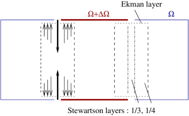
Figure 2: Sketch of the nested Stewartson layers. The arrows show the Ekman pumping inside these layers.

At first order, the flow is invariant along the direction of the rotation axis, and consists of a shear layer which is smoothing out the velocity discontinuity. There are actually two nested layers (see fig. 2) with width scaling like $E^{1/3}$ for the inner layer, and $E^{1/4}$ for the outer one. Note that the $1/3$ layer is not two-dimensional and smoothes out the singularity in the Ekman pumping due to the outer layer. For the spherical shell case, the outer layer width scaling is slightly modified to $E^{2/7}$ for $r<r_{0}$ only. Thus, we can expect that the destabilization of the shear layer in both cases will be closely related.

III.1 QG-model predictions

In the linear and stationary regime, when the Rossby number is small equation 13 reduces to a balance between the Ekman pumping term 14 and the viscous forces in the bulk.

$$2E^{1/2}\frac{\alpha}{2L}\left(\overline{u}_{\phi}-U_{b}\right)=E\left(\nabla^{2}\overline{u}_{\phi}-\frac{\overline{u}_{\phi}}{r^{2}}\right)$$ (16)

which defines the Stewartson layer. Introducing $\Delta$, the width of the Stewartson shear layer we easily recover the scaling obtained by Stewartson.

$$\Delta\sim E^{1/4}$$ (17)

Note that the neglected non-linear terms are small if $\mbox{{Ro}}/\Delta\ll 1$. In §V.1 we will find that $\mbox{{Ro}}\sim E^{a}$ with $a\geq 1/2$, validating this approximation near the threshold.

One of the major issues with the QG-model, is that it cannot model the inner $E^{1/3}$-layer. However, according to the numerical study of Dormy et al. (1998), the $E^{1/3}$-layer has a negligible effect on the velocity profile at Ekman numbers smaller than $E=10^{-6}$.

III.2 Numerical results

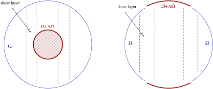
Figure 3: (a) the spherical shell geometry, studied by Stewartson (1966). (b) the split-sphere geometry this paper focuses on.

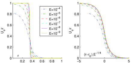
Figure 4: Basic state flow showing the shear layer which scales with $E^{1/4}$ in the asymptotic low Ekman number regime, for $r_{0}=0.35$ in the split-sphere geometry. (a) shows the raw radial profiles and (b) the same profiles rescaled radially, which merge together when $E$ is sufficiently low ($E\leq 10^{-6}$).

The split-sphere geometry consists of a sphere, split at a given cylindrical radius $r_{0}$ (see fig. 3). We solve equation 16 in the frame rotating with the outer part at angular velocity $\Omega_{0}$, while the inner part rotates differentially at $\Delta\Omega$ (positive or negative). This linear problem is solved by a simple matrix inversion using a finite difference radial scheme with variable grid spacing. In this case, the boundary velocity $U_{b}$ is a simple function, $U_{b}=r$ if $r<r_{0}$ and $U_{b}=0$ if $r>r_{0}$. The resulting shear layer for $r_{0}=0.35$ is shown on figure 4. Properly scaled, all these profiles can be superposed in the asymptotic, small Ekman number, regime. The size of the shear layer scales like $E^{1/4}$, as predicted by Stewartson (1957) and the asymptotic regime seems to be attained for $E<10^{-6}$.

The spherical shell (see fig. 3) geometry is the one studied originally by Proudman (1956), and is also of geophysical relevance because the core of the Earth is composed of a solid iron ball ($r_{0}=0.35$) surrounded by liquid iron. The structure of the Stewartson layer in a spherical shell (including the $E^{1/3}$-layer), has been modelled numerically by Dormy et al. (1998), with a fully three dimensional code. We have compared their results with the ones obtained with our QG-model for the spherical shell geometry for $\mbox{{Ro}}=0$ and find that the difference between the two basic state profiles of the angular velocity is always smaller than $0.03$ for $E=10^{-6}$; and for $E=10^{-8}$ the difference never exceeds $0.008$. Hence, we may expect the $E^{1/3}$-layer to play only a minor role at such small Ekman numbers.

IV Spatial structure at the onset

Using our QG-model, we obtained numerically the first unstable mode for four geometries : the flat container; a container with an exponential shape ($\beta=-1$ everywhere); the split-sphere geometry (see fig. 3); and the disk geometry. The latter is a split-sphere where the polar caps have been replaced by flat disks, to mimic our experimental setup (see fig. 13). The first unstable mode is represented on figure 5 for all these geometries.

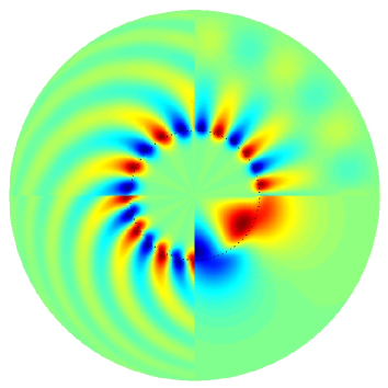
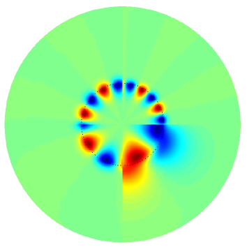
Figure 5: North-pole views of the radial velocity for the first unstable mode at $E=10^{-6}$ for various geometries. Red is positive, blue negative, and green zero. The picture on the left is for $\mbox{{Ro}}>0$, and the one on the right is for $\mbox{{Ro}}<0$. On each picture, (a) shows the constant $\beta=-1$ geometry; (b) shows the split-sphere case; (c) is the disk setup; and (d) is the unstable mode for a flat container ($\beta=0$).

Note that in the reference frame chosen for our computations and for small enough Ekman numbers, the mean flow vanishes in the outer region, whereas the inner region is almost in solid body rotation at the angular velocity $\Delta\Omega=\mbox{{Ro}}\Omega_{0}$ (see figure 4).

IV.1 Dependence on the sign of the Rossby number for $\beta\neq 0$

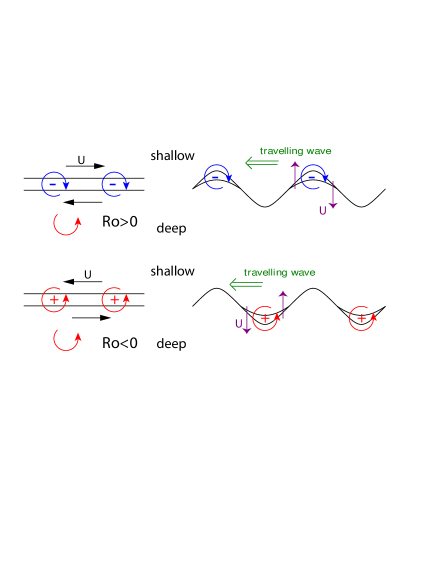
Figure 6: Instability mechanism showing a different spatial behavior depending on the sign of the Rossby number

We can observe on figure 5 that many features depend on the sign of the Rossby number, for $\beta\neq 0$. The most striking one is the spatial behaviour of the split-sphere arrangement (fig. 5b) : for $\mbox{{Ro}}>0$ the instability fills the outer region ($r>r_{0}$) with spiralling arms, whereas for $\mbox{{Ro}}<0$ the critical mode seems to extend more in the inner region ($r<r_{0}$), leaving the outer region almost at rest. The constant $\beta$ case (fig. 5a) also shows long range extension in the outer region for $\mbox{{Ro}}>0$, but no spiralling.

To understand all these features, we must turn to the instability mechanism, which is strongly dominated by the slope $\beta$. Figure 6 sketches this mechanism. For a column of local vorticity $\omega$ moved to a deeper region, the conservation of mass and total vorticity ($2\Omega_{0}+\omega>0$) leads to the following behaviour : If $\omega>0$ the local vorticity is amplified, and if $\omega<0$ it is damped.

Hence, for $\mbox{{Ro}}>0$ the vorticity sheet is negative implying that the perturbation is damped in the deeper region, whereas it is amplified in the shallow region. For $\mbox{{Ro}}<0$, it is the opposite. In both cases, the amplified vorticity will induce a flow which induces a drift of the pattern in the prograde direction (as for any Rossby wave).

This fundamental asymmetry between positive and negative Rossby numbers partly explains the results obtained by Hollerbach (2003). We will discuss an example in §VI.2.

IV.2 Radial scalings

In figure 5abc the perturbation of the shear layer spreads across the whole volume whereas in the flat container case (fig. 5d) or the thermal convection instability in a sphere (see Dormy et al., 2003), it is radially localized. This is explained by a simple model detailed in appendix B, and the main results obtained are summarized in the following lines.

For small $\beta$ as in the inner part of the split-sphere arrangement, the critical mode has a radial extension comparable to its azimuthal scale, without oscillations; but for large $\beta$ as it is the case for the outer part of the split-sphere arrangement, the instability consists of a rapid oscillation of radial length scale $\lambda$ related to the azimuthal wave-number $m$ by

$$\lambda\sim m\sqrt{\left|2\beta\right|}$$ (18)

This rapid oscillation is contained in an envelope of radial size

$$\Lambda\sim\left(2\left|\beta\right|\right)^{-1/2}\alpha^{-1}E^{0}$$ (19)

Equation 19 implies that the radial extent of the perturbation is independent of $E$. This spatial structure corresponds to the spiralling of the Rossby wave observed for variable $\beta$ (see fig. 5bc). We may also notice a fundamental difference with the thermal convection case investigated by Yano (1992) and Jones et al. (2000) where the $E^{1/6}$ radial extension decreases with $E$, so that the instability remains localized for small enough $E$.

IV.2.1 Numerical results

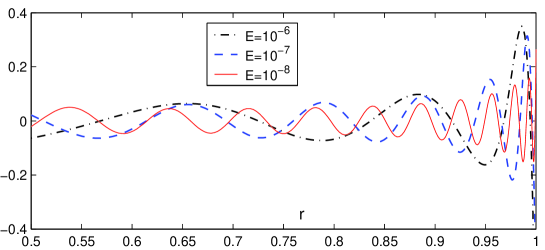
Figure 7: Vorticity profile at fixed $\phi$ at the stability threshold for $\mbox{{Ro}}>0$ in the outer region.

We show in figure 7 a radial vorticity profile (at a fixed $\phi$) obtained with the split-sphere setup. It shows that the vorticity gets amplified by the decreasing depth as approaching the equator, while the spatial frequency of the oscillations increases, in agreement with equation 18. In addition even when decreasing $E$, the perturbation seems to spread across the whole width of the tank, as predicted by the scaling 19. This is not due to the singularity of the QG-model at the equator, because we also observed the same phenomena with a truncated sphere, where the slope remains finite (see §V.3.1).

The scaling 18 is observed quantitatively in numerical simulations as shown on figure 8. On this curves we can also see the effect of the equatorial boundary, which modifies the scaling near $r=1$. When $\beta$ is constant, there is no spiralling but the instability still fills the whole gap, as figure 5a shows.

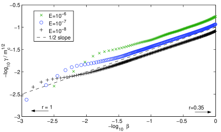
Figure 8: Evolution of the radial size (evaluated using spatial derivation) of the unstable mode near the equatorial singularity for the split-sphere geometry. All these curves exhibit a wide range of slope $1/2$, which is the expected trend to cancel phase-mixing. Near the equatorial boundary ($r=1$) this scaling is no longer valid.

V Asymptotic laws for the onset

V.1 Scaling analysis

We perform a linear stability analysis on equation 4. Let $U(r)\,{\mbox{$e_{\phi}$}}$ be the basic state velocity profile solution of the linear equation 16 (for $\mbox{{Ro}}=0$), and $u$ the perturbation. With $\Omega$ the vorticity associated with $U(r)$ :

$$\Omega=\frac{\partial U}{\partial r}+\frac{U}{r}$$

we find

$$\frac{\partial\omega}{\partial t}+\mbox{{Ro}}\left(u_{r}\frac{\partial\Omega}{\partial r}+\frac{U}{r}\frac{\partial\omega}{\partial\phi}\right)-2\left\langle\frac{\partial u_{z}}{\partial z}\right\rangle=E\nabla^{2}\omega$$ (20)

where we have neglected the small local vorticity $\mbox{{Ro}}\>\Omega$. We now introduce the frequency $f$ of the disturbance, and its azimuthal wave-number $m$.

At the stability threshold, we expect the inertial terms to be both of the same magnitude,

$$\Delta^{-2}\sim m^{2}$$

which implies the wave-number of the perturbation to be comparable to the thickness of the shear layer

$$m\sim\Delta^{-1}\sim E^{-1/4}$$

V.1.1 Without slope

When there is no slope equation 8 reduces to

$$\left\langle\frac{\partial u_{z}}{\partial z}\right\rangle=-\frac{E^{1/2}}{2L}\>\omega$$ (21)

so that equation 20 gives in terms of order of magnitude :

$$mf+\mbox{{Ro}}\>\Delta^{-2}+\mbox{{Ro}}\>m^{2}\sim\frac{E^{1/2}}{L}m+Em^{3}$$

With $m\sim E^{-1/4}$, the stability threshold is given by a balance between the non-linear forcing and the viscous damping :

$$\mbox{{Ro}}_{c}\sim E^{3/4}$$

which is the result obtained by the linear theory of Busse (1968) and by the critical local Reynolds number ($Re\sim\mbox{{Ro}}E^{-3/4}$) theory of Niino & Misawa (1984). It is also consistent with the experimental results of Niino & Misawa (1984) and Früh & Read (1999) and corresponds to a Kelvin-Helmoltz instability of the shear layer.

For an oscillatory instability, the frequency $f$ should be consistent with $mf\sim\mbox{{Ro}}\>m^{2}$, and so

$$f\sim E^{1/2}$$

This effect, if present, may be very difficult to separate from the advection of the pattern, because they are of similar amplitudes.

V.1.2 With slope

When the slope is important, $\frac{\partial u_{z}}{\partial z}\simeq\beta u_{r}$, and so equation 20 gives the following balance :

$$mf+\mbox{{Ro}}\>\Delta^{-2}+\mbox{{Ro}}\>m^{2}+2\beta\sim Em^{3}$$

If again $m\sim E^{-1/4}$, the viscosity is negligible and the stabilization is due to the slope : the instability has to overcome the Proudman-Taylor constraint. As a matter of fact, from a balance between slope and forcing, we find

$$\mbox{{Ro}}_{c}\sim 2\beta E^{1/2}$$ (22)

This is the expected scaling for non-flat containers such as spherical shells, and is quite different from the flat case. This result agrees with the criterion obtained by Kuo (1949) applied to a Stewartson layer.

For a time-dependent instability, the frequency $f$ verifies $mf\sim 2\beta$, and

$$f\sim\frac{2\beta}{m}$$

which is the Rossby wave dispersion relation. At the onset, we may notice that the Ekman pumping is comparable to viscous dissipation in the bulk of the fluid.

V.2 Rossby wave asymmetry effect

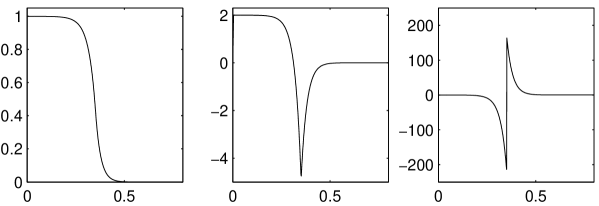
Figure 9: Basic state axisymmetric flow profiles (solution of eq. 16), as a function of radius $r$ for $E=10^{-6}$ and a split-sphere geometry with $r_{0}=0.35$. (a) rotation velocity $U/r$; (b) vorticity $\Omega$; (c) radial derivative of vorticity $\frac{\partial\Omega}{\partial r}$.

As stated in §IV.1, the instability develops as a Rossby wave. Here we give a Rayleigh-like criterion for the onset of instability and use it to evaluate the asymmetry induced by the Rossby wave.

The basic state flow $U$, represented on figure 9 is the solution of the linear equation 16. The sign and amplitude of the forcing are both controlled by the parameter Ro in equation 20. We are looking for solutions of the form $\psi(r,\phi,t)=e^{im\phi+\lambda t}\psi(r)$. We use the $\psi$ formulation introduced in section II.4, but without the $\beta$-terms to keep simpler expressions. Ignoring Ekman friction and viscosity, we obtain from equation 20

$$\left(\lambda+\frac{im}{r}\mbox{{Ro}}U\right)\omega\left[\psi\right]=\left(2\beta-\mbox{{Ro}}\frac{\partial\Omega}{\partial r}\right)\frac{im}{r}\psi$$ (23)

Multiplying by $\psi^{*}L(r)r$ and integrating over $r$ we have

$$\mathchoice{\displaystyle\int_{0}^{1}}{\displaystyle\int_{0}^{1}}{\int_{0}^{1}}{\int_{0}^{1}}\omega\left[\psi\right]\psi^{*}Lr\>dr=\mathchoice{\displaystyle\int_{0}^{1}}{\displaystyle\int_{0}^{1}}{\int_{0}^{1}}{\int_{0}^{1}}\frac{2\beta-\mbox{{Ro}}\frac{\partial\Omega}{\partial r}}{\lambda+\frac{im}{r}\mbox{{Ro}}U}\>im\left|\psi\right|^{2}L\>dr$$ (24)

Expanding the left hand side of this equation, and integrating by part, we obtain

$$\mathchoice{\displaystyle\int_{0}^{1}}{\displaystyle\int_{0}^{1}}{\int_{0}^{1}}{\int_{0}^{1}}\psi^{*}\left(\frac{m^{2}}{r^{2}}\psi-\frac{1}{r}\frac{\partial}{\partial r}\left(r\frac{\partial\psi}{\partial r}\right)\right)Lr\>dr=\mathchoice{\displaystyle\int_{0}^{1}}{\displaystyle\int_{0}^{1}}{\int_{0}^{1}}{\int_{0}^{1}}\frac{m^{2}}{r^{2}}\psi\psi^{*}Lr\>dr+\left[\psi^{*}\frac{\partial\psi}{\partial r}\right]_{0}^{1}-\mathchoice{\displaystyle\int_{0}^{1}}{\displaystyle\int_{0}^{1}}{\int_{0}^{1}}{\int_{0}^{1}}\left|\frac{\partial\psi}{\partial r}\right|^{2}Lr\>dr$$

and from the boundary conditions the bracketed term vanishes, leading to

$$\mathchoice{\displaystyle\int_{0}^{1}}{\displaystyle\int_{0}^{1}}{\int_{0}^{1}}{\int_{0}^{1}}\left(\frac{m^{2}}{r^{2}}\left|\psi\right|^{2}+\left|\frac{\partial\psi}{\partial r}\right|^{2}\right)Lr\>dr=\mathchoice{\displaystyle\int_{0}^{1}}{\displaystyle\int_{0}^{1}}{\int_{0}^{1}}{\int_{0}^{1}}\frac{im\left|\psi\right|^{2}\left(2\beta-\mbox{{Ro}}\frac{\partial\Omega}{\partial r}\right)\left(\lambda^{*}-\frac{im}{r}\mbox{{Ro}}U\right)}{\left|\lambda+\frac{im}{r}\mbox{{Ro}}U\right|^{2}}\>L\>dr$$

With $\Re(\lambda)$ the real part of the complex number $\lambda$, the imaginary part of this equation gives

$$0=\Re(\lambda^{*})\mathchoice{\displaystyle\int_{0}^{1}}{\displaystyle\int_{0}^{1}}{\int_{0}^{1}}{\int_{0}^{1}}\frac{\left|\psi\right|^{2}\left(2\beta-\mbox{{Ro}}\frac{\partial\Omega}{\partial r}\right)}{\left|\lambda+\frac{im}{r}\mbox{{Ro}}U\right|^{2}}\>L\>dr$$ (25)

For a mode to be unstable, we need $\Re(\lambda^{*})\neq 0$, which means that there is an $r$ for which

$$2\beta-\mbox{{Ro}}\frac{\partial\Omega}{\partial r}=0$$ (26)

This is exactly the criterion already obtained by Kuo (1949). Using the complete pseudo-stream function given in section II.4 would lead to the same result. Therefore, the determination of the stability threshold will not be affected by using the small slope approximation, as it is usually done for the thermal convection case (see Busse, 1970).

The critical Rossby number $\mbox{{Ro}}_{c}$ that will satisfy 26 will be obtained for the maximum value $M$ of $\left|\frac{\partial\Omega}{\partial r}\right|$. We must now take care of what value of $\beta$ comes into that expression. Actually, the shear layer samples the values of $\beta$ about $\Delta$ to the left or to the right of the split radius $r_{0}$, depending on the sign of Ro. Then we have

$$\left|\mbox{{Ro}}_{c}^{\pm}\right|=\frac{2\left|\beta(r_{0}\pm\Delta)\right|}{M}$$ (27)

At that point, remembering that the $E^{1/3}$-layer smoothes out discontinuities in $\frac{\partial\Omega}{\partial r}$, we can expect that it will reduce the value of $M$, resulting in an higher $\mbox{{Ro}}_{c}$. Hence, the effect of the $E^{1/3}$-layer may be essentially to increase the critical Rossby number.

Assuming $\beta$ is a smooth function and $\Delta$ is small enough to use a Taylor expansion

$$\left|\beta(r_{0}\pm\Delta)\right|=\left|\beta_{0}\right|\pm\Delta\left(\frac{\partial\left|\beta\right|}{\partial r}\right)_{0}$$

we obtain

$$\left|\mbox{{Ro}}^{\pm}\right|=2\,\Delta^{2}\left(\left|\beta_{0}\right|\pm\Delta\left(\frac{\partial\left|\beta\right|}{\partial r}\right)_{0}\right)$$

This shows a fundamental asymmetry between positive and negative Ro due to the Rossby-wave nature of the instability.

V.3 Numerical results

V.3.1 Split-sphere geometry

In the split-sphere geometry, the slope parameter $\beta$ becomes very large near the equator and the expression of the Ekman pumping we use is no longer valid near the equator as the Ekman layer becomes singular (Roberts & Stewartson (1963); see also §A.3). However, this area is very small and so we expect that it will not affect the determination of the stability threshold. To test this we followed the idea of Yano et al. (2003) and truncated our container at $r=0.9$ to prevent the slope from growing to large near the equator. The solutions showed the same features as the untruncated calculation and very similar stability thresholds.

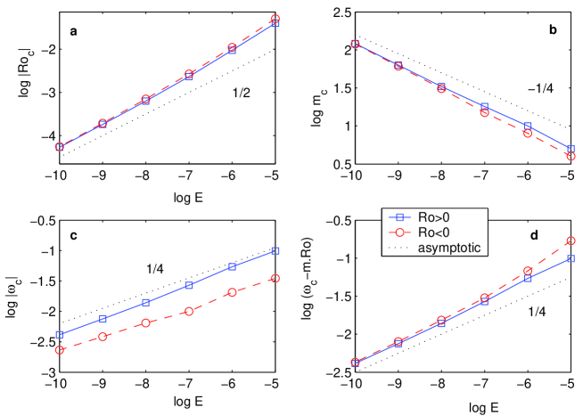
Figure 10: Stability threshold data (given in table C.1) as a function of the Ekman number. (a) represents the threshold; (b) shows the critical wave number; (c) is the raw pulsation at the threshold; (d) is the pulsation corrected for advection effects. Dotted lines indicate the asymptotic exponent obtained in §V.1.2.

The results for the stability threshold are given in appendix C.1 and plotted in figure 10. They seem to match the asymptotical scaling obtained previously, especially for small Ekman numbers. We expect the perturbation to be a Rossby wave and in order to compare its pulsation with the asymptotic laws, we need to correct for the advection by the mean flow. Considering that the outer region (where the $\mbox{{Ro}}>0$ instability develops) is not advected, we don’t correct the $\mbox{{Ro}}>0$ data. However the inner region (where the $\mbox{{Ro}}<0$ case develops) can be considered as in solid body rotation (for small Ekman numbers) and the simplest way to correct for the advection is then to subtract the rotation rate $\Delta\Omega$ from the phase speed $c=\omega/m$ for $\mbox{{Ro}}<0$. The pulsations of the Rossby waves are plotted in figure 10d, and they agree quite well with the asymptotic law, for both positive and negative Ro.

We checked that the difference between critical positive and negative Rossby number is proportional to $E^{1/4}$, in agreement with the findings of §V.2.

With our numerical code, we are able to test various boundary conditions. We report that the boundary conditions (free-slip or no-slip) hardly affect the stability threshold, whereas the presence of Ekman friction has a small yet visible effect. The divergence correction we introduced in §II.4 seems to be negligible at the threshold. The results of these tests are summarized in table C.2.

V.3.2 Other geometries

We report the results of the numerical computations for the four studied geometries. To compare the flat and non-flat case, we set up different geometries and do all the computation using our numerical implementation of the QG-model described in §II. For the flat geometry we choose a flat cylindrical container with a height equal to its diameter. We also set up a container with an exponential shape, defined by $\beta=-1$ everywhere. The split-sphere geometry studied in detail in §V.3.1 and finally the disk setup. This latter geometry is a split-sphere where the polar caps have been replaced by flat disks to mimic our experimental setup (see fig. 13). However, with the QG-model we are not able to take the height-jump at the edge of the disks into account, so the resulting disk geometry is in fact flat for $r<r_{0}$ and spherical for $r>r_{0}$, with no height jump. The results obtained are summarized in figure 11.

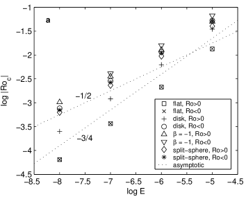
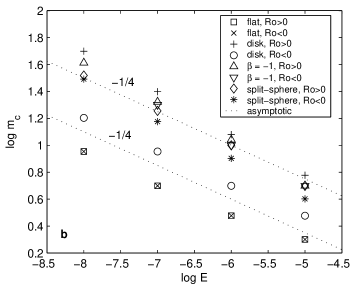
Figure 11: Critical Rossby number (a) and critical wavenumber (b) for various geometries. Dotted lines indicate the asymptotic exponent obtained in §V.1.2.

The critical wave-number data shows that the evolution of $m_{c}$ follows an $E^{1/4}$ law, for both flat and non-flat cases, as expected from the asymptotic study (§V.1). For the flat geometry, there is no difference between positive and negative Rossby number. The split-sphere setup, the $\beta=-1$ case and the disk geometry for $Ro>0$ have comparable critical wave-numbers.

The flat geometry has much lower critical wave-numbers and Rossby numbers. From figure 5d we also see that the first unstable mode is totally symmetric when changing the sign of Ro. It is also different from all the other cases (a,b and c) which present important slopes. The disk geometry seem to be a hybrid case between flat and non-flat geometry : From 5c, the spatial structure for $\mbox{{Ro}}>0$ is very much like the split-sphere setup, whereas for $Ro<0$ it seems to be somewhere in between split-sphere and flat geometry. The figure 11b confirm this, with a critical wave-number between flat and non-flat. This is because the $Ro<0$ instability develops in the flat inner region. On the other hand, figure 11a shows a critical Rossby number for $Ro<0$ very close to the split-sphere arrangement, whereas the $Ro>0$ seems to follow rather a slope-like $E^{3/4}$ law, even if the threshold is significantly higher than for the flat container.

VI Comparison with experiments

VI.1 Flat container

We reproduce numerically the constant depth experiments done by Früh & Read (1999). The results of our linear calculation for the threshold are significantly lower than the experimental ones, but are in good agreement with the theory of Niino & Misawa (1984). The critical wave-length is in good agreement as shown in table 2.

To explain the discrepancy between experiment and theory, Früh & Read (1999) invoke the lack of the inner $E^{1/3}$ layer in the modeling of Niino & Misawa (1984), which is also missing in this QG-model.

$$\begin{array}[]{ccccc}E&\mbox{{Ro}}_{c}^{F}&m_{c}^{F}&\mbox{{Ro}}_{c}^{S}&m_{c}^{S}\\ 1.1\,10^{-5}&0.044&6\textrm{-}8&0.021&6\\ 8.3\,10^{-6}&0.032&6\textrm{-}8&0.017&6\\ 5.6\,10^{-6}&0.025&6\textrm{-}8&0.013&7\\ \end{array}$$

Table 1: Comparison between the experimental results of Früh & Read (1999) (denoted by $.^{F}$) and the numerical results we obtain ($.^{S}$) for the stability threshold.

$$\begin{array}[]{ccccc}E&\mbox{{Ro}}_{c}^{N}&m_{c}^{N}&\mbox{{Ro}}_{c}^{S}&m_{c}^{S}\\ 3.0\,10^{-5}&0.050&5\textrm{-}6&0.048&5\\ 6.0\,10^{-6}&0.015&7\textrm{-}9&0.0145&8\\ \end{array}$$

Table 2: Comparison between the experimental results of Niino & Misawa (1984) (denoted by $.^{N}$) and the numerical results we obtain ($.^{S}$)for the stability threshold.

We also reproduce numerically the experiments of Niino & Misawa (1984), which has the particularity of having differential rotation only at the bottom of the tank, while the top is rotating at the mean angular velocity. Results are reported in table 2 and agree surprisingly well with the original experimental data, as did their numerical calculations.

VI.2 Spherical shell geometry

The case of a spherical shell is quite singular : $\beta$ has opposite sign for $r<r_{0}$ and $r>r_{0}$, and the magnitude of $\beta$ is much higher for $r<r_{0}$. This implies that Rossby waves travel in opposite directions in these two regions. For positive Ro, the instability may develop either in the $r>r_{0}$ region or in the $r<r_{0}$ one (see §IV.1 and fig. 6). In both directions the depth is decreasing, but from eq. 22 we know that the instability will appear in the outer region ($r>r_{0}$) where the magnitude of $\beta$ is lower. However, for negative Ro there is no deeper region around the shear layer, where the instability may be amplified by $\beta$-effect, so that we expect the threshold to be much higher and maybe the instability to be of a different kind, as the very small azimuthal wave-number observed by Hollerbach (2003) may suggest.

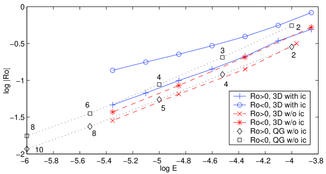
Figure 12: Critical Rossby numbers obtained by Hollerbach (2003, summary of his fig. 4 and 8a) showing the impact of the slope on the stability threshold. We also plotted the corresponding results obtained with our QG-model (basic state shear layer obtained with an inner core, instabilities computed without) including the critical mode. When removing the inner core (ic), the threshold drops, and positive and negative Rossby numbers get closer. Our QG-model is close to the fully 3D results of Hollerbach

We reported on figure 12 the data found in his paper. To check the effect of the geometry, he computed the basic-state shear layer in a spherical shell geometry, then took the profile obtained at mid-depth and extended it to all $z$, generating a $z$-invariant profile in a full sphere (see Hollerbach, 2003, §5). He finally computed the instabilities of that flow. By artificially removing the inner sphere (and by that way loosing the singular geometrical property described above), Hollerbach recovers stability thresholds very close to the $\mbox{{Ro}}>0$ case, which is much less modified by this process, for it is anyway controlled by the moderate slopes of the outer sphere.

We repeated exactly the same procedure with our QG-model : we computed the basic state shear layer with an inner-core ($r_{0}=0.35$), and then computed the stability threshold of this velocity profile in a full sphere geometry (without inner core). The results are compared with the 3D computations of Hollerbach on figure 12. For $\mbox{{Ro}}<0$, the QG-model gives thresholds about $30\%$ higher, and only $6\%$ higher for $\mbox{{Ro}}>0$. The critical modes obtained are also in very good agreement.

This geometrical singularity also prevents any attempt to compute the instabilities of the spherical shell setup with a QG-model. We used the dynamo benchmark code described by Christensen et al. (2001) to perform a fully 3D numerical calculation at $E=10^{-4.5}$. The critical Rossby number we find $\mbox{{Ro}}_{c}=0.16$ is in very good agreement with the experimental one and with the numerical results of Hollerbach (2003) as shown in figure 1.

VI.3 Experimental study

VI.3.1 Experimental setup

Figure 13 shows a sketch of the experimental set-up we use to study the onset of instability of the Stewartson layer. It consists of a plexiglass ellipsoid put in rotation by a brushless motor along its minor axis with a controlled angular velocity $\Omega_{0}$. The working fluid is water. On the axis of rotation a shaft associated to a step motor can drive either an inner core or two disks. Exact dimensions are reported in fig. 13 and further details can be found in Noir et al. (2003).

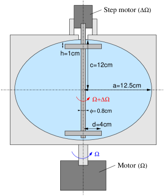
Figure 13: Sketch of the experimental setup with disks geometry. Spherical shell geometry is obtained by replacing the disks by a sphere (4cm radius) on the inner rotating axis.

To determine the stability threshold, we use a flake solution (Kalliroscope AQ 1000) and illuminate our container with a light sheet in a plane including the rotation axis. Variations of brightness allow us to visualize the shear-field in the illuminated plane. When the shear-field is steady, we assume that the flow is stable, and when the shear becomes unsteady (oscillations in time), the flow is unstable. Two pictures of the observed patterns are shown on figure 14, showing that the features of the flow are aligned with the rotation axis. The thin bright and dark columns appear at the onset and are blinking, showing the advection of the pattern of alternating vortices. Our visual determination shown in figure 1 is in good agreement with the numerical calculations of Hollerbach (2003). This makes us confident in the reliability of the optical method.

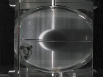
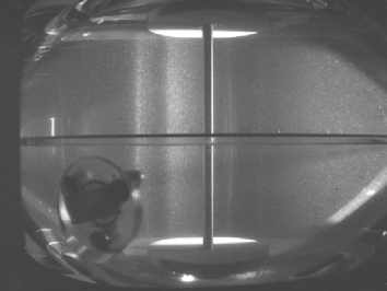
Figure 14: Instabilities near the threshold as seen in our experiments (for $E\simeq 10^{-5}$). The vertical shaft is along the rotation axis. The features shown by the flakes are vertical, supporting the QG-approximation for our model.

VI.3.2 Experimental results

The threshold is obtained for different values of the Ekman number with the two geometries (inner core or two disks) for prograde differential rotation. Results for the stability threshold are summarized in figure 15 and quantitative data are reported in tables C.3 and C.4

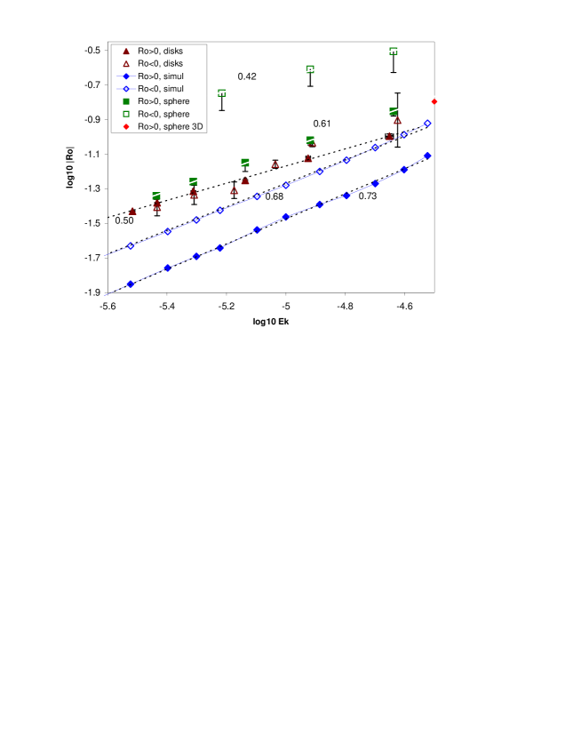
Figure 15: Experimental determination of the stability threshold for two geometries, compared with the numerical calculations using a quasi-geostrophic model. sphere 3D is computed with a fully 3D model. The negative differential rotation data are not well defined. The numbers are the slopes of the linear fits.

Note that in the case of negative differential rotation, we were not able to determine accurately a stability threshold. In some experiments hysteresis appeared, correlated with the apparition of air bubbles in the tank. We have also observed very low frequency oscillation is some cases. We do not completely understand these results. For the disks the data are not even on a straight line. This may be correct, as the numerical simulations also show some oscillations, due to the integer nature of the azimuthal wave number (see fig. 15).

The disk case seems to agree with the $E^{1/2}$ scaling, whereas the sphere case is significantly steeper. However with only one decade of data, and for such high Ekman numbers, we do not expect the asymptotic laws to hold.

The numerical calculations for the disk model (see also §V.3.2), also shown in figure 15 try to mimic the experimental setup : it is a split-sphere with flat polar caps with no height jump (we cannot model discontinuities in the height of the container).

The spherical-shell experiments are in agreement with the numerical calculations of Hollerbach (2003), as shown on figure 1. The strong difference between positive and negative differential rotation is explained by the geometrical properties of this setup, as discussed above.

VII Conclusion and Discussion

In this study, we give some insight into the instability of a Stewartson shear layer in the very low Ekman regime. The QG-model with the pseudo-stream function formalism is designed for finite slopes as it handles the mass conservation correctly. Despite failing to describe the $E^{1/3}$-layer, it has proved to be a valuable tool for numerical experiments to study very low Ekman numbers. It can also be used for non-linear calculations as long as the quasi-geostrophic hypothesis stands, and may be thus useful for other ocean and planetary interior models.

At very low Ekman numbers $E<10^{-6}$, we report an interesting radial structure, comparable to the one exhibited in the thermal instability case by Dormy et al. (2003). However, if the global structure of the flow is quite similar to the spiralling thermal convection flow in a rapidly rotating spherical shell, the radial extension of the instability is surprisingly independent of the Ekman number.

Our model allows us to compare flat top and bottom geometries with varying depth containers. Two different stabilizing processes are at work, leading to different balances and scalings for the threshold : for flat containers the Busse (1968) $E^{3/4}$ scaling applies, whereas with a slope a $\beta E^{1/2}$ scaling is predicted. This is supported by numerical simulations for different geometries, and the following table summarizes the different cases for the instability of a Stewartson layer :

geometry	$\mbox{{Ro}}_{c}$	sign of Ro	$m_{c}$	$f_{c}$	comment
$\beta=0$	$E^{3/4}$	$\mbox{{Ro}}_{c}^{+}=-\mbox{{Ro}}_{c}^{-}$	$E^{-1/4}$	$0$ ?	$Re_{c}=Cte$, Kelvin-Helmholtz-like
constant $\beta\neq 0$	$\beta E^{1/2}$	$\mbox{{Ro}}_{c}^{+}\simeq-\mbox{{Ro}}_{c}^{-}$	$E^{-1/4}$	$E^{1/4}$	curvature effect, Rossby wave
variable $\beta$	$\beta E^{1/2}$	$\mbox{{Ro}}_{c}^{+}\neq-\mbox{{Ro}}_{c}^{-}$	$E^{-1/4}$	$E^{1/4}$	spiralized Rossby wave
height jump	?	not symmetric	$E^{-1/4}$	?	QG-model breaks down

Hollerbach (2003) studied the difference between positive and negative Rossby numbers, and pointed out that the geometry is the crucial feature, through the radial derivative of the height of the container. The numerical calculations he made shed some light on the dramatic changes in the critical mode when switching from positive to negative Rossby numbers observed in some real experiments. However, ignoring the Rossby wave processes at work in varying depth containers, he misunderstood his numerical results.

As we demonstrated in this paper, all the geometrical effects are due to a fundamental symmetry breaking in the Rossby wave propagation mechanism : depending on the sign of Ro and $\beta$, the instability will develop on one side of the shear layer or the other. This symmetry breaking happens with any geometry, without the need for abrupt changes in the height of the container (even though this asymmetry will be magnified by such discontinuities). Furthermore, the spherical shell setup is singular : when $\mbox{{Ro}}<0$, the Rossby wave instability cannot develop on either side of the shear layer, leading to the singular results observed in this configuration. Within this framework, the recent results of Hollerbach (2003) may be interpreted correctly.

What still remains unclear is the nature of the instability in that particular case (spherical-shell and $\mbox{{Ro}}<0$). Is it just a Rossby wave that needs much stronger forcing to grow, or another type of instability with significant 3D effects ? This is even more annoying because this geometry is of geophysical interest for gaseous planets or planetary interiors. It is also the geometry used in the sodium experiment presented by Cardin et al. (2002), aimed at the study of induction processes in this type of flow, which are suspected to be able to drive a dynamo. In addition, the non-linear and turbulent regimes have to be investigated, by means of numerical calculations and quantitative velocity measurement in experiments. It is clear that we need experiments at lower Ekman numbers, especially for spherical shells.

Appendix A Ekman Pumping in a sphere

The Ekman pumping flow is given by Greenspan (1968)

$$\left.{\mbox{$u$}}.{\mbox{$n$}}\right|_{\pm L}=-\frac{E^{1/2}}{2}{\mbox{$n$}}.{\mbox{$\nabla$}}\wedge\left(\frac{{\mbox{$n$}}\wedge{\mbox{$u$}}\pm{\mbox{$u$}}}{\sqrt{\left|{\mbox{$n$}}.{\mbox{$e_{z}$}}\right|}}\right)$$ (28)

with $n$ the outward unit vector normal to the surface and $u$ the velocity jump between the geostrophic interior and the boundaries. This Ekman pumping flow is the next order term in the $E^{1/2}$ development, and is deduced from the quasi-geostrophic, $0$-order flow. However, it has a dynamic action on that flow, and is thus important for the dynamics of the system. For simplicity we assume that the boundaries are at rest in the rotating frame. It is straightforward to apply the result to moving boundaries by replacing the velocity by the jump in velocity.

A.1 Spherical coordinate system

We can separate this

$$-\frac{1}{2}E^{1/2}\left(\underbrace{{\mbox{$n$}}.{\mbox{$\nabla$}}\wedge\left(\frac{{\mbox{$n$}}\wedge{\mbox{$u$}}}{\sqrt{\left|{\mbox{$n$}}.{\mbox{$e_{z}$}}\right|}}\right)}_{a}\pm\underbrace{{\mbox{$n$}}.{\mbox{$\nabla$}}\wedge\left(\frac{{\mbox{$u$}}}{\sqrt{\left|{\mbox{$n$}}.{\mbox{$e_{z}$}}\right|}}\right)}_{b}\right)$$

We now use the spherical coordinate system $(\rho,\theta,\phi)$ to develop that expression, because it is the natural one for that boundary layer (${\mbox{$n$}}={\mbox{$e_{\rho}$}}$). Term $a$ reduces to

$$a=\left|\cos\theta\right|^{-1/2}\left(\pm\frac{\left|\tan\theta\right|}{2\rho}u_{\theta}-\frac{\partial u_{\rho}}{\partial\rho}-\frac{2}{\rho}u_{\rho}\right)$$

and term $b$ can be written as

$$b=\left|\cos\theta\right|^{-1/2}\left(\pm\frac{\left|\tan\theta\right|}{2\rho}u_{\phi}+\omega_{\rho}\right)$$

On the boundary, we have $\rho=1$, and so

$$\left.{\mbox{$u$}}.{\mbox{$n$}}\right|_{\pm L}=\frac{E^{1/2}}{2\left|\cos\theta\right|^{1/2}}\left(\frac{\left|\tan\theta\right|}{2}\left(\pm u_{\theta}-u_{\phi}\right)\>\pm\omega_{\rho}\>-2u_{\rho}-\frac{\partial u_{\rho}}{\partial\rho}\right)$$ (29)

A.2 QG-model flow

We now assume the use of our QG approximation described in §II. We need to translate 29 into cylindrical coordinate system $(r,\phi,z)$. We have

$$\rho\sin\theta=r \rho\cos\theta=z$$

$$u_{\theta}=u_{r}\cos\theta-u_{z}\sin\theta u_{\rho}=u_{r}\sin\theta+u_{z}\cos\theta$$

$$\frac{\partial}{\partial\rho}=\frac{\partial r}{\partial\rho}\frac{\partial}{\partial r}+\frac{\partial z}{\partial\rho}\frac{\partial}{\partial z}=\sin\theta\frac{\partial}{\partial r}+\cos\theta\frac{\partial}{\partial z}$$

Furthermore, $u_{r}$ and $u_{\phi}$ are $z$-independent, and $u_{z}$ is a linear function of $z$ (see section II.3) :

$$u_{z}=z\>\frac{-r}{1-r^{2}}\,u_{r}(r,\phi)$$ (30)

We find

$$\frac{\partial u_{\rho}}{\partial\rho}=\frac{-2r}{1-r^{2}}u_{r}$$ (31)

We also need to develop $\omega_{\rho}$ :

$$\omega_{\rho}=\omega_{z}\cos\theta+\omega_{s}\sin\theta$$

where $\omega_{r}$ is given by

$$\omega_{r}=\frac{1}{r}\frac{\partial u_{z}}{\partial\phi}=\frac{-z}{1-r^{2}}\frac{\partial u_{r}}{\partial\phi}$$

and finally

$$\left.{\mbox{$u$}}.{\mbox{$n$}}\right|_{\pm L} = \frac{E^{1/2}}{2(1-r^{2})^{1/4}}\left(\frac{-r}{2(1-r^{2})^{1/2}}u_{\phi}+\frac{5}{2}\frac{r}{1-r^{2}}u_{r}\right.$$ (32)

$$-\left.(1-r^{2})^{1/2}\left(\omega_{z}-\frac{r}{1-r^{2}}\frac{\partial u_{r}}{\partial\phi}\right)\right)$$

This expression can be treated just like the $0$-order no-slip boundary condition :

$$\left.{\mbox{$u$}}.{\mbox{$n$}}\right|_{\pm L}=ru_{r}\pm\sqrt{1-r^{2}}u_{z}$$

from which we deduce $u_{z}$ at the top and bottom boundary

$$\left.\pm u_{z}\right|_{\pm L}=\left(1-r^{2}\right)^{-1/2}\left(\left.{\mbox{$u$}}.{\mbox{$n$}}\right|_{\pm L}-ru_{r}\right)$$

and from the linear $z$-dependence of $u_{z}$ we obtain

$$\frac{\partial u_{z}}{\partial z} = \frac{E^{1/2}}{2(1-r^{2})^{3/4}}\left(-\omega_{z}+\frac{r}{1-r^{2}}\left(\frac{\partial u_{r}}{\partial\phi}-\frac{1}{2}u_{\phi}\right)-\frac{5r}{2(1-r^{2})^{3/2}}u_{r}\right)$$

$$+\frac{-r}{1-r^{2}}u_{r}$$

$$= E^{1/2}.P(u_{r},u_{\phi},r)+\beta u_{r}$$

It has to be emphasized that this results from a development in $E^{1/2}$, which is no more valid when approaching the equator.

A.3 Validity

In the expression A.2, we have an order $E^{1/2}$ and order $1$ term. The development is no more valid when these two terms are of the same order of magnitude. Setting $r=1-\epsilon$, we have $1-r^{2}\sim 2\epsilon$. Keeping the dominant terms in $1/\epsilon$, the limit of validity is given by

$$\frac{E^{1/2}}{2(2\epsilon)^{3/4}}\frac{5}{2}\frac{1}{(2\epsilon)^{3/2}}u_{r}\sim\frac{1}{2\epsilon}u_{r}$$

from which we get

$$\epsilon\sim\frac{1}{2}\left(\frac{5}{4}\right)^{4/5}E^{2/5}$$ (34)

which shows the $E^{2/5}$ singularity on the equator (see Roberts & Stewartson, 1963). The angular extension is easily obtained from geometrical considerations :

$$s=\cos\delta\theta\sim 1-\delta\theta^{2}/2\sim 1-\epsilon$$

so that $\delta\theta=(2\epsilon)^{1/2}$ and

$$\delta\theta\sim E^{1/5}$$ (35)

Appendix B A simple model for the radial scaling

B.1 Approximations and assumptions

In figure 5abc the perturbation of the shear layer spreads across the whole volume whereas in the flat container case (fig. 5d) or even the thermal convection case in a sphere (see Dormy et al., 2003), it is radially localized. In this section we derive a simple heuristic model that predict all these properties outside the Stewartson shear layer.

To simplify our study, we make a few approximations :

• we neglect the curvature;

• we drop the viscous dissipation term, but keep the Ekman friction;

• we assume small forcing, ignoring the local vorticity term.

The curvature may be negligible if the scales involved are small enough. Looking at the results from section V.1, we expect the scales to shrink while lowering the Ekman number. Thus, we replace the angular variable $\phi$ by $y$. Dropping the viscous term lowers the order of the differential equation and makes it easier to handle. Numerical simulations with no viscous term or an artificially weakened viscous term show that the structure stays very similar. In addition, the threshold is expected to be only slightly affected in the asymptotic regime. This is because the Ekman friction is also a dissipative term. Finally, we can neglect the local vorticity term because in the linear stability case it is a higher order effect, as shown in section V.2. We end up with

$$\frac{\partial\omega}{\partial t}+\mbox{{Ro}}\left(U\frac{\partial\omega}{\partial y}+u_{r}\frac{\partial\Omega}{\partial r}\right)=2\left\langle\frac{\partial u_{z}}{\partial z}\right\rangle$$ (36)

The expression of the Ekman friction involves several terms. We will only keep the vorticity contribution, so that

$$\left\langle\frac{\partial u_{z}}{\partial z}\right\rangle\simeq\beta u_{r}-\alpha E^{1/2}\omega$$ (37)

where $\alpha$ is the geometrical factor for the Ekman friction term, and for a sphere $\alpha=1/2(1-r^{2})^{-3/4}$ (see eq. A.2).

We now assume a perturbation of the form

$$\Psi(r,y,t)=\psi(r)e^{i\left(ky-\omega t\right)}$$

and we obtain

$$\left(-i\omega+\mbox{{Ro}}Uik+E^{1/2}\alpha\right)\left(k^{2}-\frac{\partial^{2}}{\partial{r}^{2}}\right)\psi+\left(\mbox{{Ro}}\frac{\partial\Omega}{\partial r}-2\beta\right)ik\psi=0$$ (38)

In a more convenient form, we can write

$$\frac{\partial^{2}\psi}{\partial{r}^{2}}=k^{2}\left(1+\frac{1}{k}\frac{\left(2\beta-\mbox{{Ro}}\frac{\partial\Omega}{\partial r}\right)\left(\omega-\mbox{{Ro}}Uk-iE^{1/2}\alpha\right)}{\left(\omega-\mbox{{Ro}}Uk\right)^{2}+E\alpha^{2}}\right)\psi$$ (39)

B.2 Outer part, large $\beta$

In the outer part the basic state velocity profile $U$ is vanishing, as well as $\frac{\partial\Omega}{\partial r}$. This simplifies the previously established relation 39 :

$$\frac{\partial^{2}\psi}{\partial{r}^{2}}=k^{2}\left(1+\frac{2\beta}{k}\>\frac{\omega-iE^{1/2}\alpha}{\omega^{2}+E\alpha^{2}}\right)\psi$$ (40)

In the case of small Ekman number, $E\alpha^{2}$ is negligible compared to $\omega^{2}\sim E^{1/2}$, but we have to keep the small imaginary part. We now set

$$\gamma=k\left|1+\frac{2\beta}{k\omega}\right|^{1/2}$$

If $\left|2\beta\right|\gg 1$, we can rewrite 40 as

$$\frac{\partial^{2}\psi}{\partial{r}^{2}}=-\gamma^{2}\left(1-\frac{2i\beta E^{1/2}\alpha}{k\omega^{2}+2\beta\omega}\right)\psi$$ (41)

and the solution for constant $\alpha$ and $\beta$ is of the form

$$\psi=\exp\left(\pm\gamma\frac{\beta E^{1/2}\alpha}{k\omega^{2}+2\beta\omega}r\right)\>\exp(\pm i\gamma r)$$

This implies a rapid oscillation of typical length scale $\gamma$

$$\gamma\sim k\sqrt{\left|2\beta\right|}$$ (42)

modulated by a slow exponential decay with typical length scale $\delta$ given by

$$\delta\sim\gamma^{-1}E^{-1/2}\alpha^{-1}\omega$$ (43)

Inside this envelope, the radial length scale $\gamma^{-1}$ of the perturbation decreases when $\beta$ increases. It corresponds to the spiralling of the Rossby wave observed for variable $\beta$ (see fig. 5bc)

Using the scalings for the Stewartson layer instability $k\sim E^{-1/4}$ and $\omega\sim E^{1/4}$, relation 43 leads to

$$\delta\sim\left(2\left|\beta\right|\right)^{-1/2}\alpha^{-1}E^{0}$$ (44)

which implies that the radial extension of the perturbation is independent of $E$. This is a fundamental difference with the thermal convection case investigated by Yano (1992) and Jones et al. (2000) where the scaling $k\sim E^{-1/3}$ and $\omega\sim E^{1/3}$ implies

$$\delta\sim\left(2\left|\beta\right|\right)^{-1/2}\alpha^{-1}E^{1/6}$$ (45)

which corresponds to a slowly decaying radial extension when decreasing $E$.

B.3 Inner part, small $\beta$

The inner part behaves exactly as the outer one, replacing $\omega$ by $\omega-\mbox{{Ro}}Uk$. For a spherical shell it corresponds to the small $\beta$ case.

If $\left|2\beta\right|<k\omega$, we can rewrite 40 as

$$\frac{\partial^{2}\psi}{\partial{r}^{2}}=\gamma^{2}\left(1-\frac{2i\beta E^{1/2}\alpha}{k\omega^{2}+2\beta\omega}\right)\psi$$ (46)

which actually exchanges the length scale of the exponential decay and of the oscillation compared to the outer region. The solution for constant $\alpha$ and $\beta$ is then

$$\psi=\exp(\pm\gamma r)\>\exp\left(\mp i\gamma\frac{\beta E^{1/2}\alpha}{k\omega^{2}+2\beta\omega}r\right)$$

which is an exponential decay of characteristic length $\gamma^{-1}$, inside which there are much larger length scale oscillations, which cannot be detected.

For the Rossby wave, we have $\omega\sim k^{-1}$, so that $\gamma\sim k$, with a correction independent of $E$. This shows that in the small $\beta$ case the critical mode has a radial extension comparable to its azimuthal scale.

Appendix C Stability threshold data

C.1 Split-sphere stability threshold

Linear stability threshold values for different Ekman numbers $E$. NR denotes the number of radial grid points used for the calculation. These values where obtained by QG numerical calculations with no-slip boundary conditions and including Ekman friction.

$$\begin{array}[]{ccccc}E&\mbox{{Ro}}_{c}&m_{c}&\omega_{c}&\textrm{NR}\\ \hline\cr 10^{-5}&4.017\,10^{-2}&5&9.886\>10^{-2}&300\\ &-5.122\,10^{-2}&4&-3.495\>10^{-2}&\\ 10^{-6}&9.505\,10^{-3}&10&5.428\>10^{-2}&400\\ &-11.08\,10^{-3}&8&-2.060\>10^{-2}&\\ 10^{-7}&2.326\,10^{-3}&18&2.689\>10^{-2}&600\\ &-2.674\,10^{-3}&15&-0.999\>10^{-2}&\\ 10^{-8}&6.314\,10^{-4}&33&1.388\>10^{-3}&800\\ &-7.018\,10^{-4}&31&-6.446\>10^{-3}&\\ 10^{-9}&1.821\,10^{-4}&63&7.505\>10^{-3}&1200\\ &-1.938\,10^{-4}&61&-3.844\>10^{-3}&\\ 10^{-10}&5.357\,10^{-5}&121&4.128\>10^{-3}&1500\\ &-5.543\,10^{-5}&119&-2.317\>10^{-3}&\end{array}$$

C.2 Boundary conditions and viscosity dependence

Comparison between $\mbox{{Ro}}_{c}$ of different numerical models for the split-sphere geometry. Values are the $\mbox{{Ro}}_{c}$ obtained by a model divided by the reference $\mbox{{Ro}}_{c}$ (ns,ep) for $\mbox{{Ro}}>0$ at a given Ekman number. The models are referenced by ns and fs respectively for no-slip and free-slip boundary conditions, ep for the Ekman pumping, dv for horizontal divergence and vs for bulk viscosity; $\times 2$ stands for calculation with doubled number of radial grid points. A $0$ denotes the absence of this feature.

$$\begin{array}[]{ccccccc}E&ns,ep&ns,ep0&fs,ep0&ns,ep,dv0&ns,ep,vs0&ns,ep,\times 2\\ \hline\cr 10^{-6}&1.0&0.86&0.87&0.995&0.64&0.999\\ 10^{-7}&1.0&0.91&0.91&1.001&0.72&1.000\\ 10^{-8}&1.0&0.94&0.94&1.002&0.78&1.000\\ \end{array}$$

C.3 Spherical shell experimental threshold

Stability threshold experimental data obtained for the spherical shell geometry, in water ($\nu=10^{-6}\mathrm{~{}m^{2}/s}$). See §VI.3.1 for details about the experimental setup.

$$\begin{array}[]{ccc}E&\textrm{stable}\>\mbox{{Ro}}&\textrm{unstable}\>\mbox{{Ro}}\\ \hline\cr 3.51\;10^{-5}&0.175&0.183\\ 2.30\;10^{-5}&0.135&0.141\\ 1.21\;10^{-5}&9.29\;10^{-2}&9.56\;10^{-2}\\ 7.30\;10^{-6}&6.93\;10^{-2}&7.10\;10^{-2}\\ 4.88\;10^{-6}&5.30\;10^{-2}&5.52\;10^{-2}\\ 3.67\;10^{-6}&4.48\ 10^{-2}&4.56\;10^{-2}\\ \hline\cr 2.30\;10^{-5}&-0.302&-0.313\\ 1.21\;10^{-5}&-0.232&-0.246\\ 6.09\;10^{-6}&-0.165&-0.179\\ \end{array}$$

C.4 Disks experimental threshold

Stability threshold experimental data obtained for the disks geometry, in water ($\nu=10^{-6}\mathrm{~{}m^{2}/s}$). See §VI.3.1 for details about the experimental setup.

$$\begin{array}[]{ccc}E&\textrm{stable}\>\mbox{{Ro}}&\textrm{unstable}\>\mbox{{Ro}}\\ \hline\cr 2.23\;10^{-5}&10.1\;10^{-2}&11.1\;10^{-2}\\ 1.19\;10^{-5}&7.53\;10^{-2}&8.06\;10^{-2}\\ 7.30\;10^{-6}&5.61\;10^{-2}&5.94\;10^{-2}\\ 4.88\;10^{-6}&4.86\;10^{-2}&5.08\;10^{-2}\\ 3.68\;10^{-6}&4.17\;10^{-2}&4.33\;10^{-2}\\ 3.04\;10^{-6}&3.72\;10^{-2}&3.99\;10^{-2}\\ \hline\cr 2.38\;10^{-5}&-12.5\;10^{-2}&-15.0\;10^{-2}\\ 1.23\;10^{-5}&-9.27\;10^{-2}&-9.53\;10^{-2}\\ 9.21\;10^{-6}&-6.95\;10^{-2}&-7.14\;10^{-2}\\ 6.70\;10^{-6}&-4.92\;10^{-2}&-5.20\;10^{-2}\\ 4.91\;10^{-6}&-4.63\;10^{-2}&-4.93\;10^{-2}\\ 3.68\;10^{-6}&-3.93\;10^{-2}&-4.00\;10^{-2}\\ \end{array}$$

References

- Aubert et al. (2003) Aubert, J., Gillet, N. & Cardin, P. 2003 Quasigeostrophic models of convection in rotating spherical shells. Geochem. Geophys. Geosyst. 4(7), 1052.
- Brito et al. (2004) Brito, D., Aurnou, J. & Cardin, P. 2004 Turbulent viscosity measurements relevant to planetary core mantle dynamics. Phys. Earth Planetary Interiors 141, 3–8.
- Busse (1968) Busse, F. H. 1968 Shear flow instabilities in rotating systems. J. Fluid Mech. 33, 577–589.
- Busse (1970) Busse, F. H. 1970 Thermal instabilities in rapidly rotating systems. J. Fluid Mech. 44, 441–460.
- Cardin et al. (2002) Cardin, P., Brito, D., Jault, D., Nataf, H.-C. & Masson, J.-P. 2002 Towards a rapidly rotating liquid sodium dynamo experiment. Magnetohydrodynamics 38, 177–189.
- Christensen et al. (2001) Christensen, U., Aubert, J., Cardin, P., Dormy, E., Gibbons, S., Glatzmaier, G., Grote, E., Honkura, Y., Jones, C., Kono, M., Matsushima, M., Sakuraba, A., Takahashi, F., Tilgner, A., Wicht, J. & Zhang, K. 2001 A numerical dynamo benchmark. Phys. Earth Planetary Interiors 128, 25–34.
- Dormy et al. (1998) Dormy, E., Cardin, P. & Jault, D. 1998 MHD flow in a slightly differentially rotating spherical shell, with conducting inner core, in a dipolar magnetic field. Earth. Planet. Sc. Lett. 160, 15–30.
- Dormy et al. (2003) Dormy, E., Soward, A., Jones, C., Jault, D. & Cardin, P. 2003 The onset of thermal convection in rotating spherical shells. accepted for publication in JFM .
- Früh & Read (1999) Früh, W.-G. & Read, P. L. 1999 Experiments on a barotropic rotating shear layer. part 1. instability and steady vortices. J. Fluid Mech. 383, 143–173.
- Greenspan (1968) Greenspan, H. P. 1968 The theory of rotating fluids. Breukelen Press.
- Hide & Titman (1967) Hide, R. & Titman, C. W. 1967 Detached shear layers in a rotating fluid. J. Fluid Mech. 29, 39–60.
- Hollerbach (2003) Hollerbach, R. 2003 Instabilities of the Stewartson layer part 1. the dependence on the sign of Ro. J. Fluid Mech. 492, 289–302.
- Jones et al. (2000) Jones, C. A., Soward, A. M. & Mussa, A. I. 2000 The onset of thermal convection in a rapidly rotating sphere. J. Fluid Mech. 405, 157–179.
- Kiss (2003) Kiss, A. E. 2003 A modified quasigeostrophic formulation for weakly nonlinear barotropic flow with large-amplitude depth variations. Ocean Model. 5, 171–191.
- van de Konijnenberg et al. (1999) van de Konijnenberg, J. A., Nielsen, A. H., Rasmussen, J. J. & Stenum, B. 1999 Shear-flow instability in a rotating fluid. J. Fluid Mech. 387, 177–204.
- Kuo (1949) Kuo, H. L. 1949 Dynamic instability of two-dimensional non-divergent flow in a barotropic atmosphere. J. Meteor. 6, 105–122.
- Moore & Saffman (1969) Moore, D. W. & Saffman, P. G. 1969 The structure of free vertical shear layers in a rotating fluid and the motion produced by a slowly rising body. Phil. T. R. Soc. Lond. A 264, 597–634.
- Niino & Misawa (1984) Niino, H. & Misawa, N. 1984 An experimental and theoretical study of barotropic instability. J. Atmos. Sci. 41, 1992–2011.
- Noir et al. (2003) Noir, J., Cardin, P., Jault, D. & Masson, J.-P. 2003 Experimental evidence of nonlinear resonance effects between retrograde precession and the tilt-over mode within a spheroid. Geophys. J. Int. 154, 407–416.
- Proudman (1956) Proudman, I. 1956 The almost-rigid rotation of viscous fluid between concentric spheres. J. Fluid Mech. 1, 505–516.
- Roberts & Stewartson (1963) Roberts, P. H. & Stewartson, K. 1963 On the stability of a Maclaurin spheroid of small viscosity. Astrophys. J. 137, 777–790.
- Stewartson (1957) Stewartson, K. 1957 On almost rigid rotations. J. Fluid Mech. 3, 17–26.
- Stewartson (1966) Stewartson, K. 1966 On almost rigid rotations. part 2. J. Fluid Mech. 26, 131–144.
- Yano (1992) Yano, J.-I. 1992 Asymptotic theory of thermal convection in rapidly rotating systems. J. Fluid Mech. 243, 103–131.
- Yano et al. (2003) Yano, J.-I., Talagrand, O. & Drossart, P. 2003 Outer planets: Origins of atmospheric zonal winds. Nature 421, 36.
- Zavala Sanson & van Heijst (2002) Zavala Sanson, L. & van Heijst, G. J. F. 2002 Ekman effects in a rotating flow over bottom topography. J. Fluid Mech. 471, 239–255.