Multilayer shallow-water model with stratification and shear

Abstract

The purpose of this paper is to present a shallow-water-type model with multiple inhomogeneous layers featuring variable linear velocity vertical shear and startificaion in horizontal space and time. This is achieved by writing the layer velocity and buoyancy fields as linear functions of depth, with coefficients that depend arbitrarily on horizontal position and time. The model is a generalization of Ripa’s (1995) single-layer model to an arbitrary number of layers. Unlike models with homogeneous layers the present model is able to represent thermodynamics processes driven by heat and freshwater fluxes through the surface or mixing processes resulting from fluid exchanges across contiguous layers. By contrast with inhomogeneous-layer models with depth-independent velocity and buoyancy, the model derived here can sustain explicitly at low frequency a current in thermal wind balance (between the vertical vertical shear and the horizontal density gradient) within each layer. In the absence of external forcing and dissipation, energy, volume, mass, and buoyancy variance constrain the dynamics; conservation of total zonal momentum requires in addition the usual zonal symmetry of the topography and horizontal domain. The inviscid, unforced model admits a formulation suggestive of a generalized Hamiltonian structure, which enables the classical connection between symmetries and conservation laws via Noether’s theorem. A steady solution to a system involving one Ripa-like layer and otherwise homogeneous layers can be proved formally (or Arnold) stable using the above invariants. A model configuration with only one layer has been previously shown to provide: a very good representation of the exact vertical normal modes up to the first internal mode; an exact representation of long-perturbation (free boundary) baroclinic instability; and a very reasonable representation of short-perturbation (classical Eady) baroclinic instability. Here it is shown that substantially more accurate overall results with respect to single-layer calculations can be achieved by considering a stack of only a few layers. A similar behavior is found in ageostrophic (classical Stone) baroclinic instability by describing accurately the dependence of the solutions on the Richardson number with only two layers.

Keywords.

Shallow water equations; inhomogeneous layers; stratification; shear; mixed layer dynamics and thermodynamics.

1 Introduction

1.1 Motivation

There is renewed interest to construct models for the study of the dynamics in the upper ocean (i.e., above the main thermocline, including the mixed layer) such that:

1. are capable of incorporating thermodynamic processes while maintaining the two-dimensional structure of the rotating shallow-water equations, a paradigm of ocean dynamics on scales longer than a few hours [Pedlosky, 1987]; and

2. preserve the geometric (generalized Hamiltonian) structure of the exact three-dimensional models from which they derive [Holm et al., 2002].

Property 1) promises fundamental understanding of ocean processes which are difficult—if not impossible—to be attained using ocean general circulation models. Property 2) enables applying a recent flow-topology-preserving framework [Holm, 2015] to build parametrizations [Cotter et al., 2020] of unresolvable submesoscale motions and this way investigating the contribution of these to transport at resolvable scales, a topic of active research [McWilliams, 2016].

1.2 Background

Back in the late 1960s and early 1970s and independently by various authors [O’Brien and Reid, 1967; Dronkers, 1969; Lavoie, 1972], the rotating shallow-water model was extended by allowing for horizontal and temporal variations of the density field, while keeping it as well as the velocity field independent of depth. In the simplest setting, e.g., with one active layer floating atop an abyssal layer of inert fluid, the resulting inhomogeneous-layer model enables the investigation of thermodynamic processes in the upper ocean driven by heat and freshwater fluxes across the surface. Due to the two-dimensional nature of the model, the computational coast involved in such an investigation is consideraably much lower than that produced by an ocean general circulation model [Anderson and McCreary, 1985; McCreary et al., 1997].

Following nomenclature introduced in Ripa [1995, hereinafter R95], we will refer to the model above as IL⁰, indicating that it represents an inhomogenous-layer model wherein fields are not allowed to vary in the vertical. The homogeneous-layer shallow-water model will be called HL. Additional, more recent terminology for the IL⁰ is “thermal rotating shallow-water model” [Warnerford and Dellar, 2013; Zeitlin, 2018], which emphasizes the ability of the IL⁰ to include (horizontal) gradients of temperature. The IL⁰ is also being called “Ripa model” in the literature [Dellar, 2003; Desveaux et al., 2015; Mungkasi and Roberts, 2016; Sanchez-Linares et al., 2016; Rehman et al., 2018; Britton and Xing, 2020], in recognition of Pedro Ripa’s contribution to its understanding [Ripa, 1993; 1994; 1996b; 1995; 1999]. We will reserve that to refer to the model generalized here, which was introduced in R95.

The assessment on the computational cost efficiency of the IL⁰ holds even when more than one active layer is considered [Schopf and Cane, 1983; McCreary and Kundu, 1988; McCreary et al., 1991; 2001; Zavala-Hidalgo et al., 2002] or when the abyssal layer is activated and rests over irregular topography [Beier, 1997; Beier and Ripa, 1999; Palacios-Hernández et al., 2002]. Furthermore, due the simplicity of the IL⁰ compared to the primitive equations for arbitrarily stratified fluid, referred to herein as IL^∞, it has facilitated conceptual understanding of basic aspects of the upper-ocean dynamics and thermodynamics [Ripa, 1997; 2001; Beron-Vera and Ripa, 2002; Ripa, 2003]. Due in part to this very important reason, namely, the possibility to gain insight that is difficult to attain with an ocean general circulation model, the IL⁰ has been recently revisited [Gouzien et al., 2017; Zeitlin, 2018; Lahaye et al., 2020; Holm et al., 2020].

A multilayer version of the IL⁰ was derived in Ripa [1993] and a low-frequency approximation was developed in Ripa [1996b]; cf. recent rederivations in Warnerford and Dellar [2013]; Holm et al. [2020]. The no-vertical-variation ansatz cannot be maintained under the exact dynamics produced by the IL^∞ when horizontal density gradients are present. The recipe used to keep the dynamical fields depth independent is to vertically average the horizontal pressure gradient. (Some authors [e.g., Fukamachi et al., 1995] postulate a turbulent momentum flux that exactly cancels the vertical variation of the horizontal pressure gradient, but this is no more than an ad-hoc hypothesis which sheds no light on the problem.) While this is clearly an approximation, Ripa [1993] showed that it does not spoil the integrals of motion and generalized Hamiltonian structure of the problem.

Furthermore, the IL⁰ possess a Lie–Poisson Hamiltonian structure [Dellar, 2003] and associated with it an Euler–Poincare variational formulation [Bröcker et al., 2018] wherein the Hamilton principle’s Lagrangian follows by vertically averaging that of the IL^∞ [Holm and Luesink, 2020]. When the equations of motion are derived in this formulation, there is a natural way to express three fundamental relations [Holm et al., 2002]. These are: 1) the Kelvin circulation theorem, 2) the advection equation for potential vorticity, and 3) an infinite family of conserved Casimir invariants (arising from Noether’s theorem for the symmetry of Eulerian fluid quantities under Lagrangian particle relabelling). The Euler–Poincare formulation provides a means to consistently introduce data-driven parameterizations of stochastic transport using the SALT (stochastic advection by Lie transport) algorithm [Holm, 2015; Holm and Luesink, 2020], enabling data assimilation in a geometry-preserving context.

The IL⁰ provides an attractive framework for applying the SALT algorithm to derive parameterizations for unresolved submesoscale motions in the upper ocean. Indeed, numerical simulations of the IL⁰ [Ochoa et al., 1998; Pinet and Pavía, 2000; Gouzien et al., 2017] tend to reveal small scale circulations that resemble quite well [Holm et al., 2020] submesoscale filament rollups often observed in satellite-derived ocean color images. Such submesoscale motions may be unresolvable in many computational simulations. The extent to which they contribute to fluid transport at resolvable scales is a subject of active investigation [McWilliams, 2016] that the SALT stochastic version of the IL⁰ may cast light on.

1.3 Limitations of the IL⁰

Despite the above geometric properties of the IL⁰, it has a number of less attractive aspects, which can be consequential for the production of small scale circulations in the model. Discussed in detail by Ripa [1999], these include:

1. In addition to the classical Poincare and Rossby waves, the IL⁰ represents variations of the thickness and density that do not change the vertical average of the pressure gradient [Ripa, 1995; 1996a]. This mode is not present in the IL^∞.

2. A uniform flow may be unstable [Fukamachi et al., 1995; Young and Chen, 1995; Ripa, 1996a]. A priori, this phenomenon seems to be something different than baroclinic instability. For instance, unlike Eady’s problem, it experiences an “ultraviolet divergence” in the sense that a short-wave cutoff is lacking.

3. Since the dynamical fields are kept depth independent within each layer, there is no explicit representation of the thermal wind balance, between the velocity vertical shear and the horizontal density gradient, which dominates at low frequency.

An important additional liminitation imposed by the depth independence of the dynamical fields, and particularly the buoyancy, is:

1. The IL⁰ cannot represent the restratification of the oceanic surface mixed layer resulting from ageostrophic baroclinic instability of lateral density gradients, which tend to slump from the horizontal to the vertical [Tandon and Garrett, 1994; Haine and Marshall, 1998; Boccaletti et al., 2007].

1.4 The IL¹

To cure the unwanted features of the IL⁰, R95 proposed the following improved closure to incorporate thermodynamic processes in a one-layer ocean model not restricted to low frequencies:

in addition to allowing arbitrary velocity and buoyancy variations in horizontal position and time, the velocity and buoyancy fields are also allowed to vary linearly with depth.

Ripa’s single-layer model, denoted IL¹, enjoys a number of properties which make it very promising. For instance:

1. The IL¹ represents explicitly the thermal wind balance which dominates at low frequency.

2. The free waves supported by the IL¹ (Poincaré, Rossby, midlatitude coastal Kelvin, equatorial, etc.) are a very good approximation to the first and second vertical modes in the exact model with unlimited vertical variation.

3. The IL¹ provides an exact representation of long-perturbation baroclinic instability and a very reasonable representation of short-perturbation baroclinic instability.

1.5 This paper

In this paper I present a generalization of the IL¹ to an arbitrary number of layers, including two possible (mathematically equivalent) vertical configurations (Sec. 2). The model obtained incorportaes additonal flexibility to treat more complicated problems than those that can be tackled with only one layer. With a single layer in a reduced-gravity setting mixed-layer processes can be minimally modeled. Including additional layers can lead to a more accurate representation of such processes. On the other hand, considering a stack of several layers atop an irregular bottom will enable investigating the influence of the ocean’s interior and even topographic effects. Several aspects of the gereneralized IL¹ are discussed in Sec. 3. These include: remarks on submodels derived from the generalized model as special cases (Sec. 3.1); the nature of the layer boundaries (Sec. 3.2); the model conservation laws (Sec. 3.3); a discussion on circulation theorems (Sec. 3.4); a formulation of the model suggstive of a generalized Hamiltonian structure (Sec. 3.5); a formal stability theorem (Sec. 3.6); results on vertical normal modes (Sec. 3.7) and on baroclinic instability (Sec. 3.8), both quasigeostrophic and ageostrophic, which demonstrate that improved performance with respect to the single-layer results can be attained by considering only a few more layers; and the incorporation of forcing in the model equations (Sec. 3.9). Section 4 closes the paper with some concluding remarks.

2 The multilayer IL¹

Consider a stack of $n$ active fluid layers with thickness $h_{i}(\mathbf{x},t),$ $i=1,\dotsc,n$, where $\mathbf{x}$ is horizontal position and $t$ sands for time (Figure 1). The geometry can be either planar or spherical; in the former case the vertical coordinate, $z$, is perpendicular to the plane, whereas in the latter it is radial. The total thickness is $h(\mathbf{x},t)=\sum_{j}h_{j}(\mathbf{x},t).$ The stack of inhomogeneous-density layers can be either limited from below by a rigid bottom, $z=h_{0}(\mathbf{x})$, or from above by a rigid lid, $z=-h_{0}(\mathbf{x}).$ The usual choice in the rigid lid case is $h_{0}\equiv 0$; however, laboratory experiments are often designed to have a nonhorizontal top lid. The remaining boundary in the rigid-bottom (resp., rigid-lid) configuration is a soft interface with a passive, infinitely thick layer of lighter (resp., denser) homogeneous fluid of density $\rho_{n+1}$. Although vacuum ($\rho_{n+1}\equiv 0$) is the typical setting in the rigid-bottom configuration, the choice $\rho_{n+1}\neq 0$ can be useful to study of deep flows over topography.

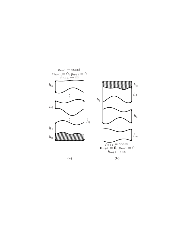
Figure 1: The two possible vertical configurations of the $n$-IL¹  are rigid bottom (a) and rigid lid (b). Within each layer the velocity and buoyancy fields not only vary arbitrarily with the horizontal position and time, but also linearly with depth.

A key element to generalize Ripa’s model is to define a scaled vertical coordinate $\sigma_{i}$ so as to vary linearly from $\pm 1$ at the base to $\mp 1$ at the top of the $i$th layer (Figure 2):

$$\pm z=:\tilde{h}_{i-1}(\mathbf{x},t)+\frac{1-\sigma_{i}}{2}h_{i}(\mathbf{x},t)=\nu_{i}(\mathbf{x},\sigma_{i},t),$$ (1)

where

$$\tilde{h}_{i}(\mathbf{x},t):=h_{0}(\mathbf{x})+\sum_{j=1}^{i}h_{j}(\mathbf{x},t)$$ (2)

[henceforth an upper (resp., lower) sign will correspond to the rigid-bottom (resp., rigid-lid) configuration]. The scaled vertical coordinate $\sigma$ defined in R95 according to

$$z=:h_{0}(\mathbf{x})+\frac{1}{2}(\sigma-1)h(\mathbf{x},t)=\nu(\mathbf{x},\sigma,t)$$ (3)

relates to the $i$th-layer scaled vertical coordinate $\sigma_{i}$ defined here through

$$\sigma=1-2\sum_{j=1}^{i-1}\frac{h_{j}}{h}+(1-\sigma_{i})\frac{h_{i}}{h}.$$ (4)

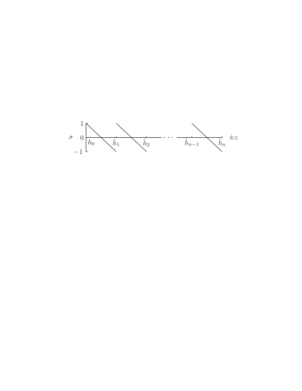
Figure 2: Vertical coordinate choice. Within each layer the rescaled vertical coordinate $\sigma$ varies linearly from $\pm 1$, at the base, to $\mp 1$, at the top. The upper (resp., lower) sign corresponds to the rigid-bottom (resp., rigid-lid) configuration of Figure 1.

Let an overbar denote vertical average within the $i$th layer:

$$\bar{a}_{i}(\mathbf{x},t):=\frac{1}{2}\int_{-1}^{+1}a(\mathbf{x},\sigma,t)\operatorname{d}\!{\sigma_{i}}=\frac{1}{2}\int_{-1}^{+1}a_{i}(\mathbf{x},\sigma_{i},t)\operatorname{d}\!{\sigma_{i}}.$$ (5)

Following R95 closely, the $i$th-layer horizontal velocity and buoyancy fields are written, respectively, as

$$\mathbf{u}_{i}(\mathbf{x},\sigma_{i},t) =\mathbf{\bar{u}}_{i}(\mathbf{x},t)+\sigma_{i}\mathbf{u}_{i}^{\sigma}(\mathbf{x},t),$$ (6a)

$$\vartheta_{i}(\mathbf{x},\sigma_{i},t) =\bar{\vartheta}_{i}(\mathbf{x},t)+\sigma_{i}\vartheta_{i}^{\sigma}(\mathbf{x},t),$$ (6b)

which can be regarded as a truncation of an expansion in orthogonal polynomials of $$\sigma_{i}$$ of the form

$$a_{i}(\mathbf{x},\sigma_{i},t)=\bar{a}_{i}(\mathbf{x},t)+\sigma_{i}a_{i}^{\sigma}(\mathbf{x},t)+\tfrac{1}{2}\left(\sigma_{i}^{2}-\tfrac{1}{3}\right)a_{i}^{\sigma\sigma}(\mathbf{x},t)+\tfrac{1}{6}\left(\sigma_{i}^{3}-\tfrac{3}{5}\sigma_{i}\right)a_{i}^{\sigma\sigma\sigma}(\mathbf{x},t)+\dotsc,$$ (7)

where $a_{i}^{\sigma}:=\overline{\partial_{\sigma_{i}}a_{i}},$ $a_{i}^{\sigma\sigma}:=\overline{\partial_{\sigma_{i}\sigma_{i}}a_{i}},$ etc. [Ripa, 1999]. The $i$th-layer buoyancy is defined as

$$\vartheta_{i}(\mathbf{x},\sigma_{i},t):=\pm g\,\frac{\rho_{i}(\mathbf{x},\sigma_{i},t)-\rho_{n+1}}{\rho_{\mathrm{r}}},$$ (8)

where the upper (resp., lower) sign corresponds to the rigid-bottom (resp., rigid-lid). Here, $g$ is gravity, $\rho_{i}(\mathbf{x},\sigma_{i},t)=\bar{\rho}_{i}(\mathbf{x},t)+\sigma_{i}\rho_{i}^{\sigma}(\mathbf{x},t)$ is the (variable) density in the $i$th layer, and $\rho_{\mathrm{r}}$ denotes the (constant) reference density used in the Boussinesq approximation. Physically admissible buoyancy values, i.e., everywhere positive and monotonically increasing (resp., decreasing) with depth in the rigid-bottom (resp., rig-lid) case, are such that

$$\bar{\vartheta}_{i}>\vartheta_{i}^{\sigma}>0,\quad\bar{\vartheta}_{i}-\bar{\vartheta}_{i+1}\geq\vartheta_{i}^{\sigma}+\vartheta_{i+1}^{\sigma}.$$ (9)

If $n_{i}^{2}(\mathbf{x},t)>0$ is the square of the instantaneous Brunt-Väisälä frequency within the $i$th layer, then note that

$$\vartheta_{i}^{\sigma}=\tfrac{1}{2}n_{i}^{2}h_{i}.$$ (10)

In order to obtain the equations for the $n$-layer version of Ripa’s model one must proceed as follows:

1. Substitute ansatz (6) in the inviscid, unforced, primitive equations (namely, rotating, incompressible, hydrostatic, Euler–Boussinesq equations) for arbitrarily stratified fluid (IL^∞), which can be written as

   $$\mathrm{D}\vartheta=0,$$ (11a)

   $$\left.\partial_{t}\right|_{\sigma}h+\left.\mathbf{\nabla}\right|_{\sigma}\cdot h\mathbf{u}+h\partial_{\sigma}\mu=0,$$ (11b)

   $$\mathrm{D}\mathbf{u}+f\mathbf{\hat{z}}\times\mathbf{u}+\left.\mathbf{\nabla}\right|_{\sigma}p+\vartheta\left.\mathbf{\nabla}\right|_{\sigma}\nu=\mathbf{0},$$ (11c)

   $$\partial_{\sigma}p-\tfrac{1}{2}h\vartheta=0,$$ (11d)

   where

   $$\mu:=\mathrm{D}\sigma=\frac{2\mathrm{D}h_{0}+\left(1-\sigma\right)\mathrm{D}h\mp 2w}{h}.$$ (11e)

   In (11),

   $$\mathrm{D}:=\partial_{t}|_{\sigma}+\mathbf{u}\cdot\nabla|_{\sigma}+\mu\partial_{\sigma}$$ (11f)

   is the material derivative, where $$\left.\partial_{t}\right|_{\sigma} \left.\mathbf{\nabla}\right|_{\sigma} \sigma \left.\partial_{t}\right|_{\sigma}a\equiv\partial_{t}a \left.\mathbf{\nabla}\right|_{\sigma}a\equiv\mathbf{\nabla}a \mathrm{D}a\equiv\partial_{t}a+\mathbf{u}\cdot\mathbf{\nabla}a, a(\mathbf{x},t) f \mathbf{\hat{z}} (\mathbf{u},w) \mu \sigma \vartheta p -1<\sigma<+1 h_{0}<\pm z<h_{0}+h$$ and indicate, respectively, that the partial time derivative and the horizontal gradient operate at constant [note that and , and thus for any ]; is the Coriolis parameter (twice the local angular rotation frequency); and is the vertical unit vector. Also in (11), is the three-dimensional velocity, denotes the -vertical velocity, stands for buoyancy, and is a kinematic pressure; the vertical variation in all these fields is unrestricted. Equations (11a–d) are defined in (i.e., ) and are subject to the boundary conditions

   $$\mu =0\text{\quad at}\quad\sigma=\{-1,+1\},$$ (11g)

   $$p =0\text{\quad at\quad}\sigma=-1.$$ (11h)

   Note that boundary conditions (11g) can be expressed as $(\left.\partial_{t}\right|_{\sigma}+\mathbf{u}\cdot\left.\mathbf{\nabla}\right|_{\sigma})(h_{0}+\frac{1}{2}[1\mp 1]h\mp\zeta)=0$ at the base of the layer and $(\left.\partial_{t}\right|_{\sigma}+\mathbf{u}\cdot\left.\mathbf{\nabla}\right|_{\sigma})(h_{0}+\frac{1}{2}[1\pm 1])h\mp\zeta)=0$ at the top of the layer. Here, $\zeta(\mathbf{x},\sigma,t)$ is the vertical displacement of a constant-density surface or isopycnal, which, by virtue (11a), relates to the vertical velocity through $w=\mathrm{D}\zeta$. These conditions thus indicate that a fluid particle initially on a given boundary remains there at all times conserving its density. A particular case is one in which all particles on the boundary have the same density, i.e., $h_{0}+\frac{1}{2}[1\mp 1]h\mp\zeta=\mathrm{const}$ at the base of the layer and/or $h_{0}+\frac{1}{2}[1\pm 1]h\mp\zeta=\mathrm{const}$ at the top of the layer.

2. Replace all occurrences of $\sigma^{2}$ by its vertical average (i.e., $\sigma^{2}\mapsto\frac{1}{3}$) to preserve the linear vertical structure within each layer.

3. Collect terms in powers of $\sigma$ and equate them to zero afterwards.

The equations that result from the above three-step procedure constitute the $n$-IL¹, and are given by:

$$\overline{\mathrm{D}_{i}\vartheta_{i}}=0,$$ (12a)

$$(\mathrm{D}_{i}\vartheta_{i})^{\sigma}=0,$$ (12b)

$$\partial_{t}h_{i}+\mathbf{\nabla}\cdot h_{i}\mathbf{\bar{u}}_{i}=0,$$ (12c)

$$\overline{\mathrm{D}_{i}\mathbf{u}_{i}}+f\mathbf{\hat{z}}\times\mathbf{\bar{u}}_{i}+\overline{\mathbf{\nabla}p}_{i}=\mathbf{0},$$ (12d)

$$(\mathrm{D}_{i}\mathbf{u}_{i})^{\sigma}+f\mathbf{\hat{z}}\times\mathbf{u}_{i}^{\sigma}+(\mathbf{\nabla}p_{i})^{\sigma}=\mathbf{0}.$$ (12e)

Here,

$$\overline{\mathrm{D}_{i}a_{i}} =\partial_{t}\bar{a}_{i}+\mathbf{\bar{u}}_{i}\cdot\mathbf{\nabla}\bar{a}_{i}+\tfrac{1}{3}h_{i}^{-1}\mathbf{\nabla}\cdot h_{i}a_{i}^{\sigma}\mathbf{u}_{i}^{\sigma},$$ (12f)

$$(\mathrm{D}_{i}a_{i})^{\sigma} =\partial_{t}a_{i}^{\sigma}+\mathbf{\bar{u}}_{i}\cdot\mathbf{\nabla}a_{i}^{\sigma}+\mathbf{u}_{i}^{\sigma}\cdot\mathbf{\nabla}\bar{a}_{i},$$ (12g)

are the mean and $$\sigma a_{i}(\mathbf{x},\sigma_{i},t)=\bar{a}_{i}(\mathbf{x},t)+\sigma_{i}a_{i}^{\sigma}(\mathbf{x},t) i$$ components of the material derivative of any field in the th layer; and

$$\overline{\mathbf{\nabla}p}_{i} =(\bar{\vartheta}_{i}-\tfrac{1}{3}\vartheta_{i}^{\sigma})\mathbf{\nabla}h_{i}+\tfrac{1}{2}h_{i}\mathbf{\nabla}(\bar{\vartheta}_{i}-\tfrac{1}{3}\vartheta_{i}^{\sigma})+\bar{\vartheta}_{i}\mathbf{\nabla}\tilde{h}_{i-1}+\mathbf{\nabla}\sum\limits_{j=i+1}^{n}h_{j}\bar{\vartheta}_{j},$$ (12h)

$$\left(\mathbf{\nabla}p_{i}\right)^{\sigma} =\tfrac{1}{2}\vartheta_{i}^{\sigma}\mathbf{\nabla}h_{i}+\tfrac{1}{2}h_{i}\mathbf{\nabla}\bar{\vartheta}_{i}+\vartheta_{i}^{\sigma}\mathbf{\nabla}\tilde{h}_{i-1},$$ (12i)

which are the mean and $\sigma$ components of the $i$th-layer pressure gradient force.

System (12) consists of $7n$ evolution equations in the $7n$ independent fields $(\bar{\vartheta}_{i},\vartheta_{i}^{\sigma},h_{i},\allowbreak\mathbf{\bar{u}}_{i},\mathbf{u}_{i}^{\sigma})$, $i=1,\cdots,n.$ The coupling among different layer quantities is provided by the last terms on the right hand side of the pressure forces (12h,i). It is important to note that the dynamics in both the rigid-bottom and rigid-lid configurations is described by system (12); no double signs are needed. The latter must be taken into account, however, in the computation of the total pressure in the $i$th layer, which, up to the addition of an irrelevant constant, is given by $\rho_{\mathrm{r}}p_{i}\pm\rho_{n+1}gz$, where

$$p_{i}=\tfrac{1}{2}\left(1+\sigma_{i}\right)h_{i}\bar{\vartheta}_{i}-\tfrac{1}{4}(1-\sigma_{i}^{2})h_{i}\vartheta_{i}^{\sigma}+\sum\limits_{j=i+1}^{n}h_{j}\bar{\vartheta}_{j}.$$ (13)

Finally, equations (12) are satisfied in some closed but multiply-connected horizontal domain, say $D.$ On $\partial D,$ i.e., the union of each disconnected part of the solid boundary of $D$, the zero normal flow condition holds:

$$\mathbf{\bar{u}}_{i}\cdot\mathbf{\hat{n}}=0=\mathbf{u}_{i}^{\sigma}\cdot\mathbf{\hat{n}}\quad\text{on}\quad\partial D$$ (14)

where $\mathbf{\hat{n}}$ is normal to $\partial D.$

3 Discussion of several aspects of the $n$-IL¹

3.1 Submodels

Any initial state with uniform buoyancy inside each layer ($\bar{\vartheta}_{i}=\mathrm{const}$ and $\vartheta_{i}^{\sigma}\equiv 0$) and vanishing vertical shear ($\mathbf{u}_{i}^{\sigma}\equiv 0$) is readily seen to be preserved by (12); consequently, the $n$-HL (a model with $n$ homogeneous layers) follows from (12) as a particular case, just as it does it from the (exact, three-dimensional) IL^∞ model (11). In other words, the $n$-HL evolves on an invariant submanifold of both the $n$-IL¹ and IL^∞. Noteworthy, the $n$-HL is exact for a stepwise density stratification; however, as mentioned above, it is not able to accommodate thermodynamic processes, e.g., due to heat and buoyancy fluxes across the ocean surface. The $n$-IL⁰ developed in Ripa [1993] follows from (12) upon neglecting $\mathbf{u}_{i}^{\sigma}$ and $\vartheta_{i}^{\sigma}$; note that an initial condition with $\mathbf{u}_{i}^{\sigma}\equiv 0$ and $\vartheta_{i}^{\sigma}\equiv 0$ is preserved neither by (12) nor by (11), so the $n$-IL⁰ is not a particular solution of neither the $n$-IL¹ nor the IL^∞. Ignoring $\mathbf{u}_{i}^{\sigma}$ in (12) results in a model with $\mathbf{u}_{i}^{\sigma}\equiv 0$ but $\vartheta_{i}^{\sigma}\neq 0$ which provides a generalization for Schopf and Cane’s [1983] intermediate layer model. Alternatively, omission of $\vartheta_{i}^{\sigma}$ in system (12) gives a model with $\vartheta_{i}^{\sigma}\equiv 0$ but $\mathbf{u}_{i}^{\sigma}\neq 0$. This model differs from earlier related models [Benilov, 1993; Young, 1994; Scott and Willmott, 2002] in that it is not restricted to low-frequency motions and that it explicitly represents vertical shear within each of an arbitrary number of layers.

3.2 Layer boundaries

Consistent with ansatz (6) and the assumption of zero mass transport across layer boundaries, the $\sigma$-vertical velocity (11e) in the $i$th layer reads

$$\mu_{i}=\frac{1-\sigma_{i}^{2}}{2h_{i}}\,\mathbf{\nabla}\cdot h_{i}\mathbf{u}_{i}^{\sigma},$$ (15)

which vanishes at the base and the top of the layer. Consequently, $(\partial_{t}+[\mathbf{\bar{u}}_{i}\mp\mathbf{u}_{i}^{\sigma}]\cdot\mathbf{\nabla})(\tilde{h}_{i-1}+\frac{1}{2}[1\mp 1]h_{i}\mp[\bar{\zeta}_{i}\mp\zeta_{i}^{\sigma}])=0$ at the base of the $i$th layer and $(\partial_{t}+[\mathbf{\bar{u}}_{i}\pm\mathbf{u}_{i}^{\sigma}]\cdot\mathbf{\nabla})(\tilde{h}_{i-1}+\frac{1}{2}[1\pm 1]h_{i}\mp[\bar{\zeta}_{i}\pm\zeta_{i}^{\sigma}])=0$ at the top of the $i$th layer. Namely, the layer boundaries (interfaces and rigid bottom or lid) of the $n$-IL¹ are material surfaces on which each fluid particle retains its density. This includes the particular situation in which all fluid particles on these boundaries have the same density, i.e., $\tilde{h}_{i-1}+\frac{1}{2}[1\mp 1]h_{i}\mp[\bar{\zeta}_{i}\mp\zeta_{i}^{\sigma}]=\mathrm{const}$ at the base of the $i$th layer and $\tilde{h}_{i-1}+\frac{1}{2}[1\pm 1]h_{i}\mp[\bar{\zeta}_{i}\pm\zeta_{i}^{\sigma}]=\mathrm{const}$ at the top of the $i$th layer. The latter situation, which is most likely to happen far away from the ocean surface, cannot be described by the IL¹ with only one layer.

3.3 Conservation laws

In a closed horizontal domain, on whose boundary conditions (14) are satisfied, conservation of the $i$th-layer volume, mass, and buoyancy variance is enforced, respectively, because of (12c),

$$\partial_{t}\left(h_{i}\bar{\vartheta}_{i}\right)+\mathbf{\nabla}\cdot h_{i}(\bar{\vartheta}_{i}\mathbf{\bar{u}}_{i}+\tfrac{1}{3}\vartheta_{i}^{\sigma}\mathbf{u}_{i}^{\sigma})=0,$$ (16)

and

$$\partial_{t}(h_{i}\overline{\vartheta_{i}^{2}})+\mathbf{\nabla}\cdot h_{i}(\overline{\vartheta_{i}^{2}}\mathbf{\bar{u}}_{i}+\tfrac{2}{3}\bar{\vartheta}_{i}\vartheta_{i}^{\sigma}\mathbf{u}_{i}^{\sigma})=0.$$ (17)

The total energy (sum of the energies in each layer) is also preserved in a closed horizontal domain since

$$\partial_{t}\sum_{j}E_{j}+\mathbf{\nabla}\cdot\sum_{j}h_{j}(\bar{b}_{j}\mathbf{\bar{u}}_{j}+\tfrac{1}{3}b_{j}^{\sigma}\mathbf{u}_{j}^{\sigma})=0,$$ (18a)

where

$$E_{i}:=\tfrac{1}{2}h_{i}\mathbf{\bar{u}}_{i}^{2}+\tfrac{1}{6}h_{i}(\mathbf{u}_{i}^{\sigma})^{2}+\tfrac{1}{2}h_{i}^{2}(\bar{\vartheta}_{i}-\tfrac{1}{3}\vartheta_{i}^{\sigma})+h_{i}\tilde{h}_{i-1}\bar{\vartheta}_{i},$$ (18b)

and

$$\bar{b}_{i} :=\tfrac{1}{2}\mathbf{\bar{u}}_{i}^{2}+\tfrac{1}{6}(\mathbf{u}_{i}^{\sigma})^{2}+h_{i}(\bar{\vartheta}_{i}-\tfrac{1}{3}\vartheta_{i}^{\sigma})+\tilde{h}_{i-1}\bar{\vartheta}_{i}+\sum_{j=i+1}^{n}h_{j}\bar{\vartheta}_{j},$$ (18c)

$$b_{i}^{\sigma} :=\mathbf{\bar{u}}_{i}\cdot\mathbf{u}_{i}^{\sigma}+(\tilde{h}_{i-1}+\tfrac{1}{2}h_{i})\vartheta_{i}^{\sigma},$$ (18d)

which are the mean and $\sigma$ components of the $i$th-layer Bernoulli head. The above result follows upon realizing that $\sum_{j=1}^{n}h_{j}\bar{\vartheta}_{j}\partial_{t}\tilde{h}_{j-1}-\sum_{j=1}^{n}\partial_{t}h_{j}\sum_{k=j+1}^{n}\allowbreak h_{k}\bar{\vartheta}_{k}\equiv 0$, and is largely facilitated by rewriting (12d,e) in the form

$$\partial_{t}\mathbf{\bar{u}}_{i}+\bar{\mu}_{i}\mathbf{u}_{i}^{\sigma}+h_{i}\mathbf{\hat{z}}\times(\bar{q}_{i}\mathbf{\bar{u}}_{i}+\tfrac{1}{3}q_{i}^{\sigma}\mathbf{u}_{i}^{\sigma})+\mathbf{\nabla}\bar{b}_{i} =\mathbf{\bar{R}}_{i},$$ (19a)

$$\partial_{t}\mathbf{u}_{i}^{\sigma}+h_{i}\mathbf{\hat{z}}\times(q_{i}^{\sigma}\mathbf{\bar{u}}_{i}+\bar{q}_{i}\mathbf{u}_{i}^{\sigma})+\mathbf{\nabla}b_{i}^{\sigma} =\mathbf{R}_{i}^{\sigma}.$$ (19b)

Here,

$$\bar{\mu}_{i}=\tfrac{1}{3}h_{i}^{-1}\mathbf{\nabla}\cdot h_{i}\mathbf{u}_{i}^{\sigma}$$ (20)

is the vertical average of the $i$th-layer $\sigma$-vertical velocity (15);

$$\bar{q}_{i}:=h_{i}^{-1}\left(f+\mathbf{\nabla}\cdot\mathbf{\bar{u}}_{i}\times\mathbf{\hat{z}}\right),\quad q_{i}^{\sigma}:=h_{i}^{-1}\mathbf{\nabla}\cdot\mathbf{u}_{i}^{\sigma}\times\mathbf{\hat{z}}$$ (21)

are the mean and $\sigma$ components of the $i$th-layer $\sigma$-potential vorticity; and

$$\mathbf{\bar{R}}_{i} :=\tilde{h}_{i-1}\mathbf{\nabla}\bar{\vartheta}_{i}+\tfrac{1}{2}h_{i}\mathbf{\nabla(}\bar{\vartheta}_{i}-\tfrac{1}{3}\vartheta_{i}^{\sigma}),$$ (22a)

$$\mathbf{R}_{i}^{\sigma} :=(\tilde{h}_{i-1}+\tfrac{1}{2}h_{i})\mathbf{\nabla}\vartheta_{i}^{\sigma}-\tfrac{1}{2}h_{i}\mathbf{\nabla}\bar{\vartheta}_{i},$$ (22b)

which are rotational forces that arise as a consequence of the buoyancy inhomogeneities within each layer ($\mathbf{\nabla}\bar{\vartheta}_{i}\neq\mathbf{0}\neq\mathbf{\nabla}\vartheta_{i}^{\sigma}$).

In turn, the local conservation law for the sum of the zonal momenta within each layer is given by

$$\partial_{t}\sum_{j}M_{j}+\mathbf{\nabla}\cdot\sum_{j}\mathbf{F}_{j}^{M}+\partial_{x}h_{0}\sum_{j}h_{j}\bar{\vartheta}_{j}=0,$$ (23a)

where

$$\mathbf{F}_{i}^{M}:=M_{i}\mathbf{\bar{u}}_{i}+\tfrac{1}{3}h_{i}u_{i}^{\sigma}\mathbf{u}_{i}^{\sigma}+\tfrac{1}{2}\gamma h_{i}^{2}(\bar{\vartheta}_{i}-\tfrac{1}{3}\vartheta_{i}^{\sigma})\mathbf{\hat{x}}+\gamma h_{i+1}\bar{\vartheta}_{i+1}\sum_{j=1}^{i-1}h_{j}\mathbf{\hat{x}}$$ (23b)

with $u_{i}$ denoting the zonal component of $\mathbf{u}_{i}$ and $\mathbf{\hat{x}}$ the unit vector in the same direction. The above result follows upon multiplying by $\gamma h_{i}$ the zonal component of (12d),

$$\partial_{t}\bar{u}_{i}+\mathbf{\bar{u}}_{i}\cdot\mathbf{\nabla}\bar{u}_{i}+\tfrac{1}{3}h_{i}^{-1}\mathbf{\nabla}\cdot h_{i}u_{i}^{\sigma}\mathbf{u}_{i}^{\sigma}-\left(f+\tau\bar{u}_{i}\right)\bar{v}_{i}+\gamma^{-1}\overline{\partial_{x}p}_{i}=0,$$ (24)

and realizing that $\sum_{j}h_{j}\bar{\vartheta}_{j}\partial_{x}(\tilde{h}_{j-1}-h_{0})+\sum_{j}h_{j}\partial_{x}\sum_{k=j+1}^{n}h_{k}\bar{\vartheta}_{k}\equiv\partial_{x}(\sum_{j}h_{j+1}\allowbreak\bar{\vartheta}_{j+1}\allowbreak\sum_{k=1}^{j-1}h_{k})$. At this point it is crucial to specify whether the geometry is flat or spherical. On the sphere, $\mathbf{\nabla}a=\left(\gamma^{-1}\partial_{x}a,\partial_{y}a\right),$ for any scalar $a(\mathbf{x}),$ and $\mathbf{\nabla}\cdot\mathbf{a}=\gamma^{-1}[\partial_{x}a+\partial_{y}\left(\gamma b\right)],$ for any vector $\mathbf{a}=(a,b),$ where $x=(\lambda-\lambda_{0})\cos\theta\,R$ and $y=(\theta-\theta_{0})R$ are, respectively, rescaled geographic longitude and latitude on the surface of the Earth whose mean radius is $R$; and $\gamma(y):=\cos\theta_{0}\cos\theta$ and $\tau(y):=R^{-1}\tan\theta\equiv-\gamma^{-1}\mathrm{d}\gamma/\mathrm{d}y$ are coefficients that characterize the geometry of the space (the arclength element square and area element are $\mathrm{d}\mathbf{x}^{2}=\gamma^{2}\mathrm{d}x^{2}+\mathrm{d}y^{2}$ and $\mathrm{d}^{2}\mathbf{x}=\gamma\mathrm{d}x\mathrm{d}y$ , respectively). The $i$th zonal momentum (angular momentum around the Earth’s axis) is then given by

$$M_{i}:=h_{i}[\gamma\bar{u}_{i}-\Omega R(\cos\vartheta_{0}-\gamma\cos\vartheta)],$$ (25)

where $\Omega$ is the Earth’s angular rotation rate. In the classical $\beta$ plane, $\gamma=1$ and $\tau=0$ so that all the operators are Cartesian and $M_{i}=h_{i}(\bar{u}_{i}-f_{0}y-\frac{1}{2}\beta y^{2}).$ However, the geometry in a consistent $\beta$ plane cannot be Cartesian; instead $\gamma=1-\tau_{0}y$, $\tau=\tau_{0}/\gamma,$ and $M_{i}=h_{i}[\gamma\bar{u}_{i}-f_{0}y-\frac{1}{2}\beta(1-R^{2}\tau_{0}^{2})y^{2}]$ [Ripa, 1997]. Finally, conservation of the total zonal momentum (sum over all layers) in a horizontal domain in addition requires, in all cases, that both the topography and coasts to be zonally symmetric.

3.4 Circulation theorems

In the IL^∞ the circulation of $\mathbf{u}+\mathbf{u}_{f}$, where $\mathbf{\hat{z}}\cdot\mathbf{\nabla}\times\mathbf{u}_{f}:=f$, around a material loop is constant in time if the latter is chosen to lie on an isopycnic surface. This is known as the Kelvin circulation theorem, which via Stokes’ theorem implies conservation of $\vartheta$ -potential vorticity. From the Hamiltonian mechanics side, the Kelvin theorem is the geometrical statement of invariance of the fluid action integral on level surfaces of $\vartheta$ [e.g., Holm, 1996]. Existence of a Kelvin circulation property is thus closely related to existence of a (constrained) Hamilton’s principle for the IL^∞. The $n$-IL¹ does not hold such a circulation property. As a consequence, the evolution of the $i$th-layer $\vartheta$-potential vorticity is not correctly represented. In R95 it is shown that this is the result of the lack of information on the vertical curvature of the horizontal velocity field. It is easy to show, however, that the evolution of the three components of the vorticity field are correctly represented, and, consistent with the IL^∞, neither $\bar{q}_{i}$ nor $q_{i}^{\sigma}$ are conserved. The evolution equations of the latter fields and the horizontal vorticity are given by equation (4.21) in R95 evaluted in the $i$th layer (note that evaluation of $\nu$ in the $i$th layer does not simply mean replacing $h$ by $h_{i}$). Nonexistence of a Kelvin circulation property for the $n$-IL¹ suggestes that finding a Hamilton’s principle for it is, at least, nontrivial. The $n$-IL¹ is nonetheless shown in Sec. 3.5 to admit a formulation suggestive of a generalized Hamiltonian structure. The $n$-IL⁰, surprisingly, possesses a Kelvin circulation property since $\frac{\operatorname{d}\!{}}{\operatorname{d}\!{t}}\oint_{\ell_{t}(\mathbf{\bar{u}}_{i})}(\mathbf{\bar{u}}_{i}+\mathbf{u}_{f})\cdot\operatorname{d}\!{\mathbf{x}}=\oint_{\ell_{t}(\mathbf{\bar{u}}_{i})}(\tilde{h}_{i-1}\mathbf{\nabla}\bar{\vartheta}_{i}+\frac{1}{2}h_{i}\mathbf{\nabla}\bar{\vartheta}_{i})\cdot\operatorname{d}\!{\mathbf{x}}$ holds in that model and the material loop $\ell_{t}(\mathbf{\bar{u}}_{i})$ can be chosen to lie on an isopycnic surface. Consistent with the presence of this property, Dellar [2003] showed that the IL⁰ has a Lie–Poisson Hamiltonian structure which implies an analogous Euler–Poincare variational formulation [Holm et al., 2002] and, hence, the existence of a Lagrangian functional.

In the $n$-IL¹ the following circulations theorems hold: $\frac{\operatorname{d}\!{}}{\operatorname{d}\!{t}}\oint_{\partial D}\mathbf{\bar{u}}_{i}\cdot\operatorname{d}\!{\mathbf{x}}=\oint_{\partial D}(\mathbf{\bar{R}}_{i}-\bar{\mu}_{i}\mathbf{u}_{i}^{\sigma})\cdot\operatorname{d}\!{\mathbf{x}}$ and $\frac{\operatorname{d}\!{}}{\operatorname{d}\!{t}}\oint_{\partial D}\mathbf{u}_{i}^{\sigma}\cdot\operatorname{d}\!{\mathbf{x}}=\oint_{\partial D}\mathbf{R}_{i}^{\sigma}\cdot\operatorname{d}\!{\mathbf{x}}$. This contrasts with the IL^∞ for which the circulation of $\mathbf{u}$ around $\partial D$ is time independent. Note that the circulation of $\mathbf{u}_{i}^{\sigma}$ around $\partial D$ would be invariant if both $\bar{\vartheta}_{i}$ and $\vartheta_{i}^{\sigma}$ were chosen such that $\mathbf{\hat{n}}\times\mathbf{\nabla}\bar{\vartheta}_{i}=\mathbf{0=\hat{n}}\times\mathbf{\nabla}\vartheta_{i}^{\sigma}$ on $\partial D$. However, the latter boundary is not preserved by the $n$IL¹ dynamics. In opposition, the condition $\mathbf{\hat{n}}\times\mathbf{\nabla}\bar{\vartheta}_{i}=\mathbf{0}$ on $\partial D$ is preserved by the $n$-IL⁰ dynamics, thereby guaranteeing invariance of the circulation of $\mathbf{\bar{u}}_{i}$ around $\partial D$. This has been shown [Ripa, 1993] to have important consequences for the generalized Hamiltonian structure of the IL⁰.

3.5 A formulation suggestive of a generalized Hamiltonian structure

The Euler equations of fluid mechanics possess what is called a generalized Hamiltonian structure [e.g., Morrison, 1982]. The IL^∞ (11), which derive from the Euler equations, are also Hamiltonian in a generalized sense [e.g., Abarbanel et al., 1986]. A good sign of the validity of any approximate model derived from the IL^∞ is the preservation of the generalized Hamiltonian structure. This section is devoted to show that the $n$-IL¹ admits a formulation suggestive of a generalized Hamiltonian structure. A stronger statement was made in R95 for $1$-IL¹.

Let $\varphi(\mathbf{x},t)=(\varphi^{1}(\mathbf{x},t),\dotsc,\varphi^{7n}(\mathbf{x},t))$ be a “point” on the infinite-dimensional phase space with coordinates $(\bar{\vartheta}_{i},\vartheta_{i}^{\sigma},h_{i},\allowbreak\mathbf{\bar{u}}_{i},\mathbf{u}_{i}^{\sigma})$, $i=1,\dotsc,n$. Consider the relevant class, say $\mathfrak{A},$ of sufficiently smooth real-valued functionals of $\varphi.$ For any phase functional $\mathcal{F}[\varphi]\in\mathfrak{A}$ it is further assumed that its density does not depend explicitly on $t,$ namely, $\mathcal{F}[\varphi]=\int_{D}F(\varphi,\mathbf{\nabla}\varphi,\allowbreak\dotsc,\mathbf{x})\operatorname{d}\!{}^{2}\mathbf{x}$, and that it satisfies the boundary conditions

$$\frac{\delta\mathcal{F}}{\delta\mathbf{\bar{u}}_{i}}\cdot\mathbf{\hat{n}}=0=\frac{\delta\mathcal{F}}{\delta\mathbf{u}_{i}^{\sigma}}\cdot\mathbf{\hat{n}}\quad\text{on}\quad\partial D.$$ (26)

A phase functional $\mathcal{F}[\varphi]\in\mathfrak{A}$ will be said to be admissible. Introduce then the functional

$$\mathcal{H}[\varphi]:=\int_{j}E_{j},$$ (27)

where

$$\int_{j}\,:=\int_{D}\operatorname{d}\!{}^{2}\mathbf{x}\sum_{j}$$ (28)

and $E_{i}$ is the energy in the $i$th layer (18b); its functional derivatives are given by

$$\frac{\delta\mathcal{H}}{\delta\bar{\vartheta}_{i}}=h_{i}(\tilde{h}_{i-1}+\tfrac{1}{2}h_{i}),\quad\frac{\delta\mathcal{H}}{\delta\vartheta_{i}^{\sigma}}=-\frac{h_{i}^{2}}{6},\quad\frac{\delta\mathcal{H}}{\delta h_{i}}=h_{i}\bar{b}_{i},\quad\frac{\delta\mathcal{H}}{\delta\mathbf{\bar{u}}_{i}}=h_{i}\mathbf{\bar{u}}_{i},\quad\frac{\delta\mathcal{H}}{\delta\mathbf{u}_{i}^{\sigma}}=\frac{h_{i}\mathbf{u}_{i}^{\sigma}}{3}.$$ (29)

The latter and the zero normal flow conditions across $\partial D$ (14) show that $\mathcal{H}$ is admissible. Let now

$$\mathbb{J}=\bigoplus_{j}\mathbb{I}_{j}+\mathbb{K}_{j}$$ (30)

be a skew-adjoint $7\times 7$ block-diagonal matrix operator where $\mathbb{I}_{i}$ and $\mathbb{K}_{i}$ are expressed, for convinence, in the following condensed form:

$$\mathbb{I}_{i}=-\left(\begin{array}[]{ccccc}0&0&0&0&0\\ 0&0&0&0&0\\ 0&0&0&\mathbf{\nabla}\cdot(\bullet)&0\\ 0&0&\mathbf{\nabla}(\circ)&\bar{q}_{i}\mathbf{\hat{z}}\times(\bullet)&q_{i}^{\sigma}\mathbf{\hat{z}}\times(\bullet)\\ 0&0&0&q_{i}^{\sigma}\mathbf{\hat{z}}\times(\bullet)&3\bar{q}_{i}\mathbf{\hat{z}}\times(\bullet)\end{array}\right),$$ (31a)

$$\mathbb{K}_{i}=-\left(\begin{array}[]{ccccc}0&0&0&h_{i}^{-1}(\bullet)\cdot\mathbf{\nabla}\bar{\vartheta}_{i}&h_{i}^{-1}\mathbf{\nabla}\cdot\vartheta_{i}^{\sigma}(\bullet)\\ 0&0&0&h_{i}^{-1}(\bullet)\cdot\mathbf{\nabla}\vartheta_{i}^{\sigma}&3h_{i}^{-1}(\bullet)\cdot\mathbf{\nabla}\bar{\vartheta}_{i}\\ 0&0&0&0&0\\ -h_{i}^{-1}(\circ)\mathbf{\nabla}\bar{\vartheta}_{i}&-h_{i}^{-1}(\circ)\mathbf{\nabla}\vartheta_{i}^{\sigma}&0&0&h_{i}^{-1}\mathbf{u}_{i}^{\sigma}\mathbf{\nabla}\cdot(\bullet)\\ \vartheta_{i}^{\sigma}\mathbf{\nabla(}h_{i}^{-1}\circ)&-3h_{i}^{-1}(\circ)\mathbf{\nabla}\bar{\vartheta}_{i}&0&\mathbf{\nabla(}h_{i}^{-1}\mathbf{u}_{i}^{\sigma}\cdot\bullet)&0\end{array}\right).$$ (31b)

Here, the circle (resp., bullet) in parenthesis indicates operation on a scalar (resp., two-component vector). Define further a bracket operation $\{\mathcal{\,},\}:\mathfrak{A}\times\mathfrak{A}\rightarrow\mathfrak{A}$ as

$$\{\mathcal{F},\mathcal{G}\}:=\int_{D}\frac{\delta\mathcal{F}}{\delta\varphi}\mathbb{J}\frac{\delta\mathcal{G}}{\delta\varphi}\operatorname{d}\!{}^{2}\mathbf{x}$$ (32)

$\forall\mathcal{F},\mathcal{G}[\varphi]\in\mathfrak{A}$. Then the layer model equations (12) can be written in the form

$$\partial_{t}\varphi=\{\varphi,\mathcal{H}\},$$ (33)

which is equivalent to $\mathcal{\dot{F}}=\{\mathcal{F},\mathcal{H}\}$ $\forall\mathcal{F}[\varphi]\in\mathfrak{A}.$

The bracket operator (32) satisfies $\{\mathcal{F},\mathcal{G}\}=-\{\mathcal{G},\mathcal{F}\}$ (anticonmmutativity), $\{\mathcal{F},a\mathcal{G}+b\mathcal{K}\}=a\{\mathcal{F},\mathcal{G}\}+b\{\mathcal{F},\mathcal{K}\}$ (bilinearity), and $\{\mathcal{FG},\mathcal{K}\}=\mathcal{F}\{\mathcal{G},\mathcal{K}\}+\mathcal{G}\{\mathcal{F},\mathcal{K}\}$ (Leibniz’ rule), where $a,b$ are arbitray numbers and $\mathcal{F},\mathcal{G},\mathcal{K}[\varphi]$ are any admissible functionals. The anticonmutativity property follows from the skew-adjointness of the matrix operator $\mathbb{J}$ [boundary terms cancel out by virtue of (26)]. The bilinearity property and Leibniz’ rule are direct consequences of the bracket’s definition.

That system (12) can be cast in the form (33) appear to suggest that the $n$-IL¹ is Hamiltonian in a generalized sense, with the functional $\mathcal{H}$ and the bracket operator $\{\,,\}$ being the Hamiltonian and Poisson bracket, respectively. However, the bracket (32) does not seem to qualify as Poisson since $\{\{\mathcal{F},\mathcal{G}\},\mathcal{K}\}+\{\{\mathcal{G},\mathcal{K}\},\mathcal{F}\}+\{\{\mathcal{K},\mathcal{F}\},\mathcal{G}\}=0$ (Jacobi’s identity) does not seem to hold.

In addition to independence of the choice of phase space coordinates, the Hamiltonian structure conveys other important properties like the direct linkage of conservation laws with symmetries via Noether’s theorem [cf., e.g., Shepherd, 1990]. While the $n$-IL¹ cannot be proved to be Hamiltonian, its energy, $\mathcal{H}$, and $-\mathcal{M}$, where $\mathcal{M}[\varphi]:=\int_{j}M_{j}$ is the zonal momentum of the system, do appear to be generators of $t$- and $x$-translations because of (33) and $\partial_{x}\varphi=\{\mathcal{M},\varphi\}$, repectively. The latter assumes that $\mathcal{M}$ is an admissible functional, which requires the horizontal domain to be $x$-symmetric since $\smash{\frac{\delta\mathcal{M}}{\delta\mathbf{u}_{i}^{\sigma}}}\equiv\mathbf{0}$ and $\smash{\frac{\delta\mathcal{M}}{\delta\bar{v}_{i}}}\equiv 0,$ but $\smash{\frac{\delta\mathcal{M}}{\delta\bar{u}_{i}}}=\gamma h_{i}\neq 0$. Then $\delta_{\mathcal{H}}\mathcal{H}=\varepsilon\{\mathcal{H},\mathcal{H}\}=\varepsilon\dot{\mathcal{H}}\equiv 0$ for the infinitesimal variation $\delta_{\mathcal{H}}\varphi:=\varepsilon\{\varphi,\mathcal{H}\}=\varepsilon\partial_{t}\varphi$ induced by $\mathcal{H}$ and $\delta_{\mathcal{M}}\mathcal{H}=\varepsilon\{\mathcal{H},\mathcal{M}\}=-\varepsilon\dot{\mathcal{M}}=-\varepsilon\int_{j}h_{j}\bar{\vartheta}_{j}\partial_{x}h_{0}\equiv 0$ iff $\partial_{x}h_{0}\equiv 0$ for the infinitesimal variation $\delta_{\mathcal{M}}\varphi:=\varepsilon\{\varphi,\mathcal{M}\}=-\varepsilon\partial_{x}\varphi$ induced by $\mathcal{M}$. Consequently, conservation of $\mathcal{H}$ and $\mathcal{M}$ are linked, respectively, to $t$- and $x$ -symmetries of $\mathcal{H}$ (horizontal domain and topography in this case included).

A distinguished feature of generalized Hamiltonian systems is the existence of Casimirs $\mathcal{C}[\varphi]\in\mathfrak{A}$ which satisfy $\{\mathcal{C},\mathcal{F}\}\equiv 0$ $\forall\mathcal{F}[\varphi]\in\mathfrak{A}$. The Casimirs are thus integrals of motion, yet not related to (explicit) symmetries because $\{\varphi,\mathcal{C}\}\equiv 0$ ($\mathcal{C}$ does not generate any transformation). The $i$th-layer integrals of volume, mass, and buoyancy variance are all addmissible functionals that communte with any admissible functional in the bracket in (32). The $n$-IL¹ does not seem to support additional “Casimir” invariants.

The possibility of deriving a stochastic $n$-IL¹ using the SALT approach [Holm, 2015] is constrained to the existence of a Kelvin circulation theorem, which is lacking for the $n$-IL¹. The lack of a Kelvin circulation theorem is tied to the nonexistence of a generalized Hamiltonian structure and associated Euler–Poincare variational formulation for the $n$-IL¹. While buiding parameterizations of unresolved submesoscale motions does not seem plausible using this flow-topolgy-preserving framework, investigating the contribution of the submesoscale motions to transport at mesoscales is still possible via direct numerical simulation. For this the apparent generalized Hamiltonian formualtion of the $n$-IL¹ can be helpul, as finite-difference schemes that preserve the conservation laws of the system might be sought using the bracket approach developed in Salmon [2004].

3.6 Arnold stability

In R95 it was shown that a state of rest (or a steady state with at most a uniform zonal current) in the $1$-IL¹ can be shown to be formally stable using Arnold’s [1965; 1966] method if and only if (9) is satisfied, i.e., if and only if the buoyancy is everywhere positive and increases (resp., decreases) with depth within a layer with the rigid bottom (resp., rigid lid). Arnold’s method for proving the stability of steady solution of a system consists in searching for conditions that guarantee the sign-definiteness of a general invariant which is quadratic to the lowest-order in the deviation from that state; the resulting conditions are only sufficient [e.g., Holm et al., 1983; McIntyre and Shepherd, 1987]. In the $n$-IL¹ with $n>1$, however, Arnold’s method fails to provide stability conditions even for a state of rest and with no topography ($h_{0}\equiv 0$ ). The lowest-order (quadratic) contribution to that invariant, which can be called a “free energy” because it is defined with respect to a state of rest,

$$\mathcal{E}:={} \frac{1}{2}\int_{j}H_{j}(\delta\mathbf{\bar{u}}_{j})^{2}+\tfrac{1}{3}H_{j}(\delta\mathbf{u}_{j}^{\sigma})^{2}+\left(g_{j}-\tfrac{1}{2}N_{j}^{2}H_{j}\right)(\delta h_{j})^{2}$$

$$+N_{j}^{-2}H_{j}\left(\delta\bar{\vartheta}_{j}+\tfrac{1}{2}N_{j}^{2}\delta h_{j}\right)^{2}+\tfrac{1}{3}N_{j}^{-2}H_{j}(\delta\vartheta_{j}^{\sigma}-\tfrac{1}{2}N_{j}^{2}\delta h_{j})^{2}$$

$$+\left(g_{j}\delta h_{j}+H_{j}\delta\bar{\vartheta}_{j}\right)\delta\tilde{h}_{j-1},$$ (34)

cannot be proved sign-definite when $n>1$. Here, $H_{i},$ $g_{i}$ and $N_{i}$ are the $i$th-layer unperturbed depth, vertically averaged buoyancy, and Brunt–Väisälä frequency, respectively. Similarly, a state of rest in the $n$-IL⁰ for any $n$ cannot be proved formally stable using Arnold’s method. Surprisingly, it is possible to prove the stability of a steady state with a uniform zonal current in that model. But the condition of stability is not one of “static” stability like (9) as in the $1$-IL¹. Contrarily, it is one of “baroclinic” stability since a uniform current in the $n$-IL⁰ has an implicit vertical shear through the thermal-wind balance. These results can all be inferred from Ripa [1993] and Ripa [1996a].

Nevertheless, there is at least a system, which has one IL⁰-like layer and $n-1$ HL-like layers, for which a state of rest can be proved formally stable. For instance, choosing the uppermost layer to be IL⁰-like, the corresponding free energy takes the form

$$\mathcal{E}:={} \tfrac{1}{2}\int_{j}H_{j}(\delta\mathbf{\bar{u}}_{j})^{2}+\tfrac{1}{3}H_{\alpha}(\delta\mathbf{u}_{\alpha}^{\sigma})^{2}$$

$$+\tfrac{1}{2}N_{\alpha}^{-2}H_{\alpha}\left(\delta\bar{\vartheta}_{\alpha}+\tfrac{1}{2}N_{\alpha}^{2}\delta h_{\alpha}\right)^{2}+\tfrac{1}{3}N_{\alpha}^{-2}H_{\alpha}\left(\delta\vartheta_{\alpha}^{\sigma}-\tfrac{1}{2}N_{\alpha}^{2}\delta h_{\alpha}\right)^{2}$$

$$+(g_{j}-g_{j+1})(\delta\tilde{h}_{j})^{2}-\tfrac{1}{2}N_{\alpha}^{2}H_{\alpha}(\delta h_{\alpha})^{2},$$ (35)

where $\alpha:=n$ (resp., $\alpha:=1$) for the rigid-bottom (resp., rigid-lid) configuration, and $H_{i},$ $g_{i}$, and $N_{i}$ are all constants. The above free energy is positive-definite if and only if (9) if fulfilled. [The $n$-HL has an infinite set of invariants which are given by $\int_{j}h_{j}F(\bar{q}_{j})$ where $F(\cdot)$ is arbitrary; these include the volume integral, which is the only one needed to obtain the above result.] When all layers are homogeneous the same result is obtained. When one IL⁰-like layer is included, however, the free energy cannot be shown of one sign.

That a steady state (with or without a current) of the $n$-IL¹ cannot be proved formally stable does not mean that such a state is unstable; it actually means that Arnold’s method is not useful to provide sufficient conditions for the stability of that state.

3.7 Waves

The $n$-IL¹ equations (12), linearized with respect to a reference state with no currents, can be shown to sustain the usual midlatitude and equatorial gravity and vortical waves (Poincaré, Kelvin, Rossby, Yanai, etc.) in $2n$ vertical normal modes. Here I shall concentrate on how well these modes are represented by considering the phase speed of (internal) long gravity waves assuming a rigid-lid setting.

The reference state is characterized by the parameter

$$S:=\frac{N_{\mathrm{r}}^{2}H_{\mathrm{r}}}{2g_{\mathrm{r}}},$$ (36)

which must be such that $0<S<1$ [Ripa, 1995; Beron-Vera and Ripa, 1997]. Here, $N_{\mathrm{r}}$ is the reference Brunt–Väisälä frequency within an active layer floating on top of an inert layer; $H_{\mathrm{r}}$ is the total thickness of the active fluid layer; and $g_{\mathrm{r}}$ denotes the vertically averaged reference buoyancy within the active layer. All three reference quantities are held constant. The reference buoyancy then varies linearly from $g_{\mathrm{r}}(1+S)$ at the top of the active layer to $g_{\mathrm{r}}(1-S)$ at the base of the active layer. In R95 it was shown that the $1$-IL¹ gives the exact result for the “equivalent” barotropic or external mode phase speed of (internal) long gravity waves for all $S$, and a very good approximation to the first internal mode phase speed for all $S$.

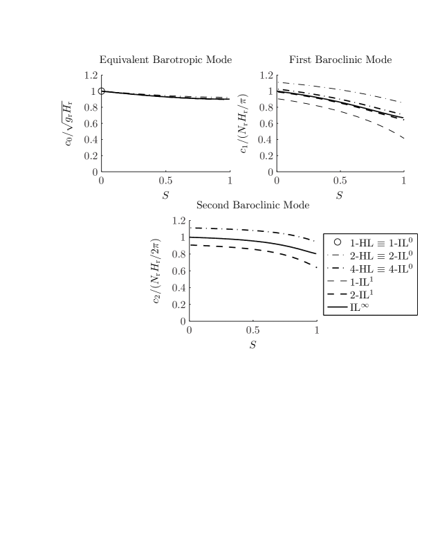
Figure 3: Phase speed of (internal) long gravity waves as a function of the stratification strength in a reduced-gravity reference state with no currents.

Figure 3 compares, as a function of $S$, the phase speed as determined by the IL^∞, $n$-HL, $n$-IL⁰, and $n$-IL¹ for various $n$. The figure shows the results for the external mode ($c_{0}$), and the first ($c_{1}$) and second ($c_{2}$) internal modes. The analytical expression for the IL^∞’s phase speed for an arbitrary mode number can be found in R95; the phase speeds for the layer models are computed numerically. The solutions of the $n$-HL and $n$-IL⁰ coincide because $\bar{\vartheta}_{i}$ is constant for a normal mode in the $n$-IL⁰. These models can only support $n$ vertical normal modes. In contrast, the $n$-IL¹ sustains vertical normal modes up to the $(n+1)$th internal mode.

As noted above, the 1-IL¹ result coincides with that of IL^∞ for the barotropic mode. To approximate well the exact solution, two HL- or IL⁰-like layers are needed. The first internal mode solution is very well approximated using two IL¹-like layers. Four HL-like layers do not provide a similar degree of approximation. The second internal mode solution is reasonably approximated with two IL¹-like layers. The distance between the exact solution and that produced using four HL-like layers is of the same order. However, in every case the $n$-HL (or the $n$-IL⁰) overestimates the exact phase speeds.

3.8 Baroclinic instability

As one further test of the validity of the $n$-IL¹, the problem of baroclinic instability, particularly upper-ocean baroclinic instability, is considered here. (A subset of the results presented here appeared in Beron-Vera et al. [2004].) The behavior in both quasigeostrophic and ageostrophic regimes is explored. The $n$-IL¹ solutions are compared in all cases with the IL^∞ solutions. In some cases comparisons are also made with $n$-HL and $n$-IL⁰ solutions. In the quasigeostrophic regime analytical expressions exist for the IL^∞ solutions. Analytical or semianalytical formulas for the dispersion relations also exist in this regime for the 1-IL¹ and models with one IL⁰-like or two HL-like layers. The rest of the solutions shown are computed numerically upon finite differencing the corresponding eigenvalue problems.

Upper-ocean baroclinic instability, e.g., above the ocean thermocline, is studied in Beron-Vera and Ripa [1997] using the IL^∞ and the 1-IL¹ in a reduced-gravity setting. A basic state with a parallel current $\mathbf{U}=U(z)\,\hat{\mathbf{x}}$ is considered in that work to lie in an infinite channel on the $f$ plane, to have a uniform vertical shear, and to be in thermal-wind balance with the across-channel buoyancy gradient. The basic velocity is further set to vary (linearly) from $\bar{U}+U^{\sigma}$ at the top of the active layer to $\bar{U}-U^{\sigma}$ at the base of the active layer. Accordingly, the basic buoyancy field $\Theta(y,z)$ varies from $g_{\mathrm{r}}(1-2fU^{\sigma}y/H_{\mathrm{r}}+S)$ at the top of the active layer to $g_{\mathrm{r}}(1-2fU^{\sigma}y/H_{\mathrm{r}}-S)$ at the base of the active layer ($y$ is the across-channel coordinate). A nonvanishing velocity at the base of the active layer implies that the latter has a linear $y$-slope given by $g_{\mathrm{r}}^{-1}f\left(U^{\sigma}-\bar{U}\right)/(1-S)$. This basic state is a steady solution of the IL^∞ to the lowest order in the Rossby number, $\mathrm{Ro}:=\bar{U}/L|f|\sim U^{\sigma}/L|f|$ where $L$ is the relevant length scale, which is assumed to be an infinitesimal parameter. In the limit of weak stratification $(S\rightarrow 0)$ the horizontal scales

$$R_{\mathrm{E}}:=\frac{\sqrt{g_{\mathrm{r}}H_{\mathrm{r}}}}{\left|f\right|},\quad R_{\mathrm{I}}:=\frac{N_{\mathrm{r}}H_{\mathrm{r}}}{\left|f\right|}$$ (37)

are well separated $(R_{\mathrm{E}}\gg R_{\mathrm{I}})$, and thus long and short normal-mode perturbations to this state can be identified. Under long small-Rossby-number normal-mode perturbations the base of the active layer behaves as a free boundary. For short small-Rossby-number normal-mode perturbations this interface is effectively rigid. When the vertical shear is assumed strong, $\bar{U}/U^{\sigma}\ll O(S^{-1}),$ the short-perturbation limit corresponds to the classical Eady problem of baroclinic instability, in whose case solutions are insensitive to $\bar{U}/U^{\sigma}$.

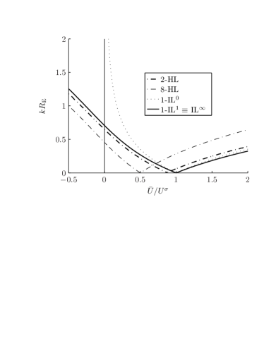
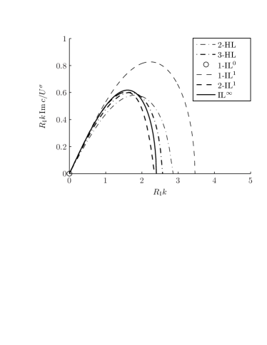
Figure 4: (left panel) Minimum wavenumber for long-perturbation and strong-shear (i.e., free-boundary) baroclinic instability as a function of the slope of the lower interface in the basic state. (right panel) Growth rate of the most unstable perturbation as a function of the wavenumber in short-perturbation, strong-shear (i.e., classical Eady) baroclinic instability.

The left panel of Figure 4 shows the minimum along-channel wavenumber, $k$, for instability as a function of $\bar{U}/U^{\sigma}$ in the long-perturbation and strong-shear limits (free-boundary baroclinic instability). The 1-IL¹ gives the exact result for all $\bar{U}/U^{\sigma}$ [Beron-Vera and Ripa, 1997]. To provide a close approximation to this result for all $\bar{U}/U^{\sigma}$ with the $n$-HL, a fairly large $n$ (cir. $25$) is needed. Note that the 1-IL⁰ predicts, incorrectly, stability for $\bar{U}/U^{\sigma}<0$ (the vertical shear in this model is implicit through the thermal-wind relation).

The right panel of Figure 4 depicts, as a function of the along-channel wavenumber $k$, the growth rate of the most unstable perturbation in the short-perturbation and strong-shear limits (classical baroclinic instability). The comparison of the maximum growth rate predicted by the 1-IL¹ with the IL^∞’s maximum growth rate is less satisfactory in this limit. However, and very importantly, a high wavenumber cutoff of baroclinic instability is present. The 1-IL⁰ model only gives the $k=0$ value of the growth rates of this figure and thus it cannot be used to describe this regime ($N_{\mathrm{r}}\equiv 0$ in this model). Three IL¹-like layers are enough to approximate well the exact maximum growth rate for all $k$. To obtain a similar result using HL-like layers, at least $6$ must be considered.

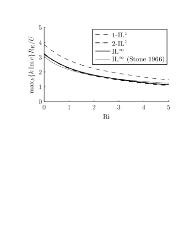
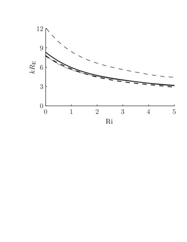
Figure 5: (left panel) Maximum normal-mode perturbation growth rate for ageostrophic (classical Stone) baroclinic instability as a function of the Richardson number. (right panel) Wavenumber for maximum growth rate.

For the basic state considered above the Richardson number

$$\mathrm{Ri}:=\left(\frac{N_{\mathrm{r}}}{\partial_{z}U}\right)^{2}\equiv\frac{SR_{\mathrm{E}}^{2}}{2\mathrm{Ro}^{2}L^{2}}.$$ (38)

In classical baroclinic instability, for which $\mathrm{Ro},S\rightarrow 0$, $L=R_{\mathrm{I}}\equiv\sqrt{2S}R_{\mathrm{E}}$ and $\bar{U}/U^{\sigma}\ll O(S^{-1}),$ the well-known result $\mathrm{Ri}\rightarrow\infty$ holds. In free-boundary baroclinic instability, for which $\mathrm{Ro},S\rightarrow 0$, $L=R_{\mathrm{E}}$ and $\bar{U}/U^{\sigma}\ll O(S^{-1}),$ $\mathrm{Ri}$ can acquire any value because a proper way [Beron-Vera and Ripa, 1997] to achieve the $S\rightarrow 0$ limit is to set $S=O(\mathrm{Ro}^{\nu})$ for any $\nu$. Unlike quasigeostrophic baroclinic instability, ageostrophic baroclinic instability is characterized by a dependence of the solutions on $\mathrm{Ri}$ [Stone, 1966; 1970]. This dependence is checked in the present layer model by considering infinitesimal nongeostrophic normal-mode perturbations to the above basic state but with $\bar{U}\equiv U^{\sigma}=U$, and assuming $\mathrm{Ro}=10^{-1}$ and $L=R_{\mathrm{E}}$.

The left panel of Figure 5 shows, as a function of $\mathrm{Ri}$, the maximum growth rate $\max_{k}\{k\operatorname{Im}c\}$ of the perturbation. The right panel of the figure shows, also as a function of $\mathrm{Ri}$, the wavenumber, $k_{\max}$, at which the latter value is attained. Shown for reference is an IL^∞ asymptotic solution, valid up to $O(\mathrm{Ro}^{3})$. The asymptotic formulas for $\max_{k}\{\operatorname{Im}kc\}$ and $k_{\max}$ are those given in equations (4.27) and (4.28) of Stone [1966]. The $n$-IL¹ fares very well even with $n=1$. A model with a single IL⁰-like layer, however, cannot describe this regime because of the dependence on $\mathrm{Ri}$ (for the 1-IL⁰ $S\equiv 0$). With two IL¹-like layers the maximum growth rates and corresponding wavenumbers at which they are achieved are in very close agreement with the IL^∞ predictions in the range of $\mathrm{Ri}$ values explored, which was much wider than that shown in Figure 5. Note, however, that observations indicate that typical values of $\mathrm{Ri}$ in the upper ocean are close to unity [e.g., Tandon and Garrett, 1994]

3.9 Forcing

In R95 forcing (wind stress, interfacial drag, and buoyancy/heat input) was introduced in the $1$-IL¹ model equations in a way that was compatible with the conservation laws of energy, momentum, and mass/heat content. The same approach is adopted here to include, in addition, freshwater fluxes through the surface in accordance with the conservation law of salt content. The possibility for the exchange of fluid across the other interfaces is also considered.

Let $\mathbf{\tau}(\mathbf{x},t)$ be a wind stress acting at the surface of the ocean ($\rho_{n+1}\equiv 0$ must be the setting in the rigid-bottom configuration and typically $h_{0}\equiv 0$ in the rigid-lid one). Assume further that there is a friction force acting at the interface between contiguous layers. Introduction of these forces in Newton’s equations (12d,e) in the form

$$\partial_{t}\mathbf{\bar{u}}_{i}+\cdots =\delta_{i\alpha}\mathbf{\tau}/h_{\alpha}-r_{i}(\mathbf{\bar{u}}_{i}\pm\mathbf{u}_{i}^{\sigma}),$$ (39a)

$$\partial_{t}\mathbf{u}_{i}^{\sigma}+\cdots =\mp 3\delta_{i\alpha}\mathbf{\tau}/h_{\alpha}+3r_{i}(\mathbf{\bar{u}}_{i}\pm\mathbf{u}_{i}^{\sigma}),$$ (39b)

implies that the work done by the wind stress is proportional to the velocity at the top of the uppermost layer, $\mathbf{\bar{u}}_{\alpha}\mp\mathbf{u}_{\alpha}^{\sigma}$, and that one done by the friction force in the $i$th layer is proportional to the velocity at the base of that layer, $\mathbf{\bar{u}}_{i}\pm\mathbf{u}_{i}^{\sigma}$. Namely,

$$\partial_{t}\sum_{j}E_{j}+\cdots =\mathbf{\tau}\cdot(\mathbf{\bar{u}}_{\alpha}\mp\mathbf{u}_{\alpha}^{\sigma})-\sum_{j}r_{j}h_{j}(\mathbf{\bar{u}}_{j}\pm\mathbf{u}_{j}^{\sigma})^{2},$$ (40a)

$$\partial_{t}\sum_{j}M_{j}+\cdots =\mathbf{\tau}\cdot\mathbf{\hat{x}}-\sum_{j}r_{j}h_{j}(\mathbf{\bar{u}}_{j}\pm\mathbf{u}_{j}^{\sigma})\cdot\mathbf{\hat{x}}.$$ (40b)

In the above equations, $\delta_{ij}$ is the Kroenecker delta and $r_{i}$ is a friction coefficient that can be taken as a constant or as some function of $h_{i}$ and $|\mathbf{\bar{u}}_{i}\pm\mathbf{u}_{i}^{\sigma}|.$ [Recall that $\alpha:=n$ (resp., $\alpha:=1$) for the rigid-bottom (resp., rigid-lid) configuration.]

Let now $\Gamma(\mathbf{x},t)$ be a buoyancy input through the surface and write the buoyancy equations (12a,b) in the form

$$\partial_{t}\bar{\vartheta}_{i}+\cdots =\delta_{i\alpha}\Gamma/h_{\alpha},$$ (41a)

$$\partial_{t}\vartheta_{i}^{\sigma}+\cdots =\eta\delta_{i\alpha}\Gamma/h_{\alpha},$$ (41b)

where $$\eta$$ is any constant. Consider, in addition, the possibility of fluid crossing the interface between consecutive layers; then the volume conservation equation (12c) can be rewritten as

$$\partial_{t}h_{i}+\cdots=w_{i}^{\mathrm{b}}-w_{i}^{\mathrm{t}}.$$ (41c)

Here, the quantities $w_{i}^{\mathrm{t}}(\mathbf{x},t)$ and $w_{i}^{\mathrm{b}}(\mathbf{x},t)$ are volume fluxes per unit area through the top and base of the $i$th layer, respectively. The set (41), for any value of $\eta$, is compatible with the mass conservation equation

$$\partial_{t}(h_{i}\bar{\vartheta}_{i})+\cdots=\delta_{i\alpha}\Gamma+\bar{\vartheta}_{i}(w_{i}^{\mathrm{b}}-w_{i}^{\mathrm{t}}).$$ (42)

At the surface $w_{\alpha}^{\mathrm{t}}(\mathbf{x},t)=E(\mathbf{x},t)-P(\mathbf{x},t),$ which represents the imbalance of evaporation minus precipitation. Away from the surface some parametrization must be adopted. In models with IL⁰-like layers it is commonly set [e.g., McCreary et al., 1991]

$$w_{i}^{\mathrm{b}}-w_{i}^{\mathrm{t}}=(-1)^{i+1}\dfrac{(h_{i-1}-H_{i-1}^{\mathrm{e}})^{2}}{H_{i-1}^{\mathrm{e}}t_{i}^{\mathrm{e}}}\theta(H_{i-1}^{\mathrm{e}}-h_{i-i}).$$ (43)

Here, $H_{i}^{\mathrm{e}}$ and $t_{i}^{\mathrm{e}}$ are constants that with units of length and time, respectively, that characterize the “entrainment” process, and $\theta(\cdot)$ is the Heaviside step function. In the present case, an algorithm may be designed such that condition (9) is fulfilled at all times. This would allow for a more natural representation of mixing processes, including the possibility of representing localized mixing events, e.g., characterized by $\bar{\vartheta}_{i+1}+\vartheta_{i+1}^{\sigma}<\bar{\vartheta}_{i}-\vartheta_{i}^{\sigma}$ instantaneously at certain position. This subject deserves to be studied in detail.

Let finally assume a linear state equation, i.e., $\vartheta_{i}=g\alpha_{T}(T_{i}-T_{n+1})-g\alpha_{S}(S_{i}-S_{n+1}).$ Here, $\alpha_{T}$ and $\alpha_{S}$ are the thermal expansion and salt contraction coefficients, respectively; $T_{i}(\mathbf{x},\sigma,t)=\bar{T}_{i}(\mathbf{x},t)+\sigma T_{i}^{\sigma}(\mathbf{x},t)$ and $S_{i}(\mathbf{x},\sigma,t)=\bar{S}_{i}(\mathbf{x},t)+\sigma S_{i}^{\sigma}(\mathbf{x},t)$ are the $i$th layer temperature and salinity, respectively; and $T_{n+1}$ and $S_{n+1}$ are the inactive layer (constant) temperature and salinity, respectively. Let also write the buoyancy input as

$$\Gamma=g\alpha_{T}(\rho_{\mathrm{r}}C_{p})^{-1}Q+g\alpha_{S}\bar{S}_{\alpha}(P-E),$$ (44)

$C_{p}$ is the specific heat at constant pressure and $Q(\mathbf{x},t)$ is the heat input through the surface. Equation (42) can then be split into a heat and salt content conservation equations, namely,

$$\partial_{t}(h_{i}\bar{T}_{i})+\cdots =\delta_{i\alpha}(\rho_{\mathrm{r}}C_{p})^{-1}Q+\bar{T}_{i}(w_{i}^{\mathrm{b}}-w_{i}^{\mathrm{t}}),$$ (45a)

$$\partial_{t}(h_{i}\bar{S}_{i})+\cdots =\delta_{i\alpha}\bar{S}_{\alpha}(E-P)+\bar{S}_{i}(w_{i}^{\mathrm{b}}-w_{i}^{\mathrm{t}}).$$ (45b)

If fluid across the surface is allowed only, the choice (44) enforces, on one hand [e.g., Beron-Vera et al., 1999],

$$\frac{\mathrm{d}}{\mathrm{d}t}\int_{j}h_{j}\bar{S}_{j}\equiv 0,$$ (46a)

and, on the other [Beron-Vera and Ripa, 2000],

$$\frac{\mathrm{d}}{\mathrm{d}t}\left\langle T\right\rangle=V^{-1}\int_{D}(\rho_{\mathrm{r}}C_{p})^{-1}Q\operatorname{d}\!{}^{2}\mathbf{x}+(\bar{T}_{\alpha}-\left\langle T\right\rangle)(P-E),$$ (46b)

where $V:=\int_{j}h_{j}\equiv\int_{D}\mathrm{d}^{2}\mathbf{x}$ $h$ is the total volume and $\left\langle T\right\rangle:=V^{-1}\int_{j}h_{j}\bar{T}_{j}$ is the average temperature in $V$. Note that (46b), unlike the equation satisfied by $\int_{j}h_{j}\bar{T}_{j},$ is independent—as it should—of the choice of the origin of the temperature scale [cf. Warren, 1999].

4 Concluding remarks

This paper describes a multilayer extension of the single-layer primitive-equation model for ocean dynamics and thermodynamics introduced in Ripa [1995]. Inside each layer the velocity and buoyancy fields can vary not only arbitrarily in the horizontal position and time, but also linearly with depth.

In the absence of external forcing and dissipation, the model conserves volume, mass, buoyancy variance, energy, and zonal momentum for zonally symmetric horizontal domains and topographies. Unlike models with depth-independent velocity and buoyancy fields within each layer, the model generalized here is able to represent the thermal wind balance explicitly at low frequency inside each layer. In this sense, the model of this paper has “better” physics than a model with depth-independent fields. For a fixed number of layers, the model of this paper can sustain one more vertical normal mode than the homogeneous-layer models, which, on the other hand, are not able to incorporate thermodynamic processes (e.g., due to heat and buoyancy fluxes across the air–sea interface or associated with localized vertical mixing events). In this other sense, the present model has “more” physics than a model with homogeneous layers. Last but not least, overall improved results in both quasigeostrophic (free-boundary and classical Eady) and ageostrophic (classical Stone) baroclinic instability with respect to the single-layer calculations are attained with the addition of a small number layers.

The present generalization enriches Ripa’s single-layer model by providing it enough flexibility to approach problems for which a single-layer structure is too idealized. Configurations with a small number of layers are particularly useful for the insight they provide into physical processes. Configurations with more layers may provide the basis for an accurate numerical circulation model.

Finally, and returning to the motivation for revisiting the construction of models with reduced thermodynamics, the requirement on the two-dimensional structure of the models is satisfied by the model derived here. A different strategy than that taken here is needed to fulfill the requirement on the geometric structure of the models, if the goal is to pursue flow-topology-preserving parameterizations of unresolved scales using the SALT (stochastic advection by Lie transport) framework [Holm, 2015; Holm and Luesink, 2020]. The desired result might follow from plugging Ripa’s ansatz in the Hamilton principle’s Lagrangian of the primitive equations for continuously stratified fluid. This is currently under investigation. A stochastic parameterization framework that can be applied to the model derived here is location uncertainty (LU) [Resseguier et al., 2020]. Unlike SALT dynamics, which preserve Kelvin circulation, the LU framework conserves energy, so it can be immediately applied on the present model and is a natural fit to considering the parameterizations based on extraction of available potential energy [Gent and Mcwilliams, 1990; Fox-Kemper et al., 2008; Bachman et al., 2017]. Building stochastic parameterizations using the generalized Ripa’s model is left for future work.

Acknowledgements.

A stimulating epistolary exchange with Darryl Holm provided incentive to revisit this work and finish it.

References

- Abarbanel et al. [1986] Abarbanel H., Holm D., Marsden J., and Ratiu T. [1986]. Philos. Trans. R. Soc. London, A 318, 349–409.
- Anderson and McCreary [1985] Anderson D. L. T., and McCreary J. P. [1985]. J. Atmos. Sci. 42, 615–629.
- Arnold [1965] Arnold V. I. [1965]. Dokl. Akad. Nauk. SSSR 162, 975–978, engl. transl. Sov. Math. 6: 773-777 (1965).
- Arnold [1966] Arnold V. I. [1966]. Izv. Vyssh. Uchebn. Zaved Mat. 54, 3–5, engl. transl. Am. Math. Soc. Transl. Ser. 2 79: 267-269 (1969).
- Bachman et al. [2017] Bachman S., Fox-Kemper B., Taylor J., and Thomas L. [2017]. Ocean Modelling 109, 72 – 95.
- Beier [1997] Beier E. [1997]. J. Phys. Oceanogr. 27, 615–632.
- Beier and Ripa [1999] Beier E., and Ripa P. [1999]. J. Phys. Oceanogr. 29, 305–311.
- Benilov [1993] Benilov E. [1993]. J. Fluid Mech. 251, 501–514.
- Beron-Vera et al. [1999] Beron-Vera F. J., Ochoa J., and Ripa P. [1999]. Ocean Modell. 1, 111–118.
- Beron-Vera et al. [2004] Beron-Vera F. J., Olascoaga M. J., and Zavala-Garay J. [2004]. In ICTAM04 Abstract Book and CD-ROM Proceedings. ISBN 83-89687-01-1, IPPT PAN, Warsaw.
- Beron-Vera and Ripa [1997] Beron-Vera F. J., and Ripa P. [1997]. J. Fluid Mech. 352, 245–264.
- Beron-Vera and Ripa [2000] Beron-Vera F. J., and Ripa P. [2000]. J. Geophys. Res. 105, 11441–11457.
- Beron-Vera and Ripa [2002] Beron-Vera F. J., and Ripa P. [2002]. J. Geophys. Res. 107 (C8), 10.1029/2000JC000769.
- Boccaletti et al. [2007] Boccaletti G., Ferrari R., and Fox-Kemper B. [2007]. J. Phys. Oceanogr. 37, 2228–2250.
- Britton and Xing [2020] Britton J., and Xing Y. [2020]. Journal of Scientific Computing 82, 2.
- Bröcker et al. [2018] Bröcker J., et al. [2018]. Mathematics of Planet Earth: A Primer. World Scientific.
- Cotter et al. [2020] Cotter C., Crisan D., Holm D., Pan W., and Shevchenko I. [2020]. J. Stat. Phys. 179, 1186 – 1221.
- Dellar [2003] Dellar P. J. [2003]. Phys. Fluids 15, 292–297.
- Desveaux et al. [2015] Desveaux V., Zenk M., Berthon C., and Klingenberg C. [2015]. Mathematics of Computation 85, 1.
- Dronkers [1969] Dronkers J. [1969]. J. Hydrau. Div. 95, 44–77.
- Fox-Kemper et al. [2008] Fox-Kemper B., Ferrari R., and Hallberg R. [2008]. Journal of Physical Oceanography 38, 1145–1165.
- Fukamachi et al. [1995] Fukamachi Y., McCreary J. P., and Proehl J. A. [1995]. J. Geophys. Res. 100, 2559–2577.
- Gent and Mcwilliams [1990] Gent P. R., and Mcwilliams J. C. [1990]. Journal of Physical Oceanography 20, 150–155.
- Gouzien et al. [2017] Gouzien E., Lahaye N., Zeitlin V., and Dubos T. [2017]. Physics of Fluids 29, 101702.
- Haine and Marshall [1998] Haine T. W., and Marshall J. [1998]. J. Phys. Oceanogr. 28, 634–658.
- Holm et al. [1983] Holm D., Marsden J., Ratiu T., and Weinstein A. [1983]. Phys. Lett. A 98, 15–21.
- Holm [1996] Holm D. D. [1996]. Physica D 98, 379–414.
- Holm [2015] Holm D. D. [2015]. Proceedings of the Royal Society A: Mathematical, Physical and Engineering Sciences 471, 20140963.
- Holm and Luesink [2020] Holm D. D., and Luesink E. [2020]. arXiv:1910.10627.
- Holm et al. [2020] Holm D. D., Luesink E., and Pan W. [2020]. arXiv:2006.05707.
- Holm et al. [2002] Holm D. D., Marsden J. E., and Ratiu T. S. [2002]. In Large-Scale Atmosphere-Ocean Dynamics II: Geometric Methods and Models (ed. J. Norbury and I. Roulstone), pp. 251–299. Cambridge University.
- Lahaye et al. [2020] Lahaye N., Zeitlin V., and Dubos T. [2020]. Ocean Modelling 153, 101673.
- Lavoie [1972] Lavoie R. [1972]. J. Atmos. Sci. 29, 1025 – 1040.
- McCreary et al. [1991] McCreary J. P., Fukamachi Y., and Kundu P. [1991]. J. Geophys. Res. 96, 2515–2534.
- McCreary et al. [2001] McCreary J. P., et al. [2001]. J. Geophys. Res. 106, 7139–7155.
- McCreary and Kundu [1988] McCreary J. P., and Kundu P. [1988]. J. Mar. Res. 46, 25–58.
- McCreary et al. [1997] McCreary J. P., Zhang S., and Shetye S. R. [1997]. J. Geophys. Res. 102, 15,535–15,554.
- McIntyre and Shepherd [1987] McIntyre M., and Shepherd T. [1987]. J. Fluid Mech. 181, 527–565.
- McWilliams [2016] McWilliams J. C. [2016]. Proc R Soc A 472, 20160117.
- Morrison [1982] Morrison P. J. [1982]. In Mathematical Methods in Hydrodynamics and Integrability in Dynamical Systems (ed. M. Tabor and Y. Treve), pp. 13–46. Institute of Physics Conference Proceedings 88.
- Mungkasi and Roberts [2016] Mungkasi S., and Roberts S. G. [2016]. J. Phys.: Conf. Ser. 693, 012011.
- O’Brien and Reid [1967] O’Brien J. J., and Reid R. O. [1967]. J. Atmos. Sci. 24, 197–207.
- Ochoa et al. [1998] Ochoa J. L., Sheinbaum J., and Pavía E. G. [1998]. J. Geophys. Res. 103, 24869–24880.
- Palacios-Hernández et al. [2002] Palacios-Hernández E., Beier E., Lavín M. F., and Ripa P. [2002]. J. Phys. Oceanogr. 32, 705–728.
- Pedlosky [1987] Pedlosky J. [1987]. Geophysical Fluid Dynamics, 2nd edn. Springer.
- Pinet and Pavía [2000] Pinet R., and Pavía E. [2000]. J. Fluid Mech. 416, 29–43.
- Rehman et al. [2018] Rehman A., Ali I., and Qamar S. [2018]. Results in Physics 8, 104 – 113.
- Resseguier et al. [2020] Resseguier V., Pan W., and Fox-Kemper B. [2020]. Nonlinear Processes in Geophysics 27, 209–234.
- Ripa [1993] Ripa P. [1993]. Geophys. Astrophys. Fluid Dyn. 70, 85–111.
- Ripa [1994] Ripa P. [1994]. In Modelling of Oceanic Vortices (ed. G. V. Heist), pp. 151–159.
- Ripa [1995] Ripa P. [1995]. J. Fluid Mech. 303, 169–201.
- Ripa [1996a] Ripa P. [1996a]. J. Geophys. Res. C 101, 1233–1245.
- Ripa [1996b] Ripa P. [1996b]. Rev. Mex. Fís. 42, 117–135.
- Ripa [1997] Ripa P. [1997]. J. Phys. Oceanogr. 27, 597–614.
- Ripa [1999] Ripa P. [1999]. Dyn. Atmos. Oceans 29, 1–40.
- Ripa [2001] Ripa P. [2001]. In Proceedings of the 13th Conference on Atmospheric and Oceanic Fluid Dynamics, pp. 1–4. American Meteorological Society.
- Ripa [2003] Ripa P. [2003]. In Nonlinear Processes in Geophysical Fluid Dynamics: A Tribute to the Scientific Work of Pedro Ripa (ed. O. U. Velasco-Fuentes, J. Ochoa and J. Sheinbaum), pp. 103–126. Kluwer. Plublished post mortem.
- Salmon [2004] Salmon R. [2004]. J. Atmos. Sci. 61, 2,016–2,036.
- Sanchez-Linares et al. [2016] Sanchez-Linares C., de Luna T. M., and Castro Diaz M. J. [2016]. Applied Mathematics and Computation 272, 369–384.
- Schopf and Cane [1983] Schopf P., and Cane M. [1983]. J. Phys. Oceanogr. 13, 917–935.
- Scott and Willmott [2002] Scott R. B., and Willmott A. J. [2002]. Dyn. Atmos. Oce. 35, 389–419.
- Shepherd [1990] Shepherd T. G. [1990]. Adv. Geophys. 32, 287–338.
- Stone [1966] Stone P. H. [1966]. J. Atmos. Sci. 23, 390–400.
- Stone [1970] Stone P. H. [1970]. J. Atmos. Sci. 27, 721–726.
- Tandon and Garrett [1994] Tandon A., and Garrett C. [1994]. J. Phys. Oceanogr. 24, 1419–1424.
- Warnerford and Dellar [2013] Warnerford E. S., and Dellar P. J. [2013]. J. Fluid Mech. 723, 374–403.
- Warren [1999] Warren B. A. [1999]. J. Geophys. Sci. 104, 7915–7919.
- Young [1994] Young W. R. [1994]. J. Phys. Oceanogr. 24, 1812–1826.
- Young and Chen [1995] Young W. R., and Chen L. [1995]. J. Phys. Oceanogr. 25, 3172–3185.
- Zavala-Hidalgo et al. [2002] Zavala-Hidalgo, J. J., Pares-Sierra A., and Ochoa J. [2002]. Atmosfera 15, 81 – 104.
- Zeitlin [2018] Zeitlin V. [2018]. Geophysical fluid dynamics: understanding (almost) everything with rotating shallow water models. Oxford University Press.