Start-to-End Simulations of SASE FEL at the TESLA Test Facility, Phase 1

Abstract

Phase 1 of the vacuum ultra-violet (VUV) free-electron laser (FEL) at the TESLA Test Facility (TTF) recently concluded operation. It successfully demonstrated the saturation of a SASE FEL in the in the wavelength range of 80-120 nm. We present a posteriori  start-to-end numerical simulations of this FEL. These simulations are based on the programs Astra and elegant for the generation and transport of the electron distribution. An independent simulation of the intricate beam dynamics in the magnetic bunch compressor is performed with the program CSRtrack. The SASE FEL process is simulated with the code FAST. From our detailed simulations and the resulting phase space distribution at the undulator entrance, we found that the FEL was driven only by a small fraction (slice) of the electron bunch. This “lasing slice” is located in the head of the bunch, and has a peak current of approximately 3 kA. A strong energy chirp (due to the space charge field after compression) within this slice had a significant influence on the FEL operation. Our study shows that the radiation pulse duration is about 40 fs (FWHM) with a corresponding peak power of 1.5 GW. The simulated FEL properties are compared with various experimental data and found to be in excellent agreement.

DESY 03-197

December 2003

, , , , , , and

1 Introduction

The vacuum ultra-violet (VUV) free-electron laser (FEL) at the TESLA Test Facility (TTF), Phase 1 demonstrated saturation in the wavelength range 80-120 nm based on the self-amplified spontaneous emission (SASE) principle[1, 2, 3]. Analysis of experimental data for the radiation properties have led us to the unique conclusion that SASE FEL produced ultra-short radiation pulse (FWHM duration 30-100 fs) with GW level of peak power. However the measured properties of the radiation were in strong disagreement with project parameters for the electron bunch [4]: we expected a peak beam current of 500 A, an rms bunch duration of 1 ps, and an energy spread of 0.5 MeV. Such electron beam parameters would result in operation of the FEL in the saturation regime only for normalized emittance less or about 2 mm-mrad, while emittance measurements gave values of approximately 4 mm-mrad for a bunch charge of 1 nC [5]. Also, the radiation pulse was by one order of magnitude shorter than the value expected for the aforementioned project parameters.

Facing this evident disagreement, we did an attempt to reconstruct parameters of the lasing part of the electron bunch using measured properties of the radiation[1, 2, 3]. Actually, radiation measurements were very reliable and accurate, and in combination with the FEL theory we can infer a lot about the properties of the part of electron bunch that produces the radiation. In the FEL simulations[1, 2, 3] lasing part of the bunch was approximated by a Gaussian. A set of parameters for this lasing part of the electron bunch leading to simulation results, consistent with the radiation measurements, were: a FWHM bunch duration of 120 fs, a peak current of 1.3 kA, an rms energy spread of 100 keV, and a rms normalized transverse emittance of 6 mm-mrad. These values, as used in the FEL-simulation, gave reasonable agreement for the average energy in the radiation pulse and statistical distributions of the fluctuations of the radiation energy. However, there were two visible disagreements with experimentally measured radiation characteristics. First, there was a noticeable difference in the shape of angular distribution of the radiation intensity. Second, the measured averaged spectrum width was visibly wider with respect to the simulated one and the spikes in the single-shot spectra were larger in the experiment than the one simulated.

It is worth mentioning that soon after obtaining the saturation, attempts for more detailed electron beam measurements were undertaken. The first one was measurement of the slice energy spread before compression [6] which gave the value of about 5 keV. This measurement clearly indicated that the value of peak current after compression should be well above 1.3 kA. The second experiment aimed at direct time-domain measurement with a streak camera [5] of the bunch shape and peak current. The results of these measurements gave $650\pm 100$ fs for rms pulse duration, and 0.6 kA peak current at 3 nC. These results were consistent with another techniques based on a tomographic reconstruction of the longitudinal phase space[8]. Both of these measurement were in fact resolution limited: for instance the temporal resolution of the streak camera in the experiment reported in [5] was 200 fs. It was therefore impossible to resolve any fine structure on the bunch charge density that have characteristic width below $\sim$200 fs. Hence it was impossible to resolve the lasing fraction of the bunch since it was below 200 fs as we mentioned above. We should also note that there was no possibility to measure slice emittance and energy spread at TTF.

Thus there was no complete quantitative description of the TTF SASE FEL operation. To get a better understanding of the TTF SASE FEL operation we undertook the full physics simulation of the TTF FEL, Phase 1. This study aimed to trace the evolution of the electron beam from the photo-cathode to the undulator entrance. Then use the thereby produced electron distribution to calculate the radiation produced by this electron bunch while passing in the undulator. In our simulations we tried (to our best knowledge) to reproduce the main parameters of the machine from the FEL run in September 2001. In some cases, due to the lack of reliable informations, we had to make simplified assumptions.

Presently there is no universal particle tracking code capable of the evolution of the electron beam through the accelerator and bunch compression chain. For the simulation reported hereafter, the program ASTRA [9], which takes into account space charge, but does not calculate the beam dynamics in the bends, was used in straight transport sections (gun, capture cavity, accelerating modules, drift spaces). The beam dynamics in the bunch compressor was independently simulated with the codes elegant [10] and CSRtrack [11] taking into account the effects related to coherent synchrotron radiation (CSR). Finally, the FEL process was simulated by three-dimensional, time-dependent code FAST [12].

2 Facility description

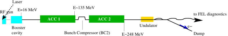
Figure 1: Schematic layout of the TESLA Test Facility, Phase 1

The description of the TTF accelerator (see Fig. 1), operating under standard lasing conditions, can be found in[2, 3] and references therein. The RF gun consists of an L-band cavity (1+1/2 cell) incorporating a CsTe₂ photo-cathode illuminated by a UV laser with a (Gaussian) pulse distribution of 7-8 ps rms. The electron bunch with the charge 2.8 nC and energy about 4 MeV is extracted from the gun (nominal laser launch phase is 40 deg) and is then accelerated in the booster cavity up to 16 MeV. The phase of the booster cavity is normally chosen such that the total (correlated) energy spread is minimized. Passing a rather long drift, the beam is then injected into the superconducting TESLA module (ACC1) where it is accelerated up to 135 MeV off-crest to impart the proper correlated energy spread for subsequent compression in the following four-bend magnetic chicane (BC2). Without compression the bunch is rather long (about 3.5 mm rms - longer than the laser pulse due to Coulomb repulsing in the injector). Thus, at the nominal compression phase (10 deg off-crest) the bunch accumulates RF curvature leading to a ”banana” shape on the longitudinal phase plane after compression. The resulting bunch shape in time domain constitutes a short high-current leading peak and a low-current long tail. After compression the beam passes a 5 m long drift, the second TESLA module ACC2 (being accelerated up to 248 MeV), and another drift (about 20 m) that includes a collimation section and a transverse matching section. Finally the beam enters the undulator consisting of three 4.5 m long modules where a short SASE pulse (wavelength below 100 nm) is produced by the leading peak of the bunch. The electron beam is separated from the photon beam thanks to the spectrometer dipole, and bent in a beam dump while the photon beam goes to the photon diagnostic area.

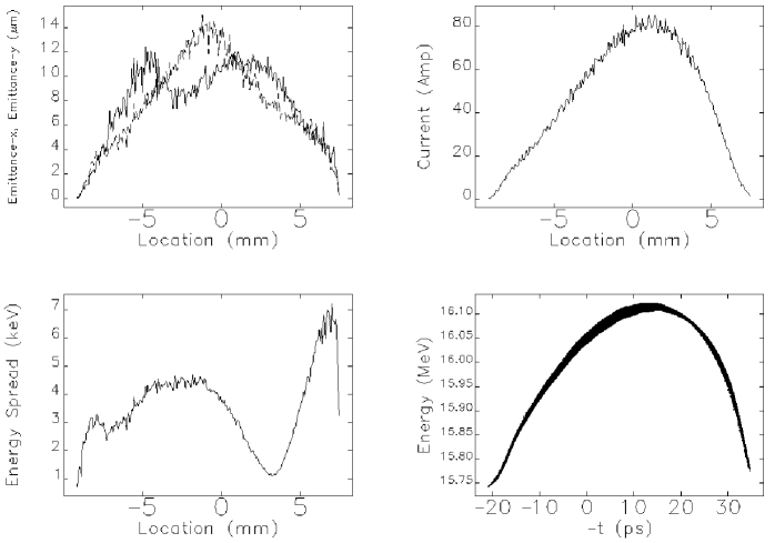
Figure 2: Normalized slice emittance (x - line, y - dash), current, slice energy spread, and longitudinal phase plane at the entrance to ACC1. Bunch head is on the right

3 Simulations of the beam dynamics in the accelerator

The initial part of the accelerator, from the photo-cathode to BC2 entrance, was simulated with Astra [9], a program that includes space charge field using a cylindrical symmetric grid algorithm. The beam was then tracked through the bunch compressor with elegant [10] that includes a simplified model (based on a line charge approximation) of the CSR wake[13, 14]. Downstream of BC2, Astra was again used up to the undulator entrance because the space charge induced-effects are significant for the strongly compressed part of the bunch. SASE FEL process in the undulator was simulated with three-dimensional time-dependent code FAST [12]. In order to check that we did not miss any important CSR-related effects in the bunch compressor, we performed an independent simulations of the bunch compressor with a newly developed code CSRtrack [11]. This latter code incorporates a two-dimensional self-consistent model of the beam dynamics.

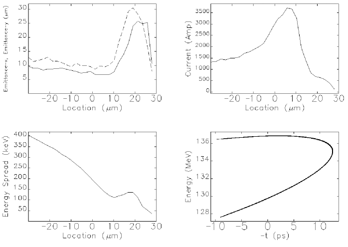
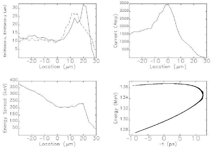
Figure 3: Normalized slice emittance (x - line, y - dash), current, slice energy spread in the front part of the bunch, and longitudinal phase plane. The position is behind the bunch compressor. CSR is off. Bunch head is on the right

Figure 4: Normalized slice emittance (x - line, y - dash), current, slice energy spread in the front part of the bunch, and longitudinal phase plane. CSR is on. The position is behind the bunch compressor. Bunch head is on the right

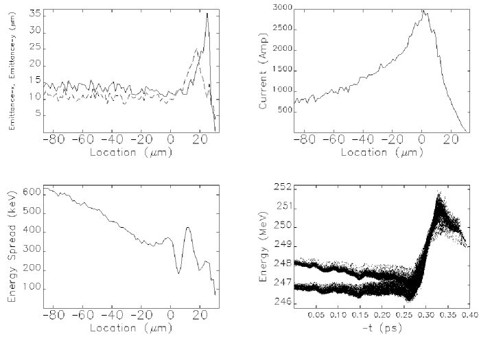
Figure 5: Normalized slice emittance (x - line, y - dash), current, slice energy spread, and longitudinal phase plane for the front part of the bunch. The position is at the undulator entrance. Bunch head is on the right

The Astra simulation from the cathode to the bunch compressor was performed using $2\times 10^{5}$ macro-particles. The main parameters of the electron beam, calculated for various longitudinal slices along the bunch, at the entrance to ACC1 are presented in Fig. 2. The chosen bin size is such that the energy chirp does not contribute to the slice energy spread. The latter parameter is very important since it defines the width of the leading peak and the peak current after compression. One can see that it varies along the bunch, taking the value of about 3.5 keV at the location $s=0$ (this part of the bunch is then put into a local full compression in BC2). The resulting values for the local energy spread in Fig. 2 are in agreement with the measurements [6]. The main source of the build-up of the local energy spread (as we see it from this simulation) is a transverse variation of the longitudinal space charge field in the injector. Since it is a coherent effect (a particle’s energy deviation is correlated with its position in the bunch, in particular, with its transverse offset within a given slice), the frequently used notions of ”uncorrelated” or ”incoherent” energy spread are not adequate here. As we will see, the correlations can be important when we compress the beam.

At the entrance of BC2 the output distribution of macro-particles is converted into the input distribution for elegant. It is then tracked through the bunch compressor ($R_{56}\simeq 23$ cm) without CSR wake included. The resulting distribution on longitudinal phase plane and slice parameters for the leading peak are presented in Fig. 4. One can see that the peak current and the width of the current spike are in a reasonable agreement with analytical estimate, presented in Appendix. The difference can be explained by the non-Gaussian energy distribution in a slice before compression and by the fact that the beam entered ACC1 with the energy 16 MeV and some energy chirp, etc. Also, important correlations in particle distribution are not considered in Appendix. What requires some explanations is a behavior of the slice emittance in Fig. 4. As we have already mentioned, the main effect, responsible for a slice energy spread in the injector, is the transverse variation of the longitudinal space charge field. An energy offset of a particle in a slice (with respect to on-axis particle) is correlated with its transverse offset (and, since particles are moving transversely, with a betatron amplitude). A sign of the energy offset depends on the position of the slice in the bunch. Indeed, the head of the bunch is accelerated due to space charge field, so that for a given slice a particle with a finite betatron amplitude gets less energy than an on-axis particle. The situation is opposite for the slices which are on the left from a minimum energy spread in Fig. 2: the larger transverse offset, the larger positive energy deviation. During compression particles with higher energies (in our case, with larger betatron amplitudes) move forward, this explains the large slice emittance values for the slices in the leading front of the spike. On the other hand, due to this effect a slice with the maximal current has less ”bad” particles, so that the emittance there is visibly less than that at $\mathrm{s}\simeq 0$ in Fig. 2. We also tried to put the head of the bunch (say $\mathrm{s}\simeq 5$  mm in Fig. 2) into a local full compression. The result was that after compression emittance was smoothly decreasing in the leading front of the spike. It is worth noting that when we prepared a 6-D Gaussian bunch with no correlations (at the entrance to ACC1) and track it through BC2, the slice emittance after compression was the same in all slices and was equal to its value before compression.

Our next step was to track the same particle distribution through the bunch compressor, taking into account CSR wake in a simplified model used in elegant. The beam parameters behind BC2 are presented in Fig. 4. Note that due to CSR-induced effects the peak current slightly decreased, by less than 10%. Slice emittance (in horizontal plane) in the slice with maximal current increased by some 50%, and the local energy spread by almost a factor of 2.

It looks surprising that the peak current is almost unchanged in the presence of the CSR wake. Indeed without including CSR, the final shape of the bunch forms in the end of the third - begin of the fourth dipole of BC2. If one does a naive estimate for the energy kicks due to CSR (on the way to the end of the fourth dipole) for such a narrow peak with so high current, and applies $R_{56}$ to the end of compressor, then one finds out that the distribution of current should be strongly disturbed. The reason why this does not happen can be explained as follows. For our range of parameters, one can not neglect coupling between transverse and longitudinal phase spaces in the bunch compressor (the importance of this effect was pointed out in studies of CSR microbunching instability [16, 17, 18]), described by linear transfer matrix elements $R_{51}$ and $R_{52}$ (the net effect through the whole compressor is zero to first order, and higher order terms are negligible). This coupling makes the leading peak effectively much longer and the current much lower than in the case of zero emittance (the spike gets cleaned up only at the very end of the fourth dipole). Thus, the energy kicks due to CSR are strongly suppressed, and the current spike survives.

In order to confirm this result and to check that we did not miss any important effect, using a simplified CSR model in elegant, we performed alternative simulations for the bunch compressor with the ”first principles” code CSRtrack. For technical reasons, the incoming distribution of macro-particles has to be simplified in those simulations (for instance, the above mentioned correlations were neglected), so that slice parameters after compression are not exactly reproduced even without CSR. Nevertheless, the main results of simulations with elegant were confirmed: the peak current decreases by less than 10%, and the slice emittance growth is in the range of several tens of per cent.

¿From BC2 exit to the undulator entrance the tracking was done with Astra. The reason is that a simple estimate predicts very strong longitudinal space charge effect in the leading peak. Indeed, for a Gaussian bunch with an rms length $\sigma_{z}$ and a peak current $I$ the change of the peak-to-peak energy chirp $\Delta\gamma$ (in units of the rest energy) in a drift can be estimated as

$$\frac{d(\Delta\gamma)}{dz}\simeq\ 2.4\ \frac{I}{I_{\mathrm{A}}}\ \frac{\ln(\gamma\sigma_{z}/\sigma_{\bot})}{\sigma_{z}\gamma^{2}}$$

where $I_{\mathrm{A}}=17$kA is the Alfven current, $\gamma$ the relativistic factor and $\sigma_{\bot}$ the rms transverse size of the beam. This formula holds when $\sigma_{z}\gamma\gg\sigma_{\bot}$. The estimate shows that for the leading peak the energy chirp should be in the range of several MeV.

To reduce numerical calculation effort, we did not track the entire distribution since we were anyway not interested in the parameters of the long low-current tail. So, we cut the tail away and tracked particles in the head of the bunch (typically this part was a few hundred $\mu$m long in our simulations). The parameters of the front part of the bunch at the undulator entrance are shown in Fig. 5. One can notice a big energy chirp due to the space charge within the current spike. Note also that due to Coulomb repulsing the spike gets wider, and the peak current decreases by approximately 20%. A change of the local energy spread is due to transverse variations of the longitudinal space charge field. As one would expect, the local minimum of the energy spread is close to the position of maximal current (where derivative of the current is zero).

4 Simulation of the SASE FEL process

Figure 6: Mean energy, current, slice emittance and slice energy spread along the bunch at the undulator entrance. Bunch head is at the right side

The simulations SASE FEL process were performed with the three-dimensional time-dependent FEL code FAST [12]. Before describing the results of these simulations we should discuss a difficulty, connected with the data transfer from a beam dynamics simulation code to an FEL simulation code. While the data exchange between beam dynamics simulation codes (for instance Astra $\to$ elegant and elegant $\to$ Astra) is straightforward and technically simple, a direct loading, for instance, of Astra output distribution as FAST input distribution is impossible. The reasons for this are: completely different time scales of the processes, and a necessity to avoid an artificial noise of macro-particles in FEL spectral range (in addition, in case of a SASE FEL simulation it is also necessary to correctly simulate a real shot noise in the beam - an input signal for SASE FEL).

The standard way of preparing input data for an FEL code is as follows: a macro-particle distribution at the undulator entrance is cut into longitudinal slices. A mean energy, rms energy spread, current, rms emittances etc. are calculated for each slice. Then regular distributions (normally - Gaussian) in each slice are used in FEL code for energy and both transverse phase spaces, having the same mean and rms values as input distribution. Clearly, since only mean and rms values are extracted from the original distributions, an essential information can be lost if the distributions are strongly non-Gaussian. For energy distribution it is sufficient to know only mean and rms values if the rms value is visibly less than FEL parameter $\rho$ [19, 20], which is often the case. For transverse phase space, however, such a simplified procedure may not be satisfactory, especially when the rms emittance is strongly influenced by ”halo” particles. More adequate procedure could be a two-dimensional Gaussian fit (with the least-square method) for each longitudinal slice of each phase plane. Indeed, not only first and second, but also higher-order momenta of the distribution contribute to the fit result. A disadvantage of this procedure is the requirement to have a lot of macro-particles in each slice in order to do a reliable fit. To avoid this difficulty we did the following. We used Gaussian fit in $x$ and $y$-phase spaces for the part of the bunch shown in Fig. 5, without cutting it into slices, and got new values for rms emittances. Then the slice emittance curves were rescaled in accordance with the fit result. Finally, after some smoothing we got the input parameters for FAST which are shown in Fig. 6. In the simulation we assumed that all slices are perfectly matched to the undulator, and all the centroids are on the ideal orbit.

We performed 300 statistically independent runs with FEL simulation FAST. Simulation results are compared with experimental data published earlier [1, 2, 3, 21]. Despite experimental data were collected during extended period of time, for the above mentioned publications we selected only those data which corresponded to similar tuning of the accelerator. The same settings of the accelerator were used in the start-to-end simulations.

4.1 Radiation energy and fluctuations

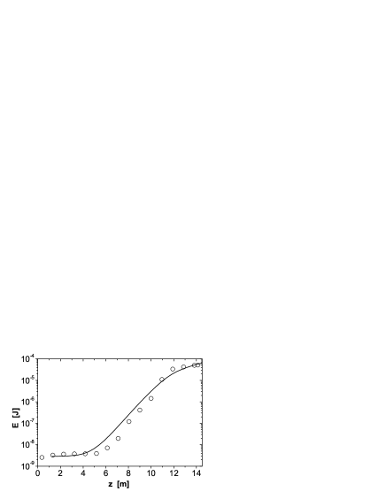
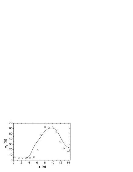
Figure 7: Energy in the radiation pulse (left plot) and fluctuations of the energy in the radiation pulse (right plot) versus undulator length. Circles represent experimental data [2]. Solid lines represent simulation results with code FAST using bunch parameters shown in Fig. 6

Figure 8: Probability distributions of the energy in the radiation pulse for linear (left plot) and nonlinear regime (right plot) regime. Bars represent experimental data [21]. Solid lines represent simulations with code FAST. Dashed line in the left plot shows gamma distribution with the parameter M = 2.6

Left plot in Fig. 8 presents the average energy in the radiation pulse versus undulator length. Details of experiment are presented in [2]. The interaction length has been changed by means of switching on electromagnetic correctors installed inside the undulator. The value of the orbit kick provided by a corrector was sufficient to stop FEL amplification process downstream the corrector. The radiation energy has been measured by means of an MCP-based detector of 10 mm diameter installed 12 m downstream the undulator [22]. When the FEL interaction is suppressed along the whole undulator length, the detector shows the level of spontaneous emission of about 2.5 nJ collected from the full undulator length. In order to reproduce correctly experimental situation, the simulation results were distorted with the same level of noise (5%) as that provided by the radiation detector. Comparison of experimental and simulation results shows reasonable agreement which is within limits of accuracy of experiment. Experimentally measured power gain length is about 70 cm. Calculations of power gain length for the same electron beam without energy chirp give the value which is almost twice shorter, about 40 cm. Explanation of this puzzle is in strong suppression of the FEL gain by the energy chirp in the electron bunch, about 1% on a scale of cooperation length (to be compared with the FEL parameter $\rho$ [19, 20] which is about 0.5%).

Each circle in the left plot in Fig. 8 is the result of averaging over 100 shots. The energy in the radiation pulse fluctuates from shot to shot. The plot for the standard deviation $\sigma$, is presented on the right side in this Figure. At the initial stage fluctuations are defined mainly by the fluctuations of the charge in the electron bunch and the accuracy of measurements. When the FEL amplification process takes place, fluctuations of the radiation energy are mainly given by the fundamental statistical fluctuations of the SASE FEL radiation [23]. A sharp drop of the fluctuations in the last part of the undulator is a clear physical confirmation of the saturation process. Detailed measurement of probability distributions were made for the end of the linear regime (undulator length 9 m), and in the nonlinear regime. A comparison of experimental and simulated probability distributions is presented in Fig. 8. It is seen, as expected from theory[23], that in the linear regime both distributions are gamma-distributions

$$p(E)=\frac{M^{M}}{\Gamma(M)}\left(\frac{E}{\langle E\rangle}\right)^{M-1}\frac{1}{\langle E\rangle}\exp\left(-M\frac{E}{\langle E\rangle}\right)\ ,$$

with the value $M=1/\sigma^{2}\simeq 2.6$ (corresponding to $\sigma=62$% at the undulator length 9 m, see Fig:8). Right plot in Fig. 8 shows comparison of the measured and simulated statistical distributions for the nonlinear regime which again are in excellent agreement.

4.2 Angular divergence

Figure 9 shows the angular divergence of the FEL radiation. Measurements were performed by means of scanning a 0.5 mm aperture across the radiation beam and recording the transmitted intensity on a downstream detector [2]. The simulated curve has been produced by recalculating the radiation field from the near (undulator exit) into the far zone. The agreement between simulation and measurement is perfect: even fine details in the distribution are well reproduced. We can thus state that our simulation model provides the same field distribution at the undulator exit as it was in the experiment. We should emphase that the disagreement in angular distribution presented in a previous analysis [2] was a strong indication on rather complicated physical process. Experimental procedure was very reliable, since it was simple relative measurement of the intensity with respect to maximum. Indeed, we can conclude that long spanning tails in the angular distributions is consequence of the strong longitudinal energy chirp which significantly disturbs the beam radiation mode. Experimentally it was not possible to measure spot size of the radiation at the undulator exit. Right plot in Figure 9 shows relevant distribution reconstructed from the simulation data. Figure 9 led us to the conclusion that there should be a high degree of transverse coherence in the FEL radiation, as it was proven in a dedicated experiment at TTF FEL [24].

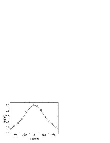
Figure 9: Angular distribution of the radiation intensity in the far zone (left plot) and in the near zone (right plot). TTF FEL operates in the nonlinear regime. Circles represent experimental data [2], and solid curves show results of simulations with code FAST

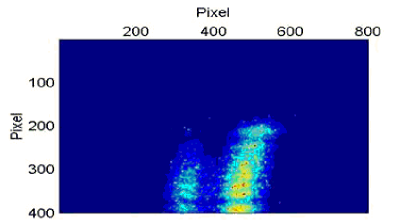
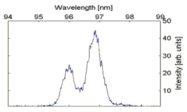
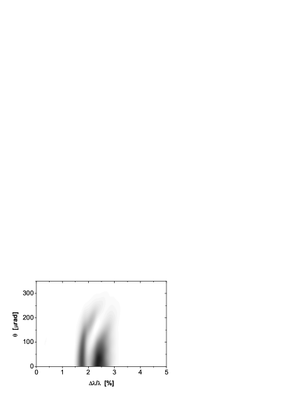
Figure 10: Single shot spectrum for TTF FEL operating in the nonlinear regime. Left column shows image on CCD camera, and right column shows projections. Upper row are experimental data [21] and lower row represents results of simulations with code FAST

4.3 Radiation spectra and fluctuations

The next topic of our study is the radiation spectra. Experimentally such spectra can be measured in a single shot by the mean of a monochromator [25]. In such a measurement the procedure is as follows: the photon beam is deflected by plane mirror, passed through a narrow slit, and then dispersed by a grating. The dispersed beam is then detected by CCD camera as illustrated in Fig. 10 in the left-corner plot. Projection of the CCD readings onto $x$-axis gives the spectrum (see right-corner plot in Fig. 10). The same procedure was reproduced in the simulations and gave the results presented in the lower plots of Fig. 10 . The range of spectral measurements was rather limited due to limited sensitivity of the spectrometer. It was possible to detect reliably single shot spectra in the nonlinear regime, while in the linear regime only spectra, averaged over many shots are available after procedure of background subtraction. In Figure 12 we present comparison of experimental and simulated spectra for nonlinear regime. We again see not only qualitative, but very good quantitative agreement. Note that the bump on the left slope of the average spectra was a signature for all spectral measurements at TTF FEL starting from the first lasing on February 22, 2000 (see Fig. 12). Such a bump is indeed the consequence of the strong energy chirp along the bunch.

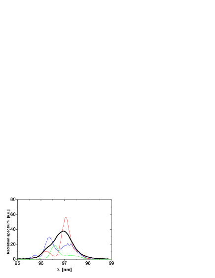
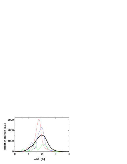
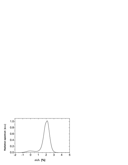
Figure 11: Single shot spectra (thin lines) and averaged spectrum (bold lines) of TTF FEL operating in the nonlinear regime. Left plot shows experimental data [2] and right plot shows results of simulations with code FAST

Figure 12: Average spectrum of TTF FEL operating in the high-gain linear regime. Left plot shows experimental data [26] and right plot shows results of simulations with code FAST

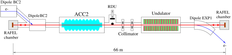
Figure 13: General layout of the experimental facility for measurement of statistical properties of the radiation after narrow-band monochromator. Here BC2 is the bunch compressor, ACC2 is the second accelerating module, RDU denotes the MCP-based radiation detector unit. RAFEL chamber downstream the undulator houses a plane SiC mirror, and the chamber in the BC2 area hoses a grating.

Figure 14: Probability distribution of the energy in the radiation pulse after narrow band monochromator. TTF FEL operates in the linear regime. Left plot shows experimental data with RAFEL grating [21] and right plot shows results of simulations with code FAST. Solid lines show negative exponential distribution

Figure 15: Probability distribution of the energy in the radiation pulse after narrow band monochromator. TTF FEL operates in the nonlinear regime. Left plot shows experimental data with RAFEL grating [21] and right plot shows results of simulations with code FAST

Another important topic of the FEL physics, well documented in the experiment, are the statistical properties of the radiation after narrow-band monochromator. Measurements of fluctuations of the radiation energy after the monochromator have been performed using a narrow-band monochromator of the RAFEL (Regenerative Amplifier FEL [27]) optical feedback system. The scheme for these measurements is shown in Fig. 15 [28]. The SASE FEL radiation emitted by the electron beam is back-reflected by a plane SiC mirror (RAFEL chamber at the right side of the scheme) onto monochromator (RAFEL chamber at the left side of the scheme). The RAFEL monochromator is a spherical grating in Littrow mounting which disperses the light in the direction of the radiation detector unit (RDU) installed 27 meters downstream. The RDU is equipped with an MCP-based radiation detector with a thin (200 $\mu$m) gold wire which plays the role of an exit slit of the monochromator. The design of a spherical grating in Littrow mounting guarantees a resolution of about $(\Delta\omega/\omega)_{\mathrm{M}}\simeq 10^{-4}$ which is much less than typical scale of the spike in spectrum (see Fig. 12). Wide dynamic range of MCP-based radiation detector gave the possibility to perform reliable measurements for both the linear and nonlinear regimes.

In the simulation procedure we also took into consideration aperture limitations along the path of the photon beam (9 mm in the undulator, and 6 mm in the spoiler of the electron beam collimator). The reason for this is that diffraction effects at aperture edges lead to mixing of spectrum which initially was strongly correlated with the angle (see Fig. 10).

The plots in Fig. 15 show the probability distributions of the radiation energy after a narrow-band monochromator. SASE FEL operates in the linear regime, the active undulator length during this measurement was 9 m. When SASE FEL operates in linear regime, the probability density must be a negative exponential distribution:

$$p(E)=\frac{1}{\langle E\rangle}\exp\left(-\frac{E}{\langle E\rangle}\right)\ .$$

The solid curves in Fig. 15 represent the negative exponential distribution. So, we can conclude that both, measured and simulated properties well follow the general properties typical for completely chaotic polarized light.

Theory of SASE FEL predicts that in the saturation regime the fluctuations should drop visibly when pulse duration $T$ is such that $\rho\omega T\lesssim 2$ [29]. At larger values of $\rho\omega T$ fluctuations increase and quickly approach 100% level. Since radiation pulse length of TTF FEL is about two cooperation length, we should expect significant suppression of fluctuations in the nonlinear regime, down to 40%. It is seen in Fig. 15 that measured fluctuations drop drastically in the nonlinear mode of operation of TTF FEL. There is not only qualitative agreement, but also quantitative agreement with calculated probability density distribution function. It is worth to mention that such a stabilization of fluctuations is an independent indication for very short pulse duration $T$ [29].

5 Discussion

The good agreement between experimental data and simulation results allows us to determine the parameters of the FEL which are not directly accessible experimentally. First of all this refers to the temporal structure of the radiation pulse (see Fig. 16): the computed FWHM pulse duration in saturation regime is about 40 fs, and peak power (averaged over ensemble) is 1.5 GW. We can also conclude that the phase 1 of the SASE FEL at the TTF FEL, was driven by strongly non-Gaussian beam having peak current about 3 kA. Beam dynamics in the accelerator (even at high energy, after bunch compressor) was strongly influenced by the space charge effects.

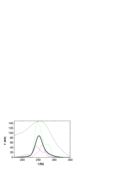
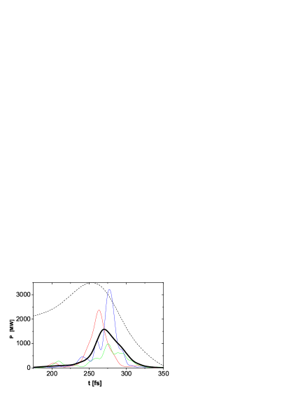
Figure 16: Radiation power along the bunch for TTF FEL operating in the linear (left plot) and nonlinear (right plot) regime. Thin curves show single shots. Bold curves show averaged profiles. Dashed curve shows profile of electron bunch. Simulations are performed with code FAST using bunch parameters shown in Fig. 6

Our simulations show that rather poor transverse emittance of the electron beam originated from the injector. With a large value of emittance, the beam dynamics is not strongly influenced by CSR effects in the bunch compressor. However CSR effects might be a crucial issue for low-emittance beams as foreseen in future X-ray FELs. Strong longitudinal space charge effect was not expected at TTF since local energy spread before compression (parameter defining spike width and peak current after compression) was strongly overestimated. In future machines this effect can be avoided by an appropriate choice of compression schemes. Therefore, the results of our simulations cannot be directly scaled to more advanced accelerator designs for X-ray FELs.

In this paper we did a ”font-end” comparison: we only compared the results of the simulations with the radiation properties which have been measured reliably and with high accuracy. Although direct comparisons of the beam dynamics simulations with the measurements of the slice parameters of the beam at different location along the accelerator would have been more appropriate, there was impossible due to the lack of adequate beam diagnostics. Our rich experimental experience at TTF shows that tuning of the accelerator for the FEL operation is very difficult task without information about relevant beam parameters. Excellent properties of the FEL radiation were mainly achieved by a global empirical optimization of the machine. Such a procedure might be impossible in much larger and more complicated accelerator systems for X-ray FELs with very large parameter space to be tuned. This underlines the urgent necessity to develop electron beam diagnostics tools which are crucial for the proper operation of X-ray SASE FEL. In particular, a method of the peak current and bunch profile reconstruction, based on detection of infrared coherent radiation from an undulator, would perfectly fit this purpose [30]. Reliable methods for measuring slice emittance and energy spread on a femtosecond time scale should be developed, too.

Appendix: Parameters of the leading peak in density distribution created in the bunch compressor due to RF nonlinearity

An expression for the beam density distribution after compression, including RF nonlinearity, was derived in [15]. We present here the simplified formulas for the parameters of the leading peak.

Let us consider a long bunch with the constant current $I_{0}$ accelerated off-crest in an RF accelerator with the RF wavelength $\lambda$. An energy chirp along the beam is

$$E=E_{0}\cos(\phi_{0}+\Delta\phi)$$

Here $\phi_{0}$ is the phase of a reference particle, and $\Delta\phi=2\pi s/\lambda$. A position $s$ of a particle is positive if it is moving in front of the reference particle. We assume that $\Delta\phi\ll 1$ and expand the relative energy chirp up to the second order:

$$\tilde{\delta}=\frac{E-E_{0}}{E_{0}}\simeq-\Delta\phi\tan\phi_{0}-\frac{(\Delta\phi)^{2}}{2}$$ (1)

For a Gaussian uncorrelated energy spread a distribution function in the vicinity of the reference particle can be described as follows:

$$f(s,\delta)=\frac{I_{0}}{\sqrt{2\pi}\sigma_{\delta}}\exp\left[-\frac{\left(\delta+2\pi s\tan(\phi_{0})/\lambda+2\pi^{2}s^{2}/\lambda^{2}\right)^{2}}{2\sigma_{\delta}^{2}}\right]\ ,$$ (2)

where $\sigma_{\delta}$ is the relative rms energy spread. The normalization is chosen such that after integration over $\delta$ we get the current.

Behind the bunch compressor a particle position $s_{f}$ (with respect to a nominal particle) is connected with its position before compression $s_{i}$ and energy deviation $\delta$ as

$$s_{f}\simeq s_{i}+R_{56}\delta+T_{566}\delta^{2}+...\ ,$$ (3)

where $R_{56}$ and $T_{566}$ are the first and the second order momentum compaction. In our consideration we choose the signs such that for a bunch compressor chicane $R_{56}>0$ and $T_{566}\simeq-3R_{56}/2$ (for a small bending angle). It is seen from (1) and (3) that the phase space distribution after compression has a parabolic shape. The reference particle is positioned at the fold-over when

$$\tan(\phi_{0})=\frac{\lambda}{2\pi R_{56}}$$

Also, analyzing Eqs. (1) and (3), we come to the conclusion that the contribution of $T_{566}$ term can be neglected under the condition $\phi_{0}\ll 1$. We also assume that $\sigma_{\delta}\ll\phi_{0}^{2}$. The final distribution function is obtained from (2) by a simple substitution $s\to s-R_{56}\delta$ and is simplified with the help of the above mentioned assumptions:

$$f(s,\delta)=\frac{I_{0}}{\sqrt{2\pi}\sigma_{\delta}}\exp\left[-\frac{\left(s/R_{56}+2\pi^{2}R_{56}^{2}\delta^{2}/\lambda^{2}\right)^{2}}{2\sigma_{\delta}^{2}}\right]\ .$$ (4)

To obtain the dependence of current on s after compression one should make the integration:

$$I(s)=\int\limits_{-\infty}^{\infty}\d\delta\ f(s,\delta)$$

After normalization we get:

$$I(\hat{s})=I_{0}Cg_{1}(\hat{s})\ ,$$ (5)

where

$$\hat{s}=\frac{s}{R_{56}\sigma_{\delta}}\ ,\ \ \ \ C=\frac{\lambda}{\pi R_{56}\sqrt{2\sigma_{\delta}}}\ ,$$

and the function $g_{1}(\hat{s})$ is

$$g_{1}(\hat{s})=\sqrt{\frac{2}{\pi}}\int\limits_{0}^{\infty}\d x\exp\left[-\frac{(\hat{s}+x^{2})^{2}}{2}\right]\ .$$ (6)

The plot of the function $g_{1}(\hat{s})$ is presented in Fig. 17. The maximal value of the function $g_{1}(\hat{s})$ is close to 1, $\mathrm{max}(g_{1}(\hat{s}))\simeq 1.02$, so that $C$ describes the enhancement of current. The full width (at half maximum) of this curve is 4.8, or in dimensional notations:

$$(\Delta s)|_{\small\mathrm{FWHM}}\simeq 4.8R_{56}\sigma_{\delta}$$ (7)

At the level of 0.8 the full width $\Delta\hat{s}$ is equal to 2. We can also estimate the length of the beam slice before compression, contributing to the leading peak after compression - it is of the order of $\lambda\sqrt{\sigma_{\delta}}$. Thus, if the current (before compression) only weakly changes on this scale, our approximation of constant current is valid.

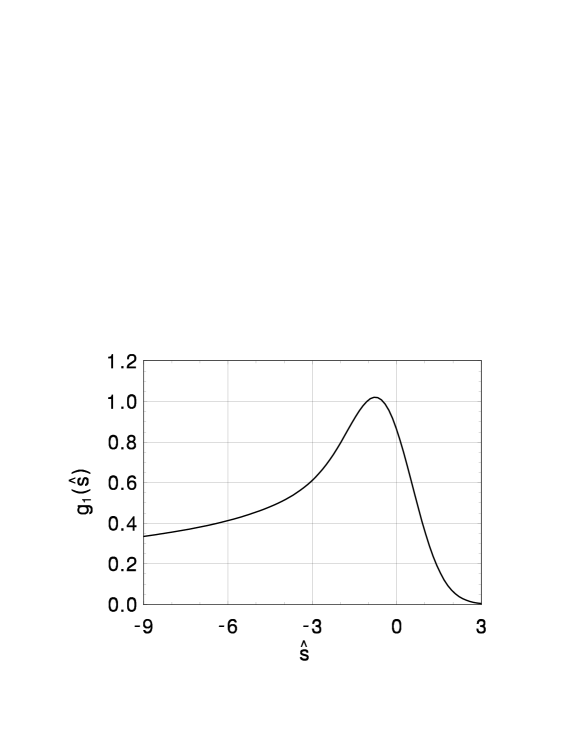
Figure 17: Function $g_{1}(\hat{s})$

It is interesting to know the slice energy spread after compression. It is easy to obtain from (4) the following result:

$$\delta_{\mathrm{rms}}(\hat{s})=\sigma_{\delta}Cg_{2}(\hat{s})\ ,$$ (8)

where

$$g_{2}(\hat{s})=\left[\frac{\int\limits_{0}^{\infty}\d xx^{2}\exp\left[-(\hat{s}+x^{2})^{2}/2\right]}{\int\limits_{0}^{\infty}\d x\exp\left[-(\hat{s}+x^{2})^{2}/2\right]}\right]^{1/2}$$ (9)

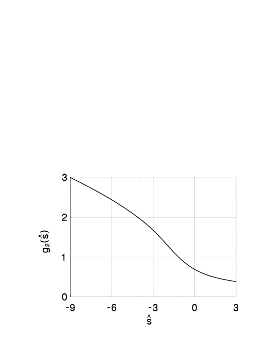
Figure 18: Function $g_{2}(\hat{s})$

The plot of this function is presented in Fig. 18 In the slice with maximum current, $\hat{s}=-0.8$, the function $g_{2}$ takes the value of 0.89. The ratio

$$\frac{I(s)}{\delta_{\mathrm{rms}}(s)}=\frac{I_{0}}{\sigma_{\delta}}\frac{g_{1}(\hat{s})}{g_{2}(\hat{s})}$$

can be important for FEL operation. In Fig. 19 we plot the function $g_{1}(\hat{s})/g_{2}(\hat{s})$. One can see some enhancement of the ratio of local current to slice energy spread with respect to uncompressed beam. The full width of the curve is about 3, beyond this good range it quickly goes down, so that only a small part of the beam is favorable for lasing (if it is not spoiled by collective effects). Note that rms energy spread is an adequate quantity for SASE FEL calculation when it is much less than the FEL parameter $\rho$ [19, 20]. When it becomes comparable to $\rho$, one should take into account the actual distribution (to know only dispersion is not sufficient). When it is much larger that $\rho$, one can think of two independent beams, having different energies and twice lower current.

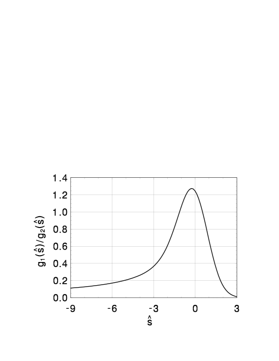
Figure 19: The ratio $g_{1}(\hat{s})/g_{2}(\hat{s})$

Finally, let us present a numerical example. An electron beam with the current 80 A and rms energy spread 3.5 keV is accelerated up to 135 MeV in the RF accelerator with $\lambda=23$ cm. After that it is compressed in a bunch compressor with $R_{56}=23$ cm. The peak current after compression is then 3.6 kA, rms energy spread in the slice with maximum peak current is about 140 keV, and full width of the leading peak is 28 $\mu$m.

References

- [1] V. Ayvazyan et al., Preprint DESY 01-226, DESY, Hamburg, 2001.
- [2] V. Ayvazyan et al., Phys. Rev. Lett. 88(2002)104802.
- [3] V. Ayvazyan et al., Eur. Phys. J. D20(2002)149
- [4] W. Brefeld et al., Nucl. Instrum. and Methods A393(1997)119.
- [5] S. Schreiber et al, Proceedings EPAC2002, Paris, France, p.1804.
- [6] M. Huening and H. Schlarb, “Measurements of the beam energy spread in the TTF photoinjector”, in Proc. of PAC2003.
- [7] S. Schreiber et al, Proceedings EPAC2000, Vienna, Austria, p.309.
- [8] M. Huening, Proc. 5th European Workshop on Diagnostics and Beam Instrumentation, May 2001, Grenoble, France, p.56.
- [9] K. Flöttmann, Astra User Manual, http://www.desy.de/ mpyflo/Astra_dokumentation/
- [10] M. Borland, ”elegant: A flexible SDDS-Compilant Code for Accelerator Simulation”, APS LS-287, September 2000
- [11] M. Dohlus, private communication.
- [12] E.L. Saldin, E.A. Schneidmiller and M.V. Yurkov, Nucl. Instrum. and Methods A429(1999)233.
- [13] E.L. Saldin, E.A. Schneidmiller and M.V. Yurkov, Nucl. Instrum. and Methods A398(1997)373.
- [14] P. Emma and G. Stupakov, in Proc. of EPAC2002, Paris, 2002, p.1479.
- [15] R. Li, Nucl. Instrum. and Methods A475(2001)498.
- [16] E.L. Saldin, E.A. Schneidmiller and M.V. Yurkov, Nucl. Instrum. and Methods A490(2002)1.
- [17] S. Heifets, G. Stupakov and S. Krinsky, Phys. Rev. ST Accel. Beams 5(2002)064401
- [18] Z. Huang and K.-J. Kim, Phys. Rev. ST Accel. Beams 5(2002)074401
- [19] R. Bonifacio, C. Pellegrini and L.M. Narducci, Opt. Commun. 50(1984)373.
- [20] E.L. Saldin, E.A. Schneidmiller and M.V. Yurkov, The Physics of Free Electron Lasers, Springer-Verlag, Berlin, 1999.
- [21] V. Ayvazyan et al., Nucl. Instrum. and Methods A507(2003)368.
- [22] B. Faatz et al., DESY Print TESLA-FEL 2001-09, pp. 62-67.
- [23] E.L. Saldin, E.A. Schneidmiller and M.V. Yurkov, Opt. Commun. 148(1998)383.
- [24] R. Ischebeck et al., Nucl. Instrum. and Methods A507(2003)175.
- [25] R. Treusch et al., Nucl. Instrum. and Methods A467-468(2001)30.
- [26] J. Andruszkow et al., Phys. Rev. Lett. 85(2000)3825.
- [27] B. Faatz et al., Nucl. Instrum. and Methods A429(1999)424.
- [28] M.V. Yurkov et al., Nucl. Instrum. and Methods A483(2002)51.
- [29] E.L. Saldin, E.A. Schneidmiller and M.V. Yurkov, Nucl. Instrum. and Methods A507(2003)101.
- [30] G. Geloni et al., Preprint DESY 03-031, DESY, Hamburg, 2003.