Progress in Classical and Quantum Variational Principles.111Reports on Progress in Physics (2004)
Abstract
We review the development and practical uses of a generalized Maupertuis least action principle in classical mechanics, in which the action is varied under the constraint of fixed mean energy for the trial trajectory. The original Maupertuis (Euler-Lagrange) principle constrains the energy at every point along the trajectory. The generalized Maupertuis principle is equivalent to Hamilton’s principle. Reciprocal principles are also derived for both the generalized Maupertuis and the Hamilton principles. The Reciprocal Maupertuis Principle is the classical limit of Schrödinger’s variational principle of wave mechanics, and is also very useful to solve practical problems in both classical and semiclassical mechanics, in complete analogy with the quantum Rayleigh-Ritz method. Classical, semiclassical and quantum variational calculations are carried out for a number of systems, and the results are compared. Pedagogical as well as research problems are used as examples, which include nonconservative as well as relativistic systems.
“…the most beautiful and important
discovery of Mechanics.”
Lagrange to Maupertuis (November 1756)
1 Introduction and History
Variational Principles have a long and distinguished history in Physics. Apart from global formulations of physical principles, equivalent to local differential equations, they also are useful to approximate problems too difficult for analytic solutions. In the past century quantum variational calculations have been ubiquitous as an approximate method for the ground state of many difficult systems . In recent years there has been some progress in using classical variational principles (Action Principles) to approximate the motion of classical systems such as classical molecules. We review recent developments in this area of Classical Mechanics, although we also overlap with Quantum Mechanics. In particular we shall also discuss the use of the quantum variational principle for excited states, and the connection to classical action principles.
In Classical Mechanics, variational principles are often called Least Action Principles, because the quantity subject to variations is traditionally the Action. To confuse matters there are two classical Actions, corresponding to two main Action Principles, which are called respectively, Hamilton’s Action and Maupertuis’ Action ; these differ from each other (they are related by a Legendre transformation), and the notation is not universal (we follow current usage but in fact some authors use the same symbols reversed [2]). Both Actions, and , have the same dimensions (i.e. energytime, or angular momentum). Maupertuis’ Least Action Principle is the older of the two (1744) by about a century, and as we shall discuss, it is inconveniently formulated in all textbooks [3]. For clear statements of these old action principles, see the textbooks by Arnold [4], Goldstein et al [5], and Sommerfeld [6]. We shall review these Action Principles in the next section. Some mathematics and notation required to deal with variational problems are summarized in Appendix I. The distinguishing feature of variational problems is their global character [7]. One is searching for the function which gives a minimum (or stationary value) to an integral, as opposed to local extrema, where one is searching for the value of the variable which minimizes ( or makes stationary) a function. Of course this dichotomy is not so sharp in practice, as the global problem is equivalent to a differential equation (the Euler-Lagrange equation) which is of course local. The relation has even found its way into modern parlance [8]: “Think globally, act locally!”.
In Quantum Mechanics, where (usually) the aim is for approximations to the energy by choosing a wave-function, one speaks of trial wave-functions, which are optimized according to a Variational Principle. In Classical Action Principles, the equivalent notion is that of a virtual path or trajectory, which should be optimized in accordance with the Action Principle. For uniformity we shall talk of Trial Trajectories in the classical domain, to emphasize the similarity of these ideas.
As noted above, Maupertuis’ Action Principle was formulated in precise form first by Euler and Lagrange some two and a half centuries ago; for the history, see the books by Yourgrau and Mandelstam and by Terral [9]. However, even the formulation of these eminent mathematicians remained problematic, as emphasized by Jacobi, who stated in his Lectures on Dynamics: “ In almost all text-books, even the best, this Principle is presented so that it is impossible to understand” [10, 11]. To understand at least in part the problem (see [12] for a detailed discussion), it is sufficient to note that Maupertuis’ Principle assumes conservation of energy, whereas a well formulated principle, like Hamilton’s Principle, implies energy conservation. As we shall see, it is possible to reformulate Maupertuis’ Principle in a more general form to remedy this problem and also make it more useful in applications [12, 13]. It should be noted that Hamilton’s Principle does not suffer from any such drawbacks and is useful both conceptually (to derive equations of motion) and as a tool for approximations. The reformulated Maupertuis Principle has the advantage of being closely related to the classical limit of Schrödinger’s Variational Principle of wave mechanics, and thereby lends itself easily to semiclassical applications.
Even though we emphasize two Action Principles for Classical Mechanics, it is worth noting that there are many other formulations and reformulations of these principles. For a list of references on this point see ref.[12]. We note in particular the elegant work of Percival in the 1970’s on variational principles for invariant tori (see ref.[14] for a review). The emphasis on Maupertuis and Hamilton reflects the two main approaches of mechanics, one based on the Lagrangian and the other based on the Hamiltonian .
In the above and in section 2 we use the traditional terminology for the variational principles, i.e. “least” action principles, but, since Jacobi’s work it has been recognized [4, 11] that the action is in fact stationary in general for the true trajectories. This means the first-order variation vanishes, and the action may be a minimum, a maximum or a saddle, depending on the second-order variation [15]. Hence “stationary” action principles would be more accurate terminology. Similar remarks apply to the general Maupertuis and reciprocal variational principles discussed in section 2.
In sections 2-4 we restrict ourselves to conservative holonomic systems. Various problems are solved using classical and semiclassical variational methods and some comparisons are made with the results from the quantum variational method for excited states [16]. In section 5 we discuss nonconservative (but nondissipative) systems, and in section 6 we mention briefly particular nonholonomic systems (which have velocity constraints), in connection with relativistic systems. The relations between classical and quantum variational principles (VP’s) are discussed in section 7.
2 Action Principles of Classical Mechanics
2.1 Statements of Action Principles
Hamilton’s Least Action Principle (HP) states that, for a true trajectory of a system, Hamilton’s Action is stationary for trajectories which run from the fixed initial space-time point to the fixed final space-time point ,
where is the duration. Here the (Hamilton) action is the time integral of the Lagrangian from the initial point to the final point on the trial trajectory ,
where is the generalized coordinate, the generalized velocity and the time. In practice we choose and for convenience. In general stands for the complete set of independent generalized coordinates , where is the number of degrees of freedom [17]. In (2.1) the constraint of fixed is indicated explicitly, but the constraint of fixed end-positions and is left implicit. The latter convention for the end-positions is also followed below in (2.2), (2.3), etc. From the Action Principle (2.1) one can derive Lagrange’s equation(s) for the trajectory, which we shall not do in this review; see for example [4, 5, 6].
The reformulated (or General) Maupertuis Least Action Principle (GMP) states that, for a true trajectory Maupertuis’ Action is stationary on trajectories with fixed end-positions and and fixed mean energy :
Here Maupertuis’ Action is given by
where is the canonical momentum, and in general stands for . The second form for is valid for normal systems, for which and is quadratic in the ’s, where is the kinetic energy and the potential energy. The mean energy is the time average of the Hamiltonian over the trial trajectory of duration ,
from the initial position to the final position which are common to all trial trajectories. Note that is fixed in (2.2) but is not, the reverse of the situation in (2.1). We use the notation rather than because in the early sections we restrict [18] ourselves to dynamical variables where the Hamiltonian is equal to the energy ; the general case is discussed in note [19] and later sections.
The Reciprocal Maupertuis Principle (RMP), or principle of least (stationary) mean energy, is
For stationary (i.e. steady-state or bound) motions (periodic, quasiperiodic, chaotic) (2.3) is the classical limit [12] of the Schrödinger Variational Principle of Quantum Mechanics: , (see also sec.7). The connection is clear intuitively: for bound motions, in the large quantum number limit the expectation value of the Hamiltonian becomes the classical mean energy and the quantum number becomes proportional to the classical action over the motion. This connection enables the RMP to lend itself naturally to semiclassical applications (sec. 2.3). For periodic and quasiperiodic motions the Reciprocal Maupertuis Principle (2.3) is equivalent [12] to Percival’s principle for invariant tori [14, 20] . The RMP is, however, more general and is valid for chaotic motions, scattering orbits, arbitrary segments of trajectories, etc. Percival’s principle has been derived by Klein and co-workers from matrix mechanics [21] in the classical limit. Hamilton’s Principle also has a reciprocal version [12] - see next section. For a summary of reciprocity in variational calculus, see Appendix I.
The textbook Euler-Lagrange version of Maupertuis’ Principle differs from (2.2); the constraint of fixed mean energy is replaced by one of fixed energy ,
This is not erroneous, since a true trajectory does indeed conserve energy, but it is the source of the inconveniences referred to by Jacobi [11]. Because, as we show in the next section, the GMP is equivalent to the HP, and therefore to the equations of motion from which energy conservation follows, it will become clear that energy conservation is a consequence of the GMP (2.2), rather than an assumption as in the original MP (2.4).
It is well known that conservation of energy is a consequence of symmetry under time translation (Noether’s theorem), either via the Lagrangian and equations of motion [22] , or from the action and Hamilton’s Principle [23]. Similarly energy conservation can be derived directly from the GMP [12].
In the early sections we assume and that is time-independent (conservative). Later these restrictions are relaxed (see sections 5 and 6).
2.2 Derivation of Action Principles
Within Mechanics one can show that different Action Principles such as (2.1), (2.2) and (2.3) are equivalent to each other. This we sketch below (see [12] for more details). Alternatively, one can show [4, 5, 6] from Hamilton’s Principle (2.1) that the Lagrange equations of motion, in some coordinates are essentially Newton’s equations in the same set of coordinates. Reference [9] shows that (2.4) is equivalent to Newton’s equations, quoting an argument due to Lagrange, and in [12] we derive (2.3) from similar arguments. On a more lofty level one can derive the Action Principles from Quantum Mechanics in the classical limit. Dirac and Feynman [24] have derived Hamilton’s Principle from a path integral formulation of Quantum Mechanics, and similarly the RMP (2.3) can be derived from wave mechanics (see [12]). Further connections between quantum and classical variational principles are given in sec. 7.
The equivalence of Hamilton’s Principle (2.1) with the General Maupertuis Principle (2.2) is worth spelling out in a little more detail. (The equivalence of the MP with the GMP is discussed in Appendix II). The starting point of the derivation is the Legendre transformation between the Lagrangian of the system and the corresponding Hamiltonian,
Here runs over the various degrees of freedom, and stands for and for . Upon integration over time along a trial trajectory starting at and ending at (where we could have for a closed trajectory), and with the definitions given above we obtain
where is the duration along the trial trajectory. Thus and are also related by a Legendre transformation. If we now vary the trial trajectory and the duration , keeping and fixed, and compute the variation of the different terms in (2.6), we obtain
which is the relation between the different variations. For conservative systems, near a true trajectory Hamilton’s Principle is equivalent to the vanishing of the left hand side. In fact a vanishing left hand side is the unconstrained form [25] of Hamilton’s Principle (the UHP - see [12] for proof):
where we have used the fact on a true trajectory for conservative systems. Eq (2.8) has the unconstrained form , with (the energy of the true trajectory) a constant Lagrange multiplier. For fixed (i.e. ), we recover the HP , and for fixed (i.e. ) we obtain the Reciprocal Hamilton Principle (RHP)
The RHP (principle of least time) is discussed in detail in ref.[12].
The right hand side of (2.7) (which therefore must also vanish near a true trajectory) gives the unconstrained form of Maupertuis’ Principle (UMP) for conservative systems:
This has the unconstrained form , with ( the duration of the true trajectory) a constant Lagrange multiplier. For fixed (2.10) gives the GMP of equation (2.2) while for fixed it gives the reciprocal, the RMP of equation (2.3). An alternative derivation of the UMP (2.10) is given in ref.[12] with traditional variational procedures, employing the general first variation theorem of variational calculus, which includes end-point variations [15, 29].
Equation (2.7) connecting the different variations is reminiscent of equations of thermodynamics, where two conditions are derived from a single equation. There are many other analogies with thermodynamics, e.g. two actions in mechanics analogous to two free energies in thermodynamics, with a Legendre transform relation in each case [26], adiabatic processes and reversible processes in both mechanics and thermodynamics, and reciprocal variational principles in both mechanics and thermodynamics (see Appendix I). Beginning with Helmholtz [9], many of these analogies have been explored by various authors [27].
As we have stressed, we hold the end-positions and fixed in all the variational principles discussed above. It is possible to relax these constraints by generalizing further the UHP and UMP (see notes [25], [26], and [124]), but we shall not need these generalizations for the applications we discuss.
The derivation we have sketched shows that the four principles (2.1), (2.2), (2.3), (2.9) are equivalent to each other. Mathematically, the Hamilton Principles can be regarded as Legendre transformations of the Maupertuis Principles, since the Legendre transformation relation allows us to change independent variables from to . Thus in Classical Mechanics we have a set of four variational principles that are symmetric under Legendre and reciprocal transformations:
After a short interlude on action principles in semiclassical mechanics we proceed to discuss some simple examples.
2.3 Semiclassical Mechanics from Action Principles
The RMP ( 2.3) is the basis of a very simple semiclassical quantization method. As we shall see, the solution of (2.3) yields, for the true trajectory or approximations to it, as a function of the action , . For bound motions we then assume the standard Einstein-Brillouin-Keller (EBK) [28] quantization rule for the action over a cycle
where , is essentially the Morse-Maslov index ( e.g. for a harmonic oscillator), and is Planck’s constant. (EBK (or torus) quantization is the generalization of Bohr-Sommerfeld-Wilson quantization from separable to arbitrary integrable systems). Thus we have expressed as a function of the quantum number , . For multidimensional systems, (2.11) is applied to each action in , so that we get as a function of the quantum numbers . This method has been found to be reasonably accurate even for nonintegrable systems, where strictly speaking the good actions do not exist. The UMP (2.10) can also be used to obtain semiclassical expressions for . Examples are given later in sections 4.1 - 4.3.
3 Practical Use of Variational Principles. Pedagogical Examples
Here we discuss how to use variational principles to solve practical problems. We use the so-called direct method [29] of the calculus of variations (e.g. Rayleigh-Ritz), which operates directly with the variational principle and makes no use of the associated Euler-Lagrange differential equation. Historically [30], the method originates with Euler, Hamilton, Rayleigh, Ritz and others (see [12, 29] for some early references).We assume a trial solution, which contains one or more adjustable parameters . We then use the variational principle to optimize the choice of the . Generally speaking, the more parameters , the better the solution. The direct method is well known in quantum mechanics, but is also very useful in classical mechanics, as we shall see. We give a few simple examples in this section, mainly for bound motions; further simple examples, including for scattering problems, are given in refs. [12, 13] and in the references therein .
The simplest example is the free motion of a particle of unit mass on the line segment to . With the traditional Maupertuis principle (2.4) once we fix the energy there is essentially nothing left to vary. With the GMP (2.2) or its reciprocal (2.3) we can choose a variety of trial trajectories. For example we can take velocity on the sub-segment and velocity on the sub-segment . The action is and the mean energy is , where we can vary to change while keeping the mean energy fixed. We then find that , a simple example of energy conservation for this particular trial trajectory. By iteration we can now see that energy is conserved for the whole trajectory on the segment , as a consequence of the General Maupertuis Principle (2.2).
3.1 The Quartic Oscillator
An instructive example is the one-dimensional (1D) quartic oscillator, with Hamiltonian
Using a harmonic oscillator trial trajectory with
we find for a complete cycle with period
From (3.3), with the use of the RMP (2.3) we can obtain the “best” frequency solving , which can be substituted into (3.3) to obtain
and the period as a function of mean energy:
This variational estimate for the period is in error by when compared with the exact result, as noted in reference [13]. Systematic improvements can be obtained by including terms , , etc., in the trial trajectory ; see [13] for a related example.
We have used the RMP here since (3.3) made it very convenient to do so. The GMP and the HP are also viable for this problem, but the original MP is not, since the constraint of fixed leaves essentially no freedom for variation for 1D problems [31]. One can get around this by relaxing the constraint via a Lagrange multiplier, but this is then equivalent to the GMP (see App. II) or the UMP. In 2D etc., the constraint of fixed does allow some freedom for variation, but the constraint is very cumbersome and the GMP is always much more convenient.
The use of the action principle (2.3) to obtain the mean energy as a function of the action (3.4) or the period as a function of mean energy (3.5), with harmonic oscillator trial trajectories, is very similar to the use of the variational principle in quantum mechanics to estimate the energies of states of the quartic oscillator with harmonic oscillator trial wave-functions. We show this explicitly for the eigenstates of the Hamiltonian (3.1). In both cases an optimum frequency for the trial harmonic case is sought and the final errors are also similar. We start by computing the quantum expectation value of (3.1) using a harmonic oscillator state with trial frequency ,
and find the optimum frequency by demanding the vanishing of the derivative of with respect to the frequency. We substitute this frequency in (3.6) to estimate the energy of excited states
Taking the asymptotic limit of (3.7) for and replacing by we obtain the second equation (3.4). This is not as trivial as it seems, since (3.7) was obtained from the quantum variational principle (for an arbitrary state [16]), while (3.4) was obtained from a classical action principle.
This example illustrates neatly that the two variational principles are related: the Reciprocal Maupertuis Principle is the classical limit of the Schrödinger Variational Principle (see sec.7 for further discussion). The example illustrates also that the classical action principle can be used as a method of approximation, and semiclassically to estimate as described in sec.2.3. According to (2.11), we quantize in (3.4) semiclassically by the replacement ; as just discussed, this leads to agreement asymptotically ( ) with the quantum result (3.7). Reference [16] discusses the similar relation between quantum and classical variations for a different one-dimensional system, with a linear potential. The application of classical action principles to other simple systems is discussed in reference [13]. The application of quantum variations for excited states has a long history: the earliest reference is McWeeny and Coulson, who applied it to the quartic oscillator described above [32] more than fifty years ago (for later references see [16]).
3.2 The Spherical Pendulum. Precession of Elliptical Orbits
For a pendulum with two degrees of freedom (), there is an additional term in the kinetic energy compared to that of a plane pendulum, i.e.
where is the polar angle (measured from the downward vertical axis) and is the azimuthal angle, is the bob mass, the length, and the gravitational acceleration.
Using the axial symmetry around the (vertical) axis, we introduce the cylindrical coordinate , and the angular momentum component , which is a constant of the motion. We also expand , keeping up to quartic terms, which are . This gives
where . With two degrees of freedom and two constants of the motion ( and the energy), the system is integrable.
If the quartic terms are neglected in (3.9) by assuming , the or motion is that of a 2D isotropic harmonic oscillator with frequency . In particular, an elliptical orbit, with semiaxes and , is fixed in space, and the motion is periodic. If the quartic terms are not negligible, the oscillator frequency shifts from to a lower value , as in the plane pendulum case, where
and the orbit precesses in the prograde sense with frequency , where
The motion is now in general quasiperiodic. The precession is one of the major sources of error to be eliminated in the design of Foucault pendula [33]. (The Foucault pendulum is discussed in Sec. 5.2.2.) Because the precession rate is , this precession is particularly relevant for recently developed short Foucault pendula, which are less than 1 m in length. Equations (3.10) and (3.11) have been derived by perturbation theory [34].
To derive (3.10) and (3.11) variationally [13], we first choose a trial trajectory; we take an ellipse which is closed in the coordinate system which rotates with respect to the fixed system with the (unknown) precession frequency . In the system we therefore have and , where may differ from . Because the and systems differ by a rotation, we have , and therefore our trial trajectory in the fixed coordinate system is
To apply the Maupertuis principles, we calculate the action and mean energy over one period of the rotating ellipse,
where denotes a time average over one period, and and are given by (3.9). The averages of the terms in (3.9) are easily calculated using (3.12), which gives
The precession frequency can be related to the angular momentum using , and from (3.14), giving
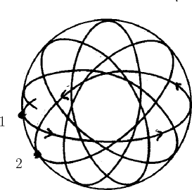
As initial and final positions 1 and 2 (see Fig.1), we take two successive aphelia at , i.e. and , where .The positions 1 and 2 and hence and are thus fixed, which leaves and available as variational parameters. Note that (3.15) then implies that is varied with the trial trajectory (although it is a constant of the motion on the individual trial trajectories). We find it easiest to use the unconstrained version of the Maupertuis principles [i.e. the UMP (2.10)], , where is the time to reach position 2 from position 1. Thus we use
where, choosing units such that , , , we have from (3.13) to (3.15)
and
The first of the variational equations (3.16) is satisfied identically by (3.17) and (3.18), and gives no useful information. From the second, setting , where is the frequency shift, and retaining terms only to second order in and , i.e., in general units, we get the condition
When , (3.19) gives as it should [recall the plane pendulum result [12, 13]]. By symmetry, must reduce to when . This requires that in (3.19), and from this result we then get from (3.19). When we restore the dimensional quantities and , these results agree with (3.10) and (3.11), so that with a harmonic oscillator trial trajectory, the variational method gives results correct to .
Hamilton’s Principle can also be applied to this problem. Here, we need the Hamilton action , where (and hence ) is now fixed, in addition to the positions 1 and 2 (and hence and ). This leaves available as a variational parameter, and setting leads to the same results as above.
4 More Complicated Examples. Research Problems
More complicated examples are easy to find, and are especially interesting in multidimensional systems which exhibit chaotic motion. Such systems are nonintegrable, and have fewer constants of the motion than the number of degrees of freedom. We illustrate the use of classical and semiclassical variational principles together with the application of quantum variational principles to excited states.
4.1 The oscillator
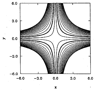
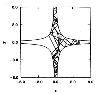
The 2D oscillator is a simple example of this class, which has been studied in the literature for some time (see, e.g. [35, 36]). There is only one constant of the motion, the energy. Classically, most trajectories in this system are chaotic [37]. Fig.2 shows the contours of the potential, and Fig.3 shows a typical (chaotic) classical trajectory.
Refs.[12, 13] give classical and semiclassical discussions of the motion using the RMP. Here we discuss the quantum states using variational methods for the excited states, as done above for a simpler example. Comparison with the semiclassical results is given later. The Hamiltonian is
We choose units where and , where is the potential. Below we also choose . We take as an approximation a separable trial wave-function
where the wave-function is an eigenstate of a harmonic oscillator with frequency :
The frequencies and are variational parameters, which will differ from state to state, and as a result the set (4.2) is nonorthogonal. The computation of matrix elements and expectation values with the wave functions (4.3) is rather easy,
and therefore the expectation value of the Hamiltonian (4.1) with the wave-functions (4.2) is
We then find the best frequencies and by setting to zero the partial derivatives of with respect to the two ’s to obtain the frequency conditions
from which we obtain
Eqs. (4.7) and (4.3) show that at the variational minimum the ratio of the two frequencies is rational and the mean energy of the -oscillator is the same as the mean energy of the -oscillator. It follows immediately that the mean kinetic energies of the two oscillators are also equal to each other at the variational minimum: . From (4.6) we also find
which gives the separate frequencies
and the variational estimate for the energy:
Therefore the variational states are labelled by the two integers and and the energy at high quantum numbers increases as the two thirds power of their product.
The estimate (4.10) can also be obtained semiclassically by using the RMP to find , and then quantizing the actions with the EBK relation (2.11); see ref.[13] for a detailed discussion. It is to be noted that this method yields the quite reasonable first approximation (4.10) for despite the fact that strictly speaking the good actions and do not exist for the oscillator. In essence, one is approximating a chaotic trajectory by a quasiperiodic one, and the RMP picks out the best such trial trajectory [38].
The estimate (4.10) differs only in the leading coefficient , 3/2 vs. 1.405, from a semiclassical adiabatic formula (SCA) obtained by Martens et al [35]. The difference between the two estimates is about . As noted by Martens et al [35] formula (4.10) gives rise to degeneracies. For example = (7,0), (0,7), (2,1), (1,2) give the same energies - a four-fold degeneracy. However, numerical estimates of the first 50 energy levels, obtained in [35], do not show such high degeneracies. Also, because the symmetry group of the Hamiltonian (a fourfold axis of rotation, and four reflection planes) has only one- and two-dimensional irreducible representations [39], we expect at most two-fold degeneracy. We shall see that the basis (4.2) permits an evaluation of the splitting of these spurious degeneracies. The pattern of degeneracies is easy to understand if the bracket is rewritten
where the number (the“principal” quantum number), is an odd integer. The degeneracy pattern is determined by the decomposition of into prime factors. For example =(2,1) corresponds to =15 which can be factored as , , , and these products correspond to (7,0) etc. If is a prime number there are only two states, corresponding to and , while every nontrivial factorization of a nonprime allows further states. The integer belongs to one of two possible classes: or . For the case (e.g. =15) one of is even and the other is odd. This class of states EO and OE (of [35]) corresponds to the two dimensional irreducible representation of . For ( e.g. =21) the two quantum numbers are both even or both odd (e.g. = (10,0) or (0,10) or (1,3) or (3,1) for =21, which is therefore four-fold degenerate). This degeneracy is split into states of symmetry EEE, EEO, OOE and OOO, in the notation of Martens et al [35] for the one dimensional irreducible representations. In this notation the first two letters give respectively the parity ( Even or Odd) of and (or equivalently the behaviour of the wave-function under the reflections (, ), while the third letter stands for the behavior under the interchange of with . We discuss later the splitting of degeneracies resulting from the expression (4.10). At this point we wish only to note that the degeneracy grows very slowly with , like lnln, and even for quite large where quasiclassical behaviour is expected (say ) the typical number of degenerate states is quite modest, 4 - 6.
The main points of discussion arising from the result (4.10) are the splitting of the degenerate levels, perturbative corrections to the variational energies , and the density of states implied by this formula. For the first fifty low lying states one has the accurate numerical estimates of Martens et al [35] with which to compare.
4.1.1 Perturbative Shift of Variational Results
We can improve the variational result (4.10) if we rewrite the Hamiltonian (4.1) in the form
Here, the perturbation is the last term above, and its effect is already included in first order, in the variational estimate (4.10). Therefore the first correction comes in second order in . We must also remember that that the frequencies are appropriate to a fixed pair of quantum numbers , and change if we go to a different pair. The simplest way to do perturbation theory in these circumstances is to estimate corrections to each state by considering a set of orthogonal intermediate states all with the same frequency appropriate to the state which we consider. Therefore we take the second order correction
Due to the form of (quadratic in the coordinates ), we must have or or for nonzero contributions and similarly for . It is an interesting property of the variational solution that only intermediate states with both different from and different from give nonvanishing contributions, because of the frequency conditions. This can be seen from an evaluation of matrix elements with only one quantum number different, for example , but . Then one finds
and the bracket on the right hand side vanishes because of (4.6). Only the perturbation contributes to nonvanishing matrix elements. There are only four intermediate states which contribute: , where , etc. Therefore (4.12) becomes after a little computation
and
where denotes a second-order shift and denotes the energy up to the second-order.
Therefore, in second-order perturbation theory, the coefficient is diminished by about to 1.437, closer to the adiabatic result 1.405 of Martens et al [35] . The remaining difference is about . The degeneracies of (4.14) are still the same as those of (4.10). If we apply perturbation theory to the ground state we find
The sequence (4.15) indicates that the perturbation expansion does not converge, and it is a good idea to stop at second order. The accurate numerical result for (from [35]) is 0.5541, which shows that stopping at second order gives an error of about for the ground state.
Some examples of the estimates , and are given in Table 1, and compared with numerical estimates from [35], for a set of states which are also relevant to the next section.
Table 1
| 1 | (0,0) | 0.5541 | 0.595 | 0.570 | 0.5577 | |
|---|---|---|---|---|---|---|
| 5 | (2,0) | 1.7575 | 1.7406 | 1.6681 | 1.7471 | 1.6308 |
| 9 | (4,0) | 2.4920 | 2.5756 | 2.4683 | 2.5377 | 2.4132 |
| 13 | (6,0) | 3.1180 | 3.2911 | 3.1540 | 3.2171 | 3.0836 |
| 17 | (8,0) | 3.6909 | 3.9357 | 3.7717 | 3.8309 | 3.6874 |
| 21 | (10,0) | 4.2504 | 4.5310 | 4.3422 | 4.3973 | 4.2453 |
| 25 | (12,0) | 5.0490 | 5.0895 | 4.8775 | 4.9297 | 4.7685 |
| 29 | (14,0) | 5.3327 | 5.6189 | 5.3847 | 5.4347 | 5.2645 |
EEE states at low excitation. The exact values and are taken from [35]; the variational estimates and second order results correspond to formulae (4.10) and (4.14), while the are obtained following section 4.1.2
4.1.2 Splitting of Degenerate States
The basis (4.2) is also quite convenient to obtain the splitting of degenerate states. We shall deal with the simplest example with a degeneracy: the pair of states and . Both these states have the same energy in the variational approximation. The wave-functions of the two states are nonorthogonal, because the frequencies in the and oscillators differ. We define the overlap integral
where the two wave functions have different frequencies ( and ) as denoted. The splitting of two (or more) nonorthogonal degenerate states is well known; a simple example is the Heitler-London treatment of the hydrogen molecule. One has to take the sum or the difference of the two nonorthogonal states , e.g. , and similarly for . The eigenvalues have the form
and
where here and .
Thus in our case we need the off-diagonal matrix element of the Hamiltonian between the two states and . This can be obtained from the overlap integral (4.16)
If we subtract the two equations we obtain
The right hand side of vanishes because of the frequency condition and therefore the matrix element of vanishes as well between the two variational states. The same is true for matrix elements of , and . Therefore only the kinetic energy terms contribute to the off-diagonal matrix elements of the Hamiltonian . Using equations we find
The same value is obtained for the matrix element of , and therefore we find
In our case , and therefore we have for the two split eigenvalues
Hence the two degenerate states at split into an EEE state at 1.823 and an EEO state at 1.625. We identify as an EEE state because has EEE symmetry, and similarly has EEO symmetry. When one compares with the numerical results of Martens et al [35], the estimates (4.22) are qualitatively correct; the error of is about while the error of is . One can further apply the factor of , obtained in the previous section, to end with the estimates 1.7471 and 1.556. The result for the (2,0) EEE state is given in Table I as . Other low-lying EEE state energies are also given.
We end this brief excursion into the model with the conclusion that the quantum variational method for excited states [16] is particularly well adapted for energy estimates in this system. We have used variation-perturbation theory here to demonstrate this method. The same results can also be obtained purely variationally, by using more elaborate trial states than (4.2); e.g., for an EEE state we would try (for even)
and similarly we would try for the EEO states. We return to purely semiclassical variational methods in Sec. 4.3. For completeness, we note that classical variation-perturbation methods have also been devised [40].
4.2 The “Linear Baryon”
Another system very amenable to classical and quantum variational estimates is a system of three equal mass particles constrained to move along a straight line [41]. There are constant attractive forces between the particles, or a linear potential ( as for 1D gravity ), and the particles can move through each other. In suitable units the Hamiltonian can be expressed as
where are the positions and the momenta. If we keep the centre of mass at the origin we have the constraints and . We can then take internal Jacobi coordinates defined by and , and the Hamiltonian becomes
Taking now polar coordinates in the plane, where and , we obtain
The equipotentials of this Hamiltonian form regular hexagons.The six sides correspond to the six different permutations of the three particles in the baryon; for example, one side corresponds to , etc.The Hamiltonian (4.25) describes the motion of a particle inside this regular hexagon. This system has been studied in the literature [42] under the restriction to a single “wedge” (say ) under the name of “ wedge billiards in a gravitational field”. Recently also the relativistic generalization of the Hamiltonian (4.23) has been discussed [43].
The classical motion with the Hamiltonian (4.25) can be solved piecewise exactly. The trajectory consists of segments of parabolas in each wedge of the hexagon. One can visualize the system as a hexagonal “pit” or “funnel” in a gravitational field , with a point particle sliding inside the funnel. Since the system is not harmonic there are no normal modes, but an infinity of trajectories at each energy. Many of these can be simply described in terms of two prototypes having high or low “angular momentum” respectively. We use quotation marks since angular momentum is not conserved in a hexagonal potential. However the average angular momentum of specific orbits is still meaningful. The low “angular momentum” trajectory consists in a motion along a groove of the hexagonal funnel corresponding to , to the origin and continuing along , and back. The high “angular momentum” trajectory is composed of segments of parabolas joined together to look like a circle. Each of these trajectories can sustain transverse oscillations to give rise to quasiperiodic motions. Examples are shown in references [41, 43]. Eventually for large transverse oscillations the two types of trajectories blurr and and chaotic motion ensues.
With only one constant of the motion (the energy) and two degrees of freedom, the system is nonintegrable, and possesses chaotic trajectories. These and the nonchaotic ones are piecewise parabolic, but it may be advantageous to represent them by simpler trial functions. For illustration we describe a low angular momentum trajectory when (4.25) becomes
Consider the trajectory with . The problem can be solved exactly to give a period (for the whole cycle) of = 4.6188, while a variational estimate with the RMP using a harmonic oscillator trial trajectory (with the same mean energy = 1 as the exact trajectory) gives = 4.6526, an overestimate of .
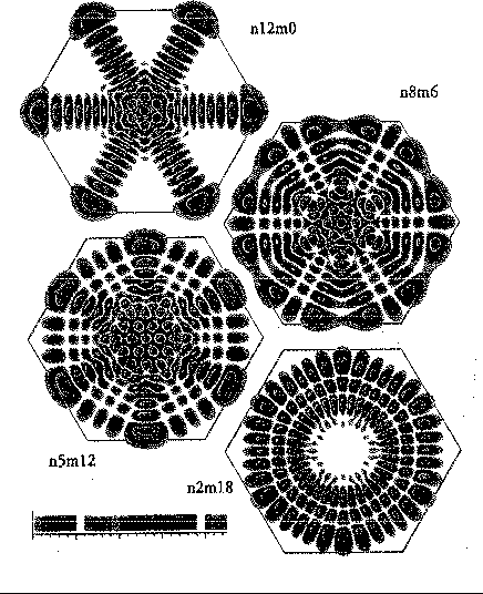
Quantum variational methods are quite useful here too since we cannot solve the quantum problem exactly, either for the ground state or excited states. To describe the symmetry species of the symmetry group C6v of the quantum Hamiltonian we can use eigenfunctions of the 2D isotropic harmonic oscillator [44]. In polar coordinates these are products of an exponential times a function of ( or ) times times a Laguerre polynomial in times a normalization factor. Although the azimutal quantum number is not conserved with the Hamiltonian (4.25) it is conserved modulo 6 due to the hexagonal symmetry of the problem. We can as a first approximation minimize the diagonal elements of the Hamiltonian (4.26) in this basis with respect to the frequency and obtain first order estimates for the energies of states which are labelled by a principal quantum number n and m(modulo 6). For example the energy of the ground state (n,m)=(0,0) is overestimated by about in this basis while energy of the state (n,m)=(15,0) is overestimated by about . “Exact” energies can be obtained by diagonalizing the Hamiltonian in a large basis of harmonic oscillator states and minimizing eigenvalues with respect to . Another variational procedure uses products of Airy functions along the groove and perpendicular to it, and takes the scale factors of the two Airy functions as variational parameters. For the excited state (15,0) the error is (the “exact” energy is 16.34869 while the Airy approximation gives 16.3511). More examples can be found in Table 1 of reference [41] . The probability densities of a few states are shown in Fig. 4 where one can see one low angular momentum state (12,0) and one high angular momentum state (2,18) and two states which presumably correspond to chaotic trajectories.
4.3 He Atom Inside C70 Cage
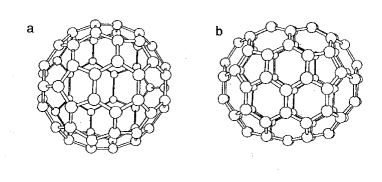
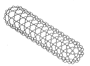
Endohedral fullerene complexes such as He @ C70 have attracted much study in recent years, both experimental and theoretical (for reviews see [45, 46, 47, 48, 49]). Here X @ Cn denotes species X (atom, ion or molecule) encapsulated in a Cn cage [50]. Early theoretical work focussed on the prediction of infrared and Raman [53, 54] and neutron scattering [49] spectra due to the motion of X = He, Li+, Na+, K+ and CO inside the near-spherical C60 cage. The predictions of [53] were subsequently confirmed experimentally [55, 56] for the infrared bands of Li+@C60. Confirmation of the predicted Raman bands [53] of Li+@C60 is tentative [56]. Later the theoretical studies were extended to study the dynamics and spectra of atoms, molecules and ions trapped in nonspherical cages, e.g. He @ C70 [57, 58, 59], Ne @ C70 [60], He @ C250 (nanotube) [61], Na+ @ C120 (nanotube) [62], and even (C60)n @ C∞(nanotube), so-called nanopeapods [63]. Figs 5 and 6 show C60, C70 and carbon nanotube cages.
The C60 cage, assumed to be rigid, presents a very nearly spherical potential [64] for an entrapped atom or ion X and the dynamics has been studied by various classical [66], semiclassical [48] and quantum [48] methods. The potential can be calculated by a variety of semiemperical and ab initio methods [47, 48, 66, 67]. The dynamics is usually quite regular [64] for X@C60. We discuss here instead the case He @ C70, where the potential is highly non-spherical and gives rise to nonintegrable (chaotic) dynamics of the He atom [57, 58, 59]. We estimate the energy levels semiclassically [58, 59] using the UMP as described earlier, and compare with the “exact” results obtained by brute-force diagonalization of the Hamiltonian [57]. Classical simulations of the motion have also been carried out [57, 58, 59], and provide insight as to the degree of chaos in the motion of the He atom. The chaos is surprisingly small, given that the potential is strongly anharmonic. The small degree of chaos implies an approximate third constant of the motion [68], in addition to the energy and -component of angular momentum (assuming the potential is axial).
The potential for He in a rigid C70 cage has been estimated semiemperically [57], and, to a good approximation, is axially symmetric around long -axis in Fig 5b . With origin at the centre of the cage and axes perpendicular to the symmetry -axis, the potential has been fit to the form
The first two terms describe a 3D anisotropic harmonic oscillator, with frequencies and , where is the He atom mass. We use the standard spectroscopic unit () for frequency and energy (see [58]). The last term in (4.27) is a quartic perturbation, with when are in units of . There are also smaller terms in (4.27) varying as , , etc, which we shall ignore.
Because of the axial symmetry we change to cylindrical polar coordinates ( and write the Hamiltonian, with potential (4.27), as
where , and is the z-component of the angular momentum, which is a constant of the motion. The cage has been assumed to be rigid and fixed in space. To apply the UMP (2.10), we proceed exactly as for the simpler spherical pendulum example of sec.3.2. When viewed down the axis, the trajectory is roughly a precessing ellipse, and the -motion is oscillatory. We therefore take as a trial trajectory
where the axes precess with some (unknown) frequency with respect to , and where may differ from , etc. Calculating and with the trial trajectory and applying the UMP gives to first order in (see [58] for the details) , the shifted frequencies
and also, to first-order in , as a function of the partial actions
The terms of second-order in in (4.30) and (4.31) are also derived in [58], and it is also found that to second order. The simulations show that is small but nonzero in general, and to obtain from the UMP requires an improved trial trajectory over (4.29), e.g. one involving higher harmonics of and [59]. We shall ignore this small effect here.
To estimate the energy levels semiclassically from (4.31) is very simple: according to the EBK quantization rule (2.11), we replace by , etc. This gives
where the and terms are written down in ref. [58]. We compare the semiclassical energy levels (4.32) (including the and terms) with the fully quantum results; the lowest 613 levels, up to the energy of are obtained by diagonalizing the Hamiltonian in a harmonic oscillator basis in [58]. The harmonic oscillator chosen has a potential given by the harmonic part of (4.28). The semiclassical and fully quantum results agree to better than . We illustrate the good agreement in Fig 7, which shows the levels up to , organized according to , the quantum number corresponding to .
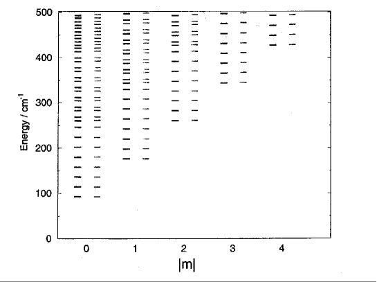
For an isotropic 2D harmonic oscillator, the energy depends only on . For , for example, we can have , which are degenerate. The -values allowed for are . For general , we have or . For our oscillator (4.28) the different states should in reality have different energies; this is found in the fully quantum calculation, but not in the semiclassical one where the energy depends only on . Table 2 illustrates more clearly the slight splittings found quantum mechanically, but not semiclassically.
To obtain the splittings semiclassically requires an improved trial trajectory over (4.29), one that gives a nonvanishing precession frequency . This is discussed in ref [59]. The simple improvement in the trial trajectory mentioned earlier (including some higher harmonics) does indeed give a nonvanishing and hence splitting. However the trial trajectories employed thus far are unable to give accurate splittings, and hence require further improvement.
Table 2
| 0 | 2 | 2 | 262.818 | 263.466 |
| 0 | 2 | 0 | 262.821 | 263.466 |
| 1 | 2 | 2 | 284.696 | 285.403 |
| 1 | 2 | 0 | 284.699 | 285.403 |
| 2 | 2 | 2 | 306.574 | 307.340 |
| 2 | 2 | 0 | 306.577 | 307.340 |
Comparison of selected energy levels calculated via quantum and semiclassical methods demonstrating the failure of the simple variational calculation to produce level splitting observed in the quantum results.(from ref.[58])
5 Nonconservative Systems
In this section we consider nonconservative mechanical systems. For example consider a system of particles moving in the time-dependent external field, or a system whose parameters depend explicitly on time. Other examples include time-dependent constraints, e.g. a bead on a rotating hoop whose angular velocity is a prescribed function of time, and variable mass systems (for which in general [69]). Such systems are not closed and the energy is not conserved. The evolution of a nonconservative system is completely determined by a time-dependent Lagrangian or by a time-dependent Hamiltonian . (We exclude dissipative systems from our discussion. We do note that Lagrangians and Hamiltonians have been found for such systems in some cases [70], so that the action principles discussed here would apply in these cases. Alternatively [5], dissipative terms can be added to the Lagrange equations of motion or to the Hamilton principle.) and are related to each other by the Legendre transformation (see eq. (2.5))
Locally these lead to the usual Euler-Lagrange or Hamilton equations of motion that govern the dynamics of the system.
5.1 Action Principles
We consider the global description of nonconservative systems. It is well known that the Hamilton Principle
is applicable for nonconservative systems as well as for conservative ones. Here subscript reminds us that variations near the actual path are constrained by fixing the travel time from the initial point to the final point . Again we have chosen and , and, as before, it is understood here and below that the end-positions and are also fixed.
As before, we can relax the constraint of fixed and rewrite (5.2)[12, 71] as an unconstrained Hamilton Principle (UHP)
where the Lagrange multiplier is the true value of the energy at the time of arrival at the final point . (Elsewhere in this paper is denoted variously as , or ; see notes [25] and [73]). We assume that all trial trajectories start at the same time and also have the same end positions and .
Using eq.(2.7), which is derived from (5.1) as before, we transform the UHP (5.3) to the form
This is the unconstrained Maupertuis Principle (UMP) for nonconservative systems, which seems not to have been given in the literature explicitly (it is implicit in an Appendix in [12] - see also [73]). It relates three variations - the variation of mean energy , the variation of the action and the variation of the travel time . The Lagrange multipliers are the true travel time and the difference of energy and mean energy of the true trajectory at the final point, . The latter can be rewritten as
where the bar and brackets both denote a time average over the interval (0,T). The generalized UMP (5.4) can also be derived by traditional variational procedures ([12], eq.(A.6)).
One can derive constrained principles from (5.4) as before, e.g. , but these would be complicated to use in practice because of the severe constraints on the trial trajectories. The version is closest to the original Maupertuis Principle. The constrained principle
is mentioned by Whittaker [75], and is easily derived from (5.4) and (5.5). But since (5.4) is also valid without fixing and , (5.4) is more convenient.
Formally the unconstrained Maupertuis principle (5.4) is equivalent to the Hamilton principle, but it also appears too complicated to be useful in practice. This is not quite true and we demonstrate how the UMP can be used for adiabatic perturbations.
5.2 Adiabatic Invariants and the Hannay Angle
For simplicity we start with a one-dimensional periodic system that depends on a parameter . Let vary with time adiabatically, i.e. the change during a period of oscillation . It is well known that in this case the energy as well as the period of oscillation depend slightly on time, but the action over a cycle, where
remains constant to an excellent approximation (adiabatic invariant) when the parameter varies.
Consider what kind of information can be extracted from the UMP (5.4). Both the energy and the period of an actual motion are functions of the action (recall the action-angle variables): , . Consider two actual trajectories with actions and as two trial trajectories for the UMP (5.4). Then the variational equation can be rewritten as a differential equation
It is more convenient to rewrite this in terms of the frequency ,
This equation generalizes the standard relation [5] for integrable conservative systems
to integrable nonconservative systems.
Up to this point (5.7) and (5.8) are general and valid for any nonconservative system for which a good action can be defined. Consider now the adiabatic regime where the variation of the parameter over the short period , , is much less than the parameter itself: . In this case
where the averaging is to be performed at a fixed value of since varies little over a period . The action is conserved for any given parameter , and hence the derivative is also a constant of the motion. As a result in this approximation we get
In the same approximation we have for in (5.8)
Thus to the first order approximation in we can rewrite (5.8) as
or finally as
Here is the zero-order term, and is the variation of the parameter during the given period. We get corrections (of the first-order in the nonadiabaticity parameter ) to the frequency of oscillation, for adiabatic systems. The result seems very simple. It appears that is a continuous function of time and we calculate some average frequency over the period. But actually is not always a continuous function of time; it is a global parameter of a (slightly) aperiodic system. Thus (5.10) is nontrivial in general.
To illustrate these results it is instructive to consider a simple exactly solvable example. We consider the 1D motion of a perfectly elastic ball of mass bouncing between two planes. We suppose that one plane is fixed and the other is slowly moving with constant velocity . We suppose also that the planes are heavy enough so that they are unaffected by collisions with the ball. The distance between the two planes is the adiabatic parameter.
Let us define a cycle as the motion of the ball from the fixed plane to the moving plane, collision, and the motion of the ball in the backward direction up to the collision with the fixed plane. The n- cycle can be described in the following way. At time (beginning of the cycle) the ball has velocity , and the distance between planes is . At time the ball collides with the moving plane and after the collision it moves to the fixed plane with velocity (the collision with the fixed plane is elastic and the backward velocity is equal to the forward velocity after collision, i.e. ). The backward motion takes time . The period of the whole cycle is . At time (the initial time for (n+1)-th cycle) the distance between the two planes is equal to . This means that is an exact (adiabatic) invariant.
It easy to see that the action is proportional to this invariant,
i.e. the action is an exact (adiabatic) invariant for our special initial condition [74].
In terms of the action and the adiabatic parameter the complete set of relevant quantities is as follows:
i.e. is linear function of the nonadiabaticity parameter and the approximate relation (5.10) must be exact here. Indeed, we have , and
Thus the approximate relation (5.10) is valid here. It is also not difficult to check after a little algebra that in the exact relation (5.8) all higher powers of cancel each other and the linear approximation is exact.
If is not extremely small, ceases to be an adiabatic invariant and the system becomes nonintegrable. If is varied nonadiabatically and periodically around , the system (termed the Fermi model [76]) can show steady energy growth and chaotic motion.
The generalization of (5.10) to multidimensional integrable systems with actions ,…, is evident, as is the generalization to multiparameter systems, with parameters .
The corrections in have been derived by other methods [77], but in different forms from (5.10). If we assume is periodic, with a long period , the terms in , when integrated over , define the Hannay angle , the classical analogue of the quantum Berry phase [77]. The Hannay angle is the extra (geometric) phase undergone by the system in one cycle of , in addition to the more obvious dynamical phase obtained by integrating the instantaneous frequency . In general one requires more than one -type parameter to obtain a nonvanishing result for , but Hannay and Berry and coworkers give a few examples [77, 78, 79] where one parameter suffices. We discuss two examples with nonvanishing .
5.2.1 Bead Sliding on Slowly Rotating Horizontal Ring
Consider a bead of mass sliding without friction on a closed planar wire loop which is slowly rotating with angular velocity in the horizontal plane. For a loop of arbitrary shape, Hannay and Berry [77] show that the Hannay angle defined above is given by , where is the area and the perimeter of the loop. For a circular loop rotating about an axis perpendicular to the plane of the loop and through the center, is simply , as is clear intuitively: the “starting line” for the particle moves ahead by while the particle rapidly slides around the loop.

We consider a circular loop of radius (Fig.8), but with the vertical axis of rotation through a point on the wire instead of the center of the loop, to make the answer less obvious. The adiabatic parameter here is the prescribed orientation of the loop , where is small. We do not at this stage assume is constant.
Using the horizontal lab-frame (Fig.8), we can easily write the Lagrangian, which is just the lab kinetic energy of the particle. Using in Fig.8 as the generalized coordinate we find
From (5.11) we obtain the equation of motion
If the loop rotates uniformly (), (5.12) is just the pendulum equation, as one expects intuitively.
Because we are using a rotating coordinate system ( is measured from ) is not equal to in this system, so that the Hamiltonian is not equal to the energy () in this system either. To find , we first calculate the canonical momentum , where
and then is
In terms of the canonical variables , the Hamiltonian is
where we drop terms since we assume .
We cannot apply (5.10) as it stands, since was used in the derivation. The generalization to include cases where is
where is the average of over the fast motion (here ). Alternatively, we can use (5.10), with now . From (5.15) we have
since varies rapidly and is nearly constant.
We now assume is constant. For , is a function of the good action only (no dependence), and when we see remains a good action. Note that is independent of angle , so that the second term in (5.16) will not contribute to , which is
The total phase undergone after a long return time is thus
The first term is the dynamical phase, the second is the Hannay (geometric) phase.
5.2.2 The Foucault Pendulum
For a Foucault pendulum the Hannay angle is the angle by which the plane of the pendulum vibration shifts in one day, i.e. , where is the co-latitude of the point on earth where the pendulum is located. This is a clockwise rotation in the northern hemisphere. This result for has been derived by Berry [79] and others [80] by various arguments. There are also some pre-Hannay purely geometric arguments for the Foucault pendulum precession [81]. Here we show the result follows simply from (5.16).
We consider a pendulum of length and bob mass oscillating at a point on the earth’s surface with co-latitude . We use axes x,y,z attached to the earth, with x,y in the horizontal plane and z vertical. When at rest in the x,y,z system, the pendulum hangs along the z-axis, and when in motion the bob oscillates very nearly in the x,y plane. Neglecting the z motion and assuming is small, where is the earth’s angular velocity, we easily find [82] the approximate horizontal equations of motion
where . We have kept the Coriolis terms, but dropped the centrifugal terms, since is small compared to the pendulum frequency . Here is the local vertical component of the earth’s angular velocity. We are interested in particular in the orbit precession rate predicted by (5.20).
It is easily checked that (5.20) follow from the Lagrangian
and of course (5.21) can be derived directly [83].
Changing to polar coordinates , via , changes to the form
Two constants of the motion are obvious from (5.22): since does not depend on , is a constant, where
and because does not depend on explicitly, the Hamiltonian is a constant, where and
Two constants of the motion with two degrees of freedom imply that the system is integrable and that two good actions exist.
To express in terms of the canonical variables , , , we use (5.23) and
to get
where again we drop an term. We wish to use (5.16) (not (5.10) here as ) to find the frequencies and , where is the orientational angle of the earth multiplied by . Note that for , (5.26) is simply the Hamiltonian for an isotropic 2D harmonic oscillator. Calculation of the actions for the 2D oscillator, and , is a standard exercise [84], and the Hamiltonian in terms of these actions is
The term in (5.26) will not disturb the good actions, so that (5.26) becomes
Application of (5.16) with and then gives
where a positive (+) frequency in corresponds to a counterclockwise rotation. Note that the Foucault precession frequency is true for orbits of any shape, e.g. near linear (the usual case), elliptical, or circular. The factor of 2 in in (5.29) is clear intuitively: for , in one circuit of an elliptical orbit, goes through two cycles while goes through one. Computing the phase of the pendulum after one complete rotation of the earth (period ) then gives
The term is the dynamical phase and is the geometric Hannay angle .
The examples in this section and the previous one led to a nonvanishing Hannay angle . It is easy to show that the earlier example (particle in a 1D box with a slowly moving wall) gives a vanishing result. The same is true for a particle in a slowly rotating 1D box (fixed walls). Golin [85] has proved that, for 1D systems with one adiabatic parameter , one always has unless undergoes a rotational excursion through . However the proof does not cover our rotating 1D box example (which has a hard wall potential), since Golin [85] assumes a smooth potential. The case of a slowly rotating 2D box of elliptical shape has been worked out by Koiller [80], and gives a nonvanishing depending in a complicated way on the area of the box.
5.2.3 Nonintegrable Systems
Nonintegrable systems have fewer than independent constants of the motion or good actions, where is the number of degrees of freedom. For such systems, at least some of the possible motions are chaotic, and for these at least some of the good action variables do not exist. Hence we have not been able to proceed rigorously beyond the general relation (5.4) for chaotic motions. (Despite the nonexistence of good actions for nonintegrable systems, formal use of them and their adiabatic invariance have been used successfully in semiclassical quantization schemes; see sections 2.3, 3.1, 4.1, 4.3 and ref. [13] for a method based on the Maupertuis Principles for conservative systems, and see refs. [91, 92] for a method based on adiabatic switching.)
As stated, we do not have rigorous arguments to draw consequences from the UMP (5.4) for nonintegrable systems, but some heuristic arguments can be given. For example, by choosing to vary slowly and linearly with , e.g. , where is small, we can derive the adiabatic invariance of the action for a 1D periodic system (earlier we assumed that is an adiabatic invariant for such systems). Further, by considering long trajectories of multidimensional systems, which start and end in some small region in phase space, and which are not quite periodic in general, we can formally show that, in a Poincaré cycle time or in the limit the long-path action is an adiabatic invariant for quasiperiodic and chaotic trajectories of multidimensional systems. Ehrenfest [95] has previously shown that is an adiabatic invariant for multidimensional periodic systems. For ergodic systems, the phase volume is an adiabatic invariant (see next paragraph), and since the adiabatic invariant is apparently unique for such systems (Kasuga [90]), it should be possible to derive the adiabatic invariance of from that of for these systems, but we have been so far unable to do this [86]. We note that counterparts of the Hannay angle have been established for adiabatically evolving nonintegrable [88] and ergodic [89] systems.
For one limiting case, complete chaos (ergodic motion) where the energy is the only constant of the motion, and long trajectories typically cover essentially the whole energy surface, a rigorous adiabatic invariant has been found [90, 91, 93], i.e. the phase volume , enclosed by the energy surface :
where is the step function, which is unity for positive argument. (For multidimensional systems, stands for .)
If depends on a slowly varying parameter so that , then . The adiabatic invariance of is intuitively plausible [94]. First consider the initial () energy surface , and its image under an arbitrary time development (i.e.not necessarily slow). The final (image) surface at the time is not in general a constant energy surface, and hence not in general a dynamical surface. However, by Liouville’s theorem the volume enclosed by the final surface is equal to that enclosed by the initial surface. If the time-development from to is sufficiently slow then at each stage the surface which has evolved from the surface is a dynamical surface, by definition of adiabatic evolution, where allowed motions transform into allowed motions [95]. In this case the final surface is a true constant energy dynamical surface, and hence from Liouville’s theorem .
For ergodic systems, there are no good quantum numbers except for the energy-ordering quantum number , where . A rough but useful semiclassical quantization scheme for ergodic systems based on is the Weyl rule [93]
which implicitly defines . This is just a restatement of the early rule due to Planck [96] that each quantum state occupies a volume of size in classical phase space. In practice, various improvements such as replacing by as in (2.4) are used [93]. More subtle improvements can be obtained from Gutzwiller’s trace formula [28]. These relate fluctuations from the smooth dependence of on predicted by (5.32) to the classical periodic orbits. In cases such as the potential, where the classical diverges [98] due to the infinite channels of the potential (see Fig.1), one can estimate the smooth part of ( the cumulative number of states up to ) quantum mechanically [97] at low energy by an asymptotic expansion [98], with leading terms and , where is dimensionless. Application of the generalization of (5.32), i.e. , then gives reasonable estimates of the low-lying state energies [36, 98].
5.3 The Classical Hellmann - Feynman Theorem
Another consequence of the UMP (5.4) is the classical version of the Hellmann - Feynman theorem [99]
Here depends on a parameter , so that the energy depends on , as well as on the (constant) action , and denotes a time-average over a period at fixed action . We assume a one-dimensional periodic system for simplicity.
The quantum version of the theorem [100] is nowadays much better known, i.e.
where , and where the Hamiltonian operator depends on some parameter , so that the energy eigenvalue and eigenfunction do also, because of
Proof of (5.34) is simple; we apply to both sides of the relation , and note that the two terms involving add to zero because of (5.35), the hermiticity of , and the fact that we assume for all .
It is clear that (5.33) is the classical limit of (5.34), since as (or ) approaches a time average over a period, and fixing corresponds to fixing , since . To derive (5.33) from (5.4) we consider to evolve adiabatically, so that and in (5.4) can be related. The derivation is intricate, however, and it is simpler to proceed instead from the RMP (2.3) for conservative systems. We apply (2.3) to two periodic trajectories of , the true one with period , and a virtual one taken as the true trajectory of with period . Since first-order variations in vanish (at fixed ), we have
where is an average over the trajectory with period , and it is understood that is the same for both and . From (5.36) we get for to accuracy
Again neglecting terms we have
Eq(5.37) yields , and since for the true trajectory we get , the Hellmann-Feynman relation (5.33) apart from notation.
As a simple example of (5.33) consider a 1D harmonic oscillator, with Hamiltonian and , where is the angular frequency. Choose , the force constant. The left side of (5.33) is and the right side is . Thus we have , as is well known from the virial theorem [5]. If we choose , we find similarly .
As a second example, consider the bound motion of a 1D system with Hamiltonian . We change variables via the transformation , , where is an arbitrary scale factor. This transformation is canonical and preserves the Hamiltonian [101], i.e. , where
The energy of a given state of motion is unchanged by the change from to for any value of . We now use (5.38) in the Hellmann-Feynman relation (5.33). The left hand side vanishes. The right hand side derivative is
where , and we have reverted to the original variables in the second form. Hence we get
i.e. the virial theorem for an arbitrary potential .
6 Variational Principles in Relativistic Mechanics
Hamilton’s Principle is widely used in Classical Relativistic Mechanics and in the Classical Theory of Electromagnetic and Gravitational Fields to derive covariant equations of motion (see, e.g.[102]). As for Maupertuis’ Principle, it is widely believed that it is not well suited for that purpose because when operating with the energy one loses explicit covariance. In this section we demonstrate, first, how to use Maupertuis’ Principle for the derivation of the covariant equations of motion and, the second, how to use it for the solution of specific problems.
Consider a relativistic particle with mass and charge moving in an arbitrary external electromagnetic field, described by a four-potential with contravariant components , and covariant components , where and (for ) are the usual scalar and vector potentials. Hamilton’s Action for this system can be written in the Lorentz invariant form [102, 103]
where we use the sign of Lanczos [103] for , opposite to that of Landau and Lifshitz [102]. The sign can be chosen arbitrarily; our choice allows us to use below the orthodox definitions and . The four-dimensional path runs from the initial point to the final point in four-dimensional space-time with corresponding proper times and . Here is the infinitesimal interval of the path (or of the proper time) , the metric has signature and we use the summation convention and units with , where is the velocity of light. is itself not gauge invariant, but a gauge transformation ( for arbitrary ) adds only constant boundary points terms to , so that is unchanged. The HP is thus gauge invariant.
If we introduce a parameter along the four-dimensional path (proper time along the true or any particular virtual path are valid choices) the action can be rewritten in the form
where . In general, is both frame-independent and path-independent. A path-independent parameter is here invaluable for variational purposes, since we then do not have to vary the parameter when we vary the path. After the variations have been performed, we can then choose , etc. The limits of the integrals are the invariants and . With respect to parameter we get the covariant Lagrangian
and corresponding conjugate momenta
and Hamiltonian
Thus in this particular covariant treatment the Hamiltonian is trivial. The dynamics is hidden in a constraint. One can see that the four conjugate momenta are not independent variables but satisfy the constraint
which is obvious from (6.4). This constraint can be taken into account with the help of the Lagrange multiplier method, i.e. with the help of an effective Hamiltonian [103, 108]
We easily find that the Hamilton equations of motion with are equivalent to
(for , the true trajectory proper time ) and to the covariant Lorentz equations of motion for a charged particle in an external field:
i.e. the same equations as are found from the Lagrangian (6.3) (see, e.g. [102]).
On the other hand the Hamilton equations with are equivalent to the MP or to the RMP with the same . Thus one can use any of the four Variational Principles (HP, RHP, GMP, RMP) either with Lagrangian (6.3) or with effective Hamiltonian (6.7) for the derivation of the covariant equations of motion. It is to be noted that in the covariant formulation of relativistic mechanics, the Hamiltonian (a Lorentz scalar) is not equal to the energy ( the time component of a four-vector). Thus in the Maupertuis Principle must be interpreted as
where . By contrast, in the noncovariant formulation discussed below, the Hamiltonian is equal to the energy .
There are other, related, formal difficulties arising from (6.5). This condition () is due to the fact that the Lagrangian in (6.3) is homogeneous and of first degree in (i.e. essentially linear in velocities ), so that and hence the difference (the Hamiltonian) vanishes [104]. Since , the Legendre transform relation (6.5) between and simplifies to
and hence the Legendre transform relation between and , i.e. (where ), simplifies to
Because , direct application of the GMP ( would be cumbersome, and direct application of the RMP ( would be impossible.
All these difficulties can be traced to the well studied difficulty [5, 103, 105, 106, 107] of applying an action principle with kinematic [109] nonholonomic constraints, such as (6.6) for the momenta, or for the velocities for proper time , or for arbitrary parameter .
One way out of the difficulties is to introduce the constraint with a Lagrange multiplier for either the Lagrangian or Hamiltonian (as is done above for ). Another way out is to exploit the nonuniqueness of the Lagrangian. For example [105], the covariant Lagrangian (6.3) is equivalent to the covariant Lagrangian , where (with as parameter)
where . It is easily verified that (6.12) generates the same Euler-Lagrange equations of motion as (6.3). For (the proper time of the path in question), (6.12) simplifies to
which is often employed [5, 106]. The advantage of (6.12) and (6.13) is that they are nonhomogeneous in , and hence will generate a nontrivial corresponding Hamiltonian . For (6.13), for example, we find
Note that (6.14) and (6.7) (for ) differ only by a constant. Use of the covariant and in place of and removes the difficulties of using all four variational principles (HP, RHP, GMP, RMP). For and , only the first two can be used. Note again that is computed from as in (6.9), with in place of .
Now we come to the question of the solution of specific physical problems. In this case explicit covariance usually is not of great importance and it is more useful to find an appropriate convenient frame. For any given frame we can choose (the coordinate time) and obtain the complete set of nontrivial quantities
The expression for in (6.15) is derived from (6.3) or (6.12) by choosing , except that we have used the freedom to change the sign of to agree with the standard choice in the noncovariant case [5]. Again we have chosen and . Note that the nonrelativistic form for the Maupertius action is not valid here, and also note that the Hamiltonian is equal to the energy , despite the fact that .
As a result the complete set of four variational principles is available in any particular frame. It is matter of taste or practical convenience to use one principle or another. From a practical point of view there is no difference in the usage of variational principles in nonrelativistic mechanics and in relativistic mechanics in a given frame.
As an example of the usage of the GMP for relativistic mechanics consider the motion of an electron in a uniform magnetic field . A corresponding vector potential in the Coulomb gauge () is , or [116]. The solution of (6.8) in this case is well known - the electron moves with constant velocity along the direction of the field (along the z-axis in our case) and along a circular orbit in the plane with the cyclotron frequency
where is the total energy of the particle including the kinetic energy of the motion in the z -direction.
To calculate this frequency from the GMP we take as a trial trajectory
where and are free parameters. After some simple algebra we get
In this case it seems that an economical method is to use the GMP (2.2). For this purpose one has to rewrite as a function of
and to calculate the variation at fixed . The GMP (2.2) translates here to . One then easily finds the analytical solution
The exact solution corresponds to the case when . For our trial trajectory, we happen to have and the approximate solution coincides with the exact one ( similar to the case of a harmonic oscillator).
This simple example demonstrates how to use variational principles for relativistic systems.
7 Classical Limit of Quantum Variational Principles
In section 2.1 we mentioned that the classical limit of the Schrödinger Quantum Variational Principle is the Reciprocal Maupertuis Principle for periodic or other steady-state motions, i.e.
where is the Hamiltonian operator corresponding to the classical Hamiltonian . Here is the period for periodic motions, or for other steady-state motions (quasiperiodic or chaotic). Solution of the left-hand side yields [118] the stationary state with the energy eigenvalue , i.e.
the time-independent Schrödinger equation. Details of the proof of (7.1) (which is straightforward only for integrable systems) are given in [12]. In ref.[119] it is explained how Schrödinger, in his first paper on wave mechanics in 1926, in essence worked backwards, i.e. starting from the right hand side of (7.1), he “derived” the left hand side, and thereby discovered wave mechanics. In his second paper on wave mechanics in 1926 he retracted this argument because his version of the right hand side of (7.1) was not quite correct. In this second paper he presented an alternative argument as a basis for wave mechanics (now in the standard textbooks) based on the analogy between geometric and wave optics on the one hand, and particle and wave mechanics on the other.
We consider now the generalization of (7.1) to nonstationary states , where the true dynamical states satisfy the time-dependent Schrödinger equation
where , and the initial state is given. For notational simplicity we consider a single particle in three dimensions, so that , and
where and = . The arguments which follow are also valid for nonconservative systems, where .
We shall consider here the quantum time-dependent variational principle due to Frenkel and Dirac [120, 121, 122] for the wave function , but we note the existence of other quantum time-dependent variational principles, e.g. for the time-evolution operator and transition amplitudes [123], for the Heisenberg operator version [124] and for the matrix mechanics version [125] of the Hamilton Principle, for the density matrix [126], for the mean value of an arbitrary observable [127], and for time-dependent density functional theory [128]. ( For completeness, we note that there are also other [130] quantum time-independent variational principles, in addition to that of Schrödinger.)
The original Frenkel-Dirac variational principle is [120]
for arbitrary variations around the true dynamical state . Since (7.5) is true for all possible variations , then for the true states, as in (7.3). By adding (7.5) and its complex conjugate and using the hermiticity of we can transform (7.5) to [129]
Integrating over an arbitrary but fixed time interval , and assuming is fixed, we find [131] from (7.6)
Note that (7.7) is not in the traditional form for a variational principle , because of the right hand side. It is more like the unconstrained principles discussed earlier. Some authors drop the right hand side without comment [132], but it is required if arbitrary variations in are allowed; otherwise (7.7) will not generate the Schrödinger equation (7.3) and its complex conjugate [129]. It is possible to obtain a vanishing right-hand side by restricting the variations in various ways [133], e.g. requiring the trial wave functions to be normalized at all times. Another way is to write the right hand side as , formally regard and its complex conjugate as independent (see below), and assume (as well as ) is fixed. However, we find it simplest to retain the general form (7.7), with no constraints on except for the fixing of the initial condition . (When dealing explicitly with bound states later, we assume boundary conditions on .)
By writing out the scalar products in (7.7) and using the hermiticity of , we can write (7.7) in field theory form
where the Lagrangian density is
Since is a complex function, whose real and imaginary parts can be varied independently, it is well known [134] that and can be regarded as independent for variational purposes. These two variations in (7.8) with given by (7.9) will generate the Schrödinger equation and its complex conjugate.
Following Feynman [132], we change variables (or ) in the Lagrangian density , where is the amplitude and the phase of the wave function, via the Madelung transformation [135]:
where is the probability density. In terms of and we have
In terms of the boundary term in (7.8) is
We now take the classical () limit of (7.8). Using (7.11) and (7.12) we get
We have assumed that in the limit , and approach well defined limits ( which we continue to denote by and ). In particular we assume that does not contain an term [136]. We vary and independently in (7.13). Varying , with fixed, gives
Since is arbitrary, the bracket […] must vanish, so that
This is the classical Hamilton-Jacobi equation [138] for the classical action along true paths.
Next we vary in (7.13) with fixed. We integrate the term by parts using
where we drop a surface term by assuming for . This assumes the corresponding quantum state has finite norm. We integrate the term by parts using
where we use which follows from the fixing of . Using (7.15) and (7.16) in (7.13) thus gives
Since this is true for arbitrary , we get
This is the continuity equation, reflecting conservation of total probability, since [138] is the momentum of the particle. Note that if the right hand side of (7.13) were missing, we would not get the correct continuity equation. In contrast to what we have done here, Feynman [132] keeps the terms in (7.11), and the variational principle then leads to quantum generalizations [137] of the Hamilton - Jacobi (7.14) and continuity (7.17) equations.
Thus we see that the classical limit of the quantum time-dependent variational principle is the classical variational principle for the Hamilton-Jacobi and continuity equations. Interestingly the classical limit of the quantum time-dependent variational principle leads to a classical variational principle for the Hamilton action along the true trajectories, whereas the classical limit of the quantum time-independent variational principle in the form of the left side of (7.1) leads to a classical variational principle for the trajectories themselves (RMP -the right side of (7.1)). An alternative form [139] of the quantum time-independent variational principle,
will generate in the classical limit a variational principle for the Maupertuis (or time-independent) action along the true paths. In (7.18) is a constant Lagrange multiplier introduced to remove the normalization constraint . The extremizing ’s which satisfy (7.18) obey
so that is the energy eigenvalue corresponding to the eigenfunction .
To derive the classical limit of (7.18) we proceed much as before. (We assume is time-independent in this section.) We first apply the Madelung transformation to , i.e.
where is the amplitude and the phase. Following similar steps as above, we find (7.18) becomes in the classical () limit
where .
Varying in (7.21) with fixed gives
the time-independent Hamilton-Jacobi equation [138] for the Maupertuis action along true paths. If we vary in (7.21) with fixed we get the continuity equation
since [138] is the momentum of the particle.
In ref.[12], we show how the classical limit of (7.18) can be taken in a different way (using standard 1D WKB wave functions) and for a 1D periodic orbit leads to , i.e. the UHP for a periodic orbit of period .
We note that, just as for the right hand side of (7.1), the derivation of the classical limits (7.14) and (7.22) is somewhat formal for the chaotic motions of nonintegrable systems, since classical values of and may not exist as well defined functions for such systems. Unlike the nonrelativistic limit (), which is regular, the limit or is singular, which makes the classical limit subtle and interesting [140].
8 Summary and Conclusions
We summarize the two groups of classical variational principles reviewed in this paper. First we have the Maupertuis principles:
The first of these is the unconstrained form (UMP), the second the general Maupertuis principle (GMP), and the third is the reciprocal Maupertuis principle (RMP). By Legendre transformation of the principles in (8.1) we obtain the Hamilton principles:
The first is the unconstrained form (UHP), the second the Hamilton principle (HP), and the third the reciprocal Hamilton principle (RHP). In all these principles, the end-positions of the trajectory and are held fixed, and the notation indicates what else is fixed and what is varied.
We have given a number of examples showing how to use these principles to solve practical problems, focussing particularly on the three Maupertuis principles. Both classical and semiclassical applications have been given, and some comparisons are made with the results from quantum variational principle calculations. The classical limits of two quantum variational principles (time-dependent and time-independent) are given. In particular, the RMP is the classical limit of the Schrödinger time-independent quantum variational principle. The RMP is thereby naturally adapted to semiclassical applications
In the applications, the variational principles ( both classical and quantum) are solved by the direct variational method, where one guesses a trial solution containing adjustable parameters, and adjusts the parameters to satisfy the variational principle. The Euler-Lagrange differential equation is not required in this method. When we choose a simple trial solution, the results can be found simply and analytically.
Using the direct variational method the RMP and UMP have been used to estimate semiclassically the energy levels in several examples. The levels can be expressed in analytical form, and the accuracy is quite acceptable in most cases, even for nonintegrable systems which are usually treated by much more complicated semiclassical methods, e.g. the Gutzwiller trace formula [28], or quantizing the Birkhoff-Gustavson normal form [141]. It would be useful to have comparisons of the results from the Maupertuis Principle-based method with those from the latter two and other methods for a number of specific problems. The methods should be compared for accuracy of results and computational complexity. Some limited comparisons of the Maupertuis Principle and normal form methods have been done for the oscillator of sec. 4.1 in refs. [58, 68], and limited comparisons for this model of results from the Maupertuis Principle and the semiclassical adiabatic methods [35] are presented in Table 1 of sec. 4.1.1, but much more extensive comparisons would be of interest.
Variational principles appeal to various individuals for differing reasons, both aesthetic [142] and practical. We have stressed the utility for classical and semiclassical particle dynamics calculations in this review. Engineers too make heavy use of variational principles in solving practical problems of classical continuum mechanics [143]. On rare occasions variational principles have even led to new laws of physics [144].
9 Acknowledgements
We gratefully acknowledge the Natural Sciences and Engineering Research Council of Canada for financial support of this work. We thank Donald Sprung for a careful reading of the manuscript, David Garfinkle for helpful remarks on relativistic mechanics and Stepan Bulanov for help with TeX.
10 Appendix I. Variational Notation and Reciprocal Principles
“… since is the variation of with kept constant, we could conveniently write it as , in accordance with a convention used in thermodynamics… It is curious that in spite of the obvious need in partial differentiation for precise statement of what is being kept constant, such statement is not embodied in customary notation of pure mathematics, though it is provided in thermodynamics,…”
H.Jeffreys and B.S.Jeffreys
Methods of Mathematical Physics
Cambridge U.P.,1946.
Variational problems ask for the function which makes stationary an integral involving the function and its derivatives. Usually there is a constraint which is fixed. For example, we are to find a function , describing a closed planar curve, of fixed length , which maximizes the area enclosed by the curve . and are functionals of : . For our purpose here, we do not need the precise form of or . is the constraint and is the functional to be varied. We use the following notation to describe this variation
where the constraint is indicated as a subscript on the bracket enclosing the variation of the functional . The variation is first-order in , and is called the first variation when higher-order variations are considered [15] . The constraint is denoted explicitly in (A1.1) because it is the most important, or the one we wish to focus on. There may be other constraints which are left implicit, e.g. that the planar curve pass through a given point (). In this paper we always leave fixed end-position constraints on curves (closed or open) implicit.
The solution of the problem (A1.1) is the function , which satisfies a differential equation, the Euler-Lagrange equation. The reciprocal variational problem has the constraint and the varied functional interchanged. In other words, it is described by the equation
The two equations, (A1.1) and (A1.2), have the same solution . The reciprocal variation is searching for the function which makes stationary (here minimizes) the length of a closed curve with fixed enclosed area . The common solution for both problems is a circle, as is clear intuitively. One way to prove reciprocity is to use a trick, due to Lagrange, called the method of Lagrange multipliers. The problem (A1.1) is first restated in unconstrained form as
where the variations of both and are unconstrained and is an undetermined multiplier. To obtain (A1.2) from (A1.3), we simply specify that we now fix (i.e. set ) and vary , i.e. . This proves the reciprocity theorem.
Reciprocity is clear intuitively in the isoperimetric problem (A1.1). An example of reciprocity from physics is the Gibbs conditions for equilibrium in thermodynamics [117]. The reciprocal conditions and are both conditions for thermal equilibrium, where is the entropy and the internal energy. These express the facts that the state of thermal equilibrium is that state which maximizes the entropy for fixed internal energy, and also is that state which minimizes the internal energy for fixed entropy. (The unconstrained form [145] is , where the Lagrange multiplier is the temperature . Here the implicit constraints in all cases are fixed system volume and mole numbers ) Reciprocal VP’s in mechanics have only recently been studied [12, 13] - see Sec.2.
This is all we shall need from the calculus of variations; for more details one should consult a text-book [146].
11 Appendix II. Equivalence of the Maupertuis and General Maupertuis Principles
In Sec. 2.2, for conservative systems, we discussed the equivalence of the Hamilton Principle (HP)
with the General Maupertuis Principle (GMP)
Here we show directly the equivalence of the GMP (A2.2) with the original Maupertuis Principle (MP)
In all these principles the end-positions and are held fixed. Since (A2.1), (A2.2) and (A2.3) all generate the same (Euler-Lagrange) equations of motion, it is clear they must be equivalent, and it is interesting to show directly the equivalence of (A2.2) and (A2.3). We must show that relaxing the constraint of fixed in (A2.3) to fixed in (A2.2) does not generate spurious or unphysical solutions.
The constraint of fixed in (A2.3) applies along and between the trial trajectories. To relax this constraint, we use the method of Lagrange multipliers [147]. Since , we have , and hence
where is an arbitrary constant. The trajectories all start at at fixed point and end at (which may vary with the trial trajectory) at fixed point . We release the constraint of fixed in (A2.3) and choose such that
where indicates a variation from the true trajectory value and in (A2.4). This can be rewritten as
where , and where we recall that the end-time is not fixed in (A2.3) . Recalling the definition enables us to write (A2.5) as
where we have used the fact that on the true trajectory. Expanding (A2.6) gives
The first and third terms on the right hand side of (A2.7) cancel, since on the true trajectory, as assumed in the MP (A2.3).This means
To see that in (A2.8), we apply (A2.8) to the special case of two true trajectories, with actions and and energies and . For this case (A2.8) reads . Comparison of this with the standard relation [5] gives . Hence we have
which is the unconstrained Maupertuis Principle (UMP) (2.10). Fixing in (A2.9) then gives (A2.2), the GMP.
Thus (A2.2) follows from (A2.3). The converse, the derivation of (A2.3) from (A2.2) is easy; we simply restrict the trial trajectories in (A2.2) to those of fixed energy , since the equations of motion following from (A2.2) imply energy conservation. Hence (A2.2) and (A2.3) are equivalent.
We note once more that conservation of energy is assumed in the original MP (A2.3), whereas it is a consequence of the general MP (A2.2).
References
- [1] Nesbet R K 2003 Variational Principles and Methods In Theoretical Physics and Chemistry (New York: Cambridge U.P.); L.R. Ram-Mohan L R 2002 Finite Element and Boundary Element Applications in Quantum Mechanics (Oxford: Oxford U.P.); Drake G W F 1998 Encyclopedia of Applied Physics (New York: Wiley-VCH) 23 121; Gerjuoy E, Rau A R P and Spruch L 1983 Rev.Mod.Phys. 55 725; Epstein S T 1974 The Variation Method in Quantum Chemistry (New York: Academic). Quantum VP’s for scattering states are reviewed in Adhikari S K 1998 Variational Principles for the Numerical Solution of Scattering Problems (New York: Wiley). Classical VP’s for scattering are discussed in ref. [12].
- [2] For example, in Yourgrau and Mandelstam [9] the notation is reversed. Hamilton himself used the current notation, but, for the actions along true paths, termed and the principal and characteristic functions, respectively.
- [3] There is a recent exception: Papastavridis J G 2002 Analytical Mechanics (New York: Oxford U.P.), p. 1044, where the general Maupertuis principle is discussed. This book contains a masterly and historical account of the various variational principles.
- [4] Arnold V I 1989 Mathematical Methods of Classical Mechanics 2nd edition (New York: Springer Verlag)
- [5] Goldstein H, Poole C and Safko I 2002 Classical Mechanics 3rd edition (New York: Addison Wesley)
- [6] Sommerfeld A 1964 Mechanics translated from the 4th German edition ( New York and London: Academic Press)
- [7] In this review we focus on global (integral) VP’s. We do not discuss the various local (differential) VP’s due to d’Alembert, Gauss, Hertz, Gibbs, Jourdain and others [3, 9, 103]. Jourdain’s principle, and its connections to others, is reviewed by Wang L-S and Pao Y-H 2003 Am. J. Phys 71 72
- [8] For example, Ite U E 2001 Global Thinking and Local Action (Aldershot, Hampshire: Ashgate Publishing)
- [9] Yourgrau W and Mandelstam S 1968 Variational Principles in Dynamics and Quantum Theory 3rd edition (London: Pitman, Philadelphia: W.B.Saunders), reprinted, Dover, New York, 1979; Terral M 2002 The Man Who Flattened the Earth (Chicago: University Of Chicago Press)
- [10] quoted in footnote 77 of Arnold, ref. [4], p 246
- [11] C.G.J.Jacobi 1884 Vorlesungen über Dynamik, zweite ausgabe, herausgegeben von A.Clebsch (Braunschweig/ Wiesbaden: F.Vieweg), reprinted by Chelsea 1969, p 44. The quotation in this text is more explicit than [10]: it names the textbooks of Poisson, Lagrange and Laplace as some of the best!
- [12] Gray C G, Karl G and Novikov V A 1996 Ann. Phys. 251 1
- [13] Gray C G, Karl G and Novikov V A 1996 Am. J. Phys. 64 1177
- [14] Percival I C 1977 Adv. Chem. Phys. 36 1, and references therein
- [15] van Brunt B 2004 The Calculus of Variations (New York: Springer) Ch 10
- [16] Karl G and Novikov V A 1995 Phys. Rev. D 51 5069; 1995 J. Exp. Theor. Phys. 80 783
- [17] Holonomic (coordinate) constraints are assumed to be taken into account by the choice of the . Nonholonomic (velocity) constraints (see note [109]) are assumed absent in the early sections but are considered briefly in sec.6 and App.II.
- [18] We also exclude quasi-coordinates (or nonholonomic coordinates), e.g. for a rigid body, the three rotation angles around space-fixed axes. VP’s using such variables are discussed by Papastavridis [3], and by Marsden J E and Ratiu T S 1994 Introduction to Mechanics and Symmetry (New York: Springer) p 390. A seminal paper is Poincaré H 1901 C.R.Acad.Sci. 132 369
- [19] The condition is valid for normal systems, for which , the holonomic constraints (if any) are time-independent and the reference frame is inertial. If these conditions are satisfied is quadratic in the ’s. Note that the single condition quadratic in the ’s is not sufficient to have since for some systems with time-dependent constraints is quadratic in the ’s: see, e.g. de Castro A S 2000 Eur. J. Phys. 21 23 ; Ferrario C and Passerini A 2002 Eur. J. Phys. 22 11. When , the generalized Maupertuis principles require in place of , where (see Secs. 5.2.1 and 6).
- [20] Percival I C 1974 J. Phys. A 7 794 ; ibid 1979 12 157 ; see also Klein A and Li C-t 1979 J. Math. Phys. 20 572. Percival later extended his VP for invariant tori to cantori: 1980 Amer. Inst. Phys. Conf. Proc. 55 302. A cantorus is, roughly speaking, a torus-shaped surface with holes such that what remains forms a Cantor set of points. A trajectory confined to a torus surface is quasiperiodic. A trajectory starting on a cantorus will slowly “leak away” because of the holes, hence is not confined to the surface so that the quasiperiodicity is destroyed in the long run, and is thus weakly chaotic. See Arnold et al [108], p.194, for a precise definition. Also see Percival I C 1991 in Chaos and Quantum Physics eds. Giannoni M-J, Voros A and Zinn-Justin J 1991 (Amsterdam: North-Holland) p 11
- [21] Greenberg W R, Klein A and Li C-t 1995 Phys. Rev. Lett. 75 1244
- [22] Goldstein et al, ref. [5], p 54; Low F 1997 Classical Field Theory (New York: Wiley) p 282
- [23] Goldstein et al, ref. [5], p 597; Lanczos, ref. [103], p 402; Oliver D 1994 The Shaggy Steed of Physics (New York: Springer) p 39; Schwinger J, De Raad L L Jr., Milton K A and Tsai W-Y 1998 Classical Electrodynamics (Reading MA: Perseus Books) p 90
- [24] See, for example, Feynman R P 1948 Rev. Mod. Phys. 20 267, and references therein.
- [25] The unconstrained Hamilton Principle (2.8) is closely related to what Hamilton termed the law of varying action (see Landau and Lifshitz [83], p.134), and also to what some authors refer to as the Weiss action principle: see Sudarshan E C G and Mukunda N 1974 Classical Dynamics (New York: Wiley), reprinted by Krieger 1983, p 16. If end-position variations are allowed, as well as end-time variations, the UHP (2.8) generalizes to , where is the true value of at end-point , etc, and for conservative systems . ( This generalization can be derived from the general first variational theorem [29] of variational calculus, which includes end-point variations - see Appendix A of [12] for a related discussion of the UMP.) What Hamilton termed the law of varying action is the special case for the variation between two true trajectories, so that and are exact differentials.
- [26] This particular analogy can be pushed further. Just as there are numerous other thermodynamic potentials besides the Helmholtz free energy and the Gibbs free energy , (where is the pressure and the volume), e.g. the internal energy , (where is the temperature and the entropy), we can introduce in mechanics further actions via further Legendre transformations. For example, define , where is the final end-point position and the true momentum at . If we relax the constraint of fixed , the UHP generalizes further to . In terms of this transforms to . In terms of , the usual fully constrained HP is , replacing . Here, as always, the constraint on is still left implicit in both. Further Legendre (using and/or ) and reciprocal transformations are obvious. In this review we focus on the four basic variational principles summarized at the end of sec.2.2.
- [27] Szamosi G 1973 Found. Phys. 3 241; Peterson M A 1979 Am. J. Phys. 47 488; Toffoli T in 1999 Feynman and Computation ed. Hey A J G (Reading MA: Perseus Books) p 349; Bailyn M 1990 A Survey of Thermodynamics (New York: AIP Press) p 416. In particular, authors interested in linking the principle of least action to the second law of thermodynamics include (see Bailyn) Boltzmann, Clausius, Helmholtz, Ehrenfest [95] and Planck: see also, e.g., Planck M 1915 Eight Lectures on Theoretical Physics (New York: Columbia Univ. Press), reprinted by Dover, 1998, p 97; Thomson J J 1888 Applications of Dynamics to Physics and Chemistry (London: Macmillan) reprinted by Dawson, 1968; Fényes I 1952 Zeit. f. Phys. 132 140, and de Broglie L 1995 Diverses Questions de Mécanique et de Thermodynamique Classiques et Relativistes (Berlin: Springer)
- [28] Gutzwiller M C 1990 Chaos in Classical and Quantum Mechanics (New York: Springer); Child M S 1991 Semiclassical Mechanics with Molecular Applications(Oxford: Oxford U.P.); Brack M and Bhaduri R K 1997 Semiclassical Physics (Reading MA: Addison-Wesley)
- [29] Gelfand I M and Fomin S J 1963 Calculus of Variations ( Englewood Cliffs, New Jersey: Prentice Hall) Ch 8
- [30] The direct method described in the text originates with Ritz (precursors due to Hamilton and Rayleigh). Euler first described the method of discretizing time in the action integral, treating the as discrete variables, and obtaining discretized (finite difference) versions of the Euler-Lagrange (and Newton) equations, to be solved with the two end-positions and the duration fixed. This method has also been much used in recent years: see, e.g., Percival 1991 [20]; Beck T L, Doll J D and Freeman D L 1989 J. Chem. Phys. 90 3181; Basille A G and Gray C G 1992 J.Comp.Phys. 101 80; Marsden J E and West M 2001 Acta Numerica 10 357; Monforte J C 2002 Geometric, Control and Numerical Aspects of Nonholonomic Systems (New York: Springer) p 143; Elber R, Cárdenas A, Ghosh A and Stern H A 2003 Adv. Chem. Phys. 126 93. Courant R (Bull. Amer. Math. Soc. 49, 1 (1943)) was one of the first to suggest spacial discretization of variational functionals involving fields , a precursor to the modern finite element method ( Ram-Mohan, ref. ) which uses a basis of localized trial functions.
- [31] Unfortunately, in some good textbooks the authors misapply the original MP for 1D problems by employing trial trajectories which do not conserve the energy : see, e.g., Tabarrok and Rimrott [115], p. 180, or Park D 1990 Classical Dynamics and its Quantum Analogues 2nd ed.(New York: Springer) p 80.
- [32] McWeeny R and Coulson C A 1948 Proc. Camb. Phil. Soc. 44 413
- [33] Crane H R 1995 Am. J. Phys. 63 33 .
- [34] Olsson M G 1978 Am. J. Phys. 46 1118; ibid 1981 49 531; Synge J L and Griffiths B A 1959 Principles of Mechanics 3rd ed. (New York: McGraw Hill) p 335; Routh E J 1898 A Treatise on the Dynamics of a Particle( Cambridge: Cambridge U.P.), reprinted by Dover 1960 p 349; Airy G B 1851 Phil.Mag. Series 4 2 141. In the second edition of Mécanique Analytique (1815), Lagrange gave an incorrect result for eq (3.11). For an English translation of the second edition see Lagrange J L 1997 Analytical Mechanics, eds. Boissonnade A and Vagliente V N (Dordrecht: Kluwer) p 462. The error was corrected by Bertrand, the editor of the third edition (1855), following a communiqué by Bravais.
- [35] Martens C C, Waterland R L, and Reinhardt W P 1989 J.Chem.Phys. 90 2328
- [36] Whelan N D 1997 J.Phys.A 30 533
- [37] Dahlqvist P and Russberg G 1990 Phys. Rev. Lett. 65 2837
- [38] The RMP method yields and hence after semiclassical quantization , the same as (4.7) found by the fully quantum VP. Since is therefore rational, the optimum quantized trajectories are periodic, at least at this level of approximation. Periodic trajectories also play a key role in Gutzwiller’s trace formula method of semiclassical quantization [28].
- [39] Tinkham M 1964 Group Theory and Quantum Mechanics (New York: McGraw Hill) p 325
- [40] Rajan M and Junkins J L 1983 Int. J. Nonlinear Mech. 18 335
- [41] Bukta D, Karl G and Nickel B G 2000 Can. J. Phys. 78 449
- [42] Szeredi T and Goodings D A 1992 Phys. Rev. Lett. 69 1640; ibid. 1993 Phys. Rev.E 48 3529
- [43] Burnell F, Mann R B and Ohta T 2003 Phys. Rev. Lett. 90 134101
- [44] Pauli W 1973 Pauli Lectures in Physics vol.5 (Cambridge: MIT Press)
- [45] Shinohara H 2000 Rep. Prog. Phys. 63 843; Eletskii A V 2000 Uspekhi 43, 111
- [46] Dresselhaus M S, Dresselhaus G and Eklund P S 1996 Science of Fullerenes and Carbon Nanotubes (San Diego: Academic Press)
- [47] Cioslowski J 1995 Electronic Structure Calculations on Fullerenes and Their Derivatives (New York: Oxford U.P.)
- [48] Joslin C G, Gray C G, Poll J D, Goldman S and Buckingham A D 1995 Collision and Interaction-Induced Spectroscopy eds Tabisz G C and Neuman M N NATO ASI Ser. C 452 (Dordrecht: Kluwer) p 261
- [49] Joslin C G, Yang J, Gray C G, Poll J D and Goldman S 1995 Lectures on Thermodynamics and Statistical Mechanics eds Castas M, Rodriguez R and Benavides A L ( Singapore: World Scientific) p 146
- [50] Exohedral complexes XCn, where X is on the outside of the cage, have also been studied, e.g. H2C60 [51] and H2C∞ (nanotubes) [52]. Complexes such as K3 C60 are superconductors in the solid state [46].
- [51] FitzGerald S A, Forth S and Rinkoski M 2002 Phys. Rev. B 65 140 302(R)
- [52] Williams K A, Pradhan B K, Eklund P C, Kostov M K and Cole M W 2002 Phys. Rev. Lett.88 165 502; Kostov M K, Cheng H, Herman R M, Cole M W and Lewis J C 2002 J. Chem. Phys. 116 1720
- [53] Joslin C G, Gray C G, Goddard J D, Goldman S, Yang J and Poll J D 1993 Chem. Phys. Lett. 213 377; Joslin C G, Yang J, Gray C G, Goldman S, and Poll J D 1993 Chem. Phys. Lett. 208 86; Joslin C G, Yang J, Gray C G, Goldman S, and Poll J D 1993 Chem. Phys. Lett. 211 587; Joslin C G, Gray C G, Goldman S, Yang J and Poll J D 1993 Chem. Phys. Lett. 215 44
- [54] Hernández-Rojas J, Bretón J and Gomez Llorente J M 1997 J. Phys. Chem. Solids 58 1689, and references therein
- [55] Tellgmann R, Krawez N, Lin S-H, Hertel I V and Campbell E E B 1996 Nature 382 407
- [56] Gromov A, Ostrovskii D, Lassensson A, Jönsson M and Campbell E E B 2003 J.Phys.Chem.B 107 11290
- [57] Joslin C G, Gray C G and Goldman S 1995 Chem. Phys.Lett. 244 93; ibid 1996 251 414 (E)
- [58] Lee-Dadswell G R and Gray C G 1995 Can. J. Phys. 78 599
- [59] Lee-Dadswell G R and Gray C G 2003 Can. J. Phys. submitted
- [60] Mandziuk M and Bacic Z 1994 J. Chem. Phys. 101 2126
- [61] Joslin C G, Gray C G and Goldman S 1994 Chem. Phys.Lett. 227 405
- [62] Cioslowski J, Rao N, Pernal K and Moncrieff D 2003 J. Chem. Phys. 118 4456
- [63] Melle-Franco M, Kuzmany H and Zerbetto F 2003 J. Phys.Chem.B 107 6986 and references therein.
- [64] For Li+@C60 and LiH@C60 , anisotropic perturbations of the isotropic potential, and the consequent chaotic motions, have been studied by Hernández-Rojas et al. [54].
- [65] Yakobson B I and Smalley R E 1997 American Scientist 85 324
- [66] Bug A L R, Wilson A and Voth G A 1992 J. Phys. Chem. 96 7864; Cardini G, Procacci P, Salvi P R and Schettino V 1992 Chem. Phys. Lett. 200 39; Li Y S and Tománek D 1994 Chem. Phys. Lett. 221, 453
- [67] The potential can be fit [48] to simple analytic forms(polynomial, Morse, etc). In some cases (e.g. Li+@C60) the potential has its minimum off-centre. For K+@C60 the potential is essentially , a rare example of a pure quartic oscillator in nature.
- [68] Lee-Dadswell G R 1999 M.Sc.thesis University of Guelph, p 58
- [69] Leubner C and P. Krumm P 1990Eur. J. Phys. 11 31 ; Anderson N and Arthurs A M 1997 Eur. J. Phys. 18 404 ; Kobe et al. [70]; del Valle G, Campos I and Jiménez J L 1996 Eur. J. Phys. 17 253
- [70] Bateman H 1931 Phys. Rev. 38 815; Havas P 1957 Nuovo Cimento Suppl. 5 363; Leitmann G 1963 J.Appl.Mech. 30 623; Denman H H 1966 Am. J. Phys. 34 1147; Ray J R 1974 Am. J. Phys. 47 626; Greenberger D M 1979 it J. Math. Phys. 20 762; Kobussen J 1979 Acta Phys. Aust. 51 293; Bahar L Y and Kwatny H G 1981 Am. J. Phys. 49 1062; Dekker H 1981 Phys.Rep. 80, 1; Lemos N A 1981 Am. J. Phys. 49 1181; Kobe D H, Reali G and Sieniutycz S 1986 Am. J. Phys. 54 997; Huang Y-S and Lin C-L 2002 Am. J. Phys. 70 741; Vujanovic B D and Jones S E 1989 Variational Methods in Nonconservative Systems (Boston: Academic Press); Edelen D G B 1977 Lagrangian Mechanics of Nonconservative Nonholonomic Systems (Leyden: Noordhoff); Soper D E 1976 Classical Field Theory (New York: Wiley) p 126; Santilli R M 1978 Foundations of Theoretical Mechanics Vol. 1 (New York: Springer) pp. 183, 199, 206; Logan J D 1977 Invariant Variational Principles (New York:Academic Press) p 56. These workers go beyond the Rayleigh dissipation function method [5], and incorporate the friction into the Lagrangian (or Hamiltonian). For example, for a harmonic oscillator with linear damping (equation of motion ), one easily verifies that a suitable Lagrangian is , and the corresponding Hamiltonian is .
- [71] Buch L H and Denman H H 1976 Phys. Lett. A 55 325. See also Yourgrau and Mandelstam [9], p.47, who note essentially (5.3) without remarking explicitly that it is valid for nonconservative systems. Similarly see Landau and Lifshitz [83], p.139, Routh [34], p.301, and Boltzmann [72], p. 121, where the nonconservative aspect is more explicit.
- [72] Boltzmann L 1904 Vorlesungen über die Principe der Mechanik II Teil (Leipzig: Barth), reprinted by Wissenschaftliche Buchgesellschaft, Darmstadt 1974, along with Part I (1897).
- [73] The form for the UMP, which is easily shown to be equivalent to (5.4), essentially appears in passing in the equations of Yourgrau and Mandelstam [9],p.46, but they do not note explicitly its validity for nonconservative systems. For the special case of periodic systems evolving adiabatically with parameter , Ehrenfest [95] gives a relation related to (5.4); he has rather than (as in the original MP), and our is replaced by a term. Ehrenfest attributes his result to Boltzmann and Clausius. As before, in the UMP (5.4) we have fixed the initial time and allow the final time to vary. If both and are allowed to vary, (5.4) generalizes to . This reduces to (5.4) for fixed , and to (2.10) for conservative systems (). Further generalizations, allowing and/or to vary, are discussed in notes [25, 26]
- [74] If we start the cycle at the moving wall, for example, instead of the fixed one, the action is not an exact invariant. See Crawford F S 1990 Am.J.Phys 58 337; Gignout C and Brut F 1989 Am.J.Phys. 57, 422; Percival I and Richards D 1982 Introduction to Dynamics (Cambridge: Cambridge U.P.) p 142; Lochak and Meunier [90], p.18; Brack and Bhaduri [28], p. 10.
- [75] Whittaker E T 1937 A Treatise on the Analytical Dynamics of Particles and Rigid Bodies 4th edition ( Cambridge: Cambridge U.P.), reprinted by Dover, 1944, p 248.
- [76] Lichtenberg A J and Lieberman M A 1992 Regular and Chaotic Dynamics 2 ed (New York: Springer) p 57 and 216. Krainov V P 2002 Selected Mathematical Methods in Theoretical Physics (London: Taylor and Francis) p 143.
- [77] Hannay J H 1985 J.Phys.A 18 221; Berry M V 1985 J.Phys.A 18 15. These papers and others on the Berry phase are reprinted in Shapere A and Wilczek F eds 1989 Geometric Phases in Physics (Singapore: World Scientific)
- [78] Berry M V and Morgan M A 1996 Nonlinearity 9 787
- [79] Berry M V 1990 Physics Today Dec., p 34; Berry M V 1988 Scientific American Dec., p. 46.
- [80] Shapere A and Wilczek F, ref. [30], p 3; Marsden J E and Ratiu T S, ref. [18], p 44; Khein A and Nelson D 1992 Am. J. Phys. 61 170; Kugler M 1989 Am. J. Phys. 57 247; Montgomery R 1988 Comun. Math. Phys. 120 269; Greenberger D M 1979 J. Math. Phys. 20 762; Koiller J 1989 Contemp. Math. 97 159
- [81] Grimsehl E 1932 A Textbook of Physics Vol. 1 (London: Blackie and Son) p 165; Sommerville W B 1972 Quart. J. Roy. Astron. Soc. 13 40; Hart J B, Miller R E and Mills R L 1987 Am. J. Phys. 55 67
- [82] Fowles G R and Cassiday G L 1999 Analytical Mechanics 6 ed.(Fort Worth: Saunders) p 196
- [83] Landau L D and Lifshitz E M 1969 Mechanics 2 ed. (Oxford: Pergamon) p 127
- [84] Child, ref. [29], p 75
- [85] Golin S 1988 J. Phys. A 21 4535
- [86] The converse can be made plausible: from an assumed adiabatic invariance of the long path , the adiabatic invariance of follows. We use [87], for , , where is the projected area of curve on the plane, and the fact that the dynamical invariance (Poincaré invariant) of can be derived [87] from the dynamical invariance of The adiabatic invariance of long-path ’s for ergodic systems follows heuristically from the UMP (5.4) as described in the text. Alternatively, we can heuristically argue that for , the long path is essentially closed in phase space, so that the Poincaré dynamical invariant remains essentially adiabatically constant as the energy surface and the path on it slowly evolve. Obviously the limiting procedures are delicate and problematic. Even if our conjecture is true, the adiabatic invariance may appear to be of the seemingly uninformative type , since for . To extract finite results, will need to be taken as, say, the Poincaré cycle time. We note that, in another situation where as , i.e. scattering orbits, useful results can still be extracted [12]. The arguments in the above paragraph, as well as the one in the text, apply also more generally to the chaotic motions of nonergodic nonintegrable systems. Since adiabatic invariants have not been found previously for such systems, it would be of interest to prove, or disprove, these suggestions. If proven, it would then be of interest to establish a general semiclassical quantization scheme for nonintegrable systems based on (generalizing (5.32) which holds for ergodic systems).
- [87] Tabor M 1989 Chaos and Integrability in Nonlinear Dynamics (New York: Wiley) p 55 and p 86
- [88] Montgomery [45]; Golin S, Knauf A and Marmi S 1989 Commun. Math. Phys. 123 95
- [89] Robbins J M and Berry M V 1992 Proc. Roy. Soc. A 436 634
- [90] Hertz P 1910 Ann.der Phys. 33 225, 537. Hertz’s proof of the adiabatic invariance of the phase volume made explicit what was implicit in the statistical mechanical works of Boltzmann, Gibbs, and others. ( Recall the Boltzmann relation for the entropy log; reversible adiabatic processes () correspond to constant .) Hertz’s argument is available in a few textbooks: Kahan T 1960 Physique Théoretique Tome Premier, Vol. II, (Paris: Presses Universitaires) p 482; Becker R 1969 Theory of Heat (New York: Springer) p 131; Münster A 1969 Statistical Thermodynamics, Vol.I (Berlin: Springer) p 52; Toda M, Kubo R and Saito N 1983 Statistical Physics I (Berlin: Springer) p 48. For a rigorous proof, see Kasuga T 1961Proc. Japan Acad. 37 366, 372, 377: see also Lochak P and C.Meunier C 1988 Multiphase Averaging for Classical Systems (New York: Springer) p 239.
- [91] Reinhardt W P 1994 Prog. Theoret.Phys. Suppl. 116 179, and references therein
- [92] Skodje R T and Cary J R 1988 Computer Phys. Rep. 8 221
- [93] Berry M V, in 1985 Theoretical and Applied Mechanics eds. F.I.Niordson and N.Olhoff (Amsterdam: Elsevier) p 83, and references therein
- [94] Brown R, Ott E and Grebogi C 1987 Phys. Rev. Lett. 59 1173
- [95] Ehrenfest P 1917 Phil.Mag. 33 500. Reprinted in Sources of Quantum Mechanics ed. van der Waerden B L 1967 (Amsterdam: North Holland), reprinted by Dover 1968, p 79. An extended version of this paper is available in Paul Ehrenfest Collected Scientific Papers, ed. Klein M J 1959 (Amsterdam: North Holland) p 378. Later Ehrenfest’s student J.M.Burgers showed that the one-cycle (or torus) actions are adiabatic invariants for multidimensional quasiperiodic systems (Burgers J M 1918 Proc.Amsterdam Acad. 20 163; for a textbook treatment, see Landau and Lifshitz [83], p 161.) The subtle conditions (concerning the nondegeneracy of the system frequencies during the adiabatic evolution) required for the to be adiabatic invariants are discussed by Dirac P A M 1925 Proc. Roy. Soc. 107 725 and von Laue M 1925 Ann. der Phys. 76 619
- [96] Planck M 1915 Verhand. der Deutsch. Physikal. Gesell. 17 407, 438
- [97] The cumulative number of states up to , , is defined quantum mechanically by , where is the Hamiltonian operator and tr denotes a trace.
- [98] Tomsovic S 1991 J.Phys. A 24 733
- [99] McRae S M and Vrscay E R 1992 J. Math. Phys. 33 3004; McKinley W A 1971 Am. J. Phys. 39 405; Weisskopf V 1934 Zeit.f.Phys. 89 27. For periodic systems Ehrenfest [95] showed that the classical Hellmann-Feynman theorem is equivalent to the adiabatic invariance of the action . Ehrenfest (who was Boltzmann’s student) attributes this result to Boltzmann and Clausius. The classical theorem can also be derived (Epstein [100]) from classical perturbation theory, using the result (Ter Haar [111], p.156) that the first-order energy shift due to a small change in the Hamiltonian by the amount is . Our derivation, and that of Epstein [100], allow to occur anywhere in the Hamiltonian. Other explicit published derivations assume occurs in the potential. Implicit derivations are contained in a number of places: Van Vleck J H 1926 Quantum Principles and Line Spectra, Bull. Nat.Res. Council, Vol. 10 Part 4, p 205; Becker [90], p 129; Münster [90], p51; Landau and Lifshitz [83], p 155. The classical and quantum dynamical Hellmann-Feynman relations can be generalized to statistical mechanical relations; for systems in thermal equilibrium we find , where is the Helmholtz free energy and denotes a ( classical or quantum ) canonical ensemble average. See Gubbins K E and Gray C G 1984 Theory of Molecular Fluids (Oxford: Oxford U.P.) p 236, and references therein. Thus in statistical mechanics we do not have in the canonical ensemble; the correct relation is , where , with Boltzmann’s constant and the temperature. (In the microcanonical ensemble, where because of the absence of energy fluctuations, we do find , both classically and quantum mechanically.)
- [100] Hellmann H 1937 Einführung in die Quantenchemie (Vienna: Denticke); Feynman R P 1939 Phys. Rev. 56 340; see also Van Vleck J H 1928 Phys. Rev. 31 587, and Pauli W 1933 Handbuch der Physik 24, Part 1, eds. Geiger H and Scheel K (Berlin: Springer), translated edition 1980 General Principles of Quantum Mechanics (Berlin: Springer) p 86. For a review of other derivations, applications and extensions, see Epstein S T 1981, in The Force Concept in Chemistry ( New York: Van Nostrand Reinhold) ed. Deb B M, p 1. The Hellmann - Feynman theorem seems to be a good example of the Arnold - Berry “theorem”: any named result was actually found by somebody else.
- [101] Goldstein et al., ref. [5], p 371
- [102] Landau L D and Lifshitz E M 1962 The Classical Theory of Fields 2nd edition (New York: Pergamon) p 49
- [103] Lanczos C 1970 The Variational Principles of Mechanics 4th edition (Toronto: University of Toronto Press) reprinted by Dover Publications, New York, 1986, p 324.
- [104] The condition also occurs nonrelativistically if a parameter is used in place of ; see, e.g., Goldstein et al [5], p.320, or Lanczos [103], p. 186.
- [105] Doughty N A 1990 Lagrangian Interaction (Reading MA: Addison-Wesley) p 416; Leubner C 1986 Eur. J. Phys. 7 17; Johns O D 1985 Am. J. Phys. 53 982
- [106] Barut A O 1964 Electrodynamics and Classical Theory of Fields and Particles (London: Macmillan), reprinted by Dover, 1990, p 60.
- [107] Forbes G W 1991 Am. J. Phys. 59 1130
- [108] Dirac P A M 1964 Lectures on Quantum Mechanics (New York: Yeshiva University and Academic Press) p 9; Arnold V I, Kozlov V V and Neishtadt A I 1988 in Dynamical Systems III ed. Arnold V I (Berlin: Springer) p 39
- [109] Nonholonomic constraints contain the velocities , such that the constraints cannot be integrated up to global coordinate constraints . Kinematic nonholonomic constraints arise from introducing redundant variables as in sec.6 on relativistic mechanics, or by introducing constants of the motion as constraints [110] as in App.II for the MP, or by imposing the kinematic constraint between and the velocity or the momentum after first having released the constraint [111]. Dynamic nonholonomic constraints arise from physical forces of constraint, such as arise in rolling motion [112]. Kinematic nonholonomic constraints can be handled by an effective Lagrangian , where are Lagrange multipliers [103, 106, 107]. Dynamic nonholonomic constraints cannot be handled by such an effective Lagrangian (contrary to what is stated in some excellent textbooks) and construction of an HP or MP is highly problematic [115].
- [110] Kapuscik E and Uzes C A 1982 Am. J. Phys. 50 1094; Pars L A 1962 Introduction to Calculus of Variations (London: Heineman) p 23
- [111] Leubner C and Marte M A M 1985 Eur.J.Phys. 6 22; Whatley M C 1990 Am.J.Phys. 58 1006; Ter Haar D 1964 Elements of Hamiltonian Mechanics 2nd ed. (Amsterdam: North Holland) p 100
- [112] Two classic rolling motion examples, both of which are integrable systems, are the nonslipping tippe top [113] and the nonslipping Euler disc (or spinning coin) [114].
- [113] Gray C G and Nickel B G 2000 Am. J. Phys. 68 821, and references therein
- [114] Petrie D, Hunt J L and Gray C G 2002 Am. J. Phys. 70 1025, and references therein
- [115] Papastavridis [3] gives a clear discusion and references to the historical literature; Tabarrok B and Rimrott F P J 1994 Variational Methods and Complementary Formulation in Dynamics (Dordrecht: Kluwer) p 142; Rund H 1966 The Hamilton-Jacobi Theory in Calculus of Variations (New York: Van Nostrund Reinhold), reprinted by Krieger 1973, p 352; Pars L A 1965 A Treatise on Analytic Dynamics (Cambridge: Cambridge U.P.), reprinted by Ox Bow Press, 1979, p 528; Rumiantsev V V 1978 J. Appl. Math. and Mech. 42, 407; ibid. 1979 43 625; Whittaker [75], p 249; Saletan E J and Cromer A H 1970 Am. J. Phys. 38 892
- [116] Another common choice is . This choice is known as the Landau gauge (in this gauge A is invariant under translations along the y axis). The first choice is known as the symmetric gauge (because of the rotational invariance of A about the z axis).
- [117] Gibbs J W 1906 The Scientific Papers of J. Willard Gibbs, Vol.1, Thermodynamics (London: Longmans, Green), reprinted by Dover, 1961, p 56. For modern treatments, see Callen H B 1985 Thermodynamics 2nd edition (New York: Wiley) p 133, and Bailyn [27], p 224.
- [118] There are various ways to constrain the variation so that is selected. In principle, one can minimize the energy with the trial ’s restricted to be orthogonal to the exact . In practice, since are rarely known exactly, one can find an approximate by choosing trial ’s with nodes (for 1D problems). Alternatively, one can choose a trial which is known to be the th eigenstate of a similar Hamiltonian (see sec. 3.1 for an example).
- [119] Gray C G, Karl G and Novikov V A 1999 Am. J. Phys. 67 959
- [120] Frenkel J 1934 Wave Mechanics, Advanced General Theory (Oxford: Oxford U.P.) p 253. Frenkel states that he took his argument from the appendix to the Russian edition of Dirac P A M 1930 The Principles of Quantum Mechanics (Oxford: Oxford U.P.), but we are unable to locate the argument in this reference. See also Heisenberg W 1930 The Physical Principles of the Quantum Theory (Chicago: University of Chicago Press), reprinted by Dover, 1960, p 163
-
[121]
A minimum residual principle
is similar to that of Frenkel and Dirac, and was proposed by McLachlan A D and Bell M A 1964 Rev. Mod. Phys. 36 844. - [122] For recent applications of the Frenkel-Dirac Variational Principle to molecular and condensed matter problems, see e.g. refs [133] and also Beck M H, Jackle A, Worth G A and Meyer H-D 2000 Phys. Rep. 324 1; Wang H 2000 J. Chem. Phys. 113 9948.
- [123] Lippmann B A and Schwinger J 1950 Phys. Rev. 79 469; Gerjuoy et al. .
- [124] Schwinger J 1951 Phys. Rev. 82 914. The generalized operator UHP is (allowing both final end parameters to vary, and fixing the initial ones ), where is a Heisenberg time-dependent operator, the action operator, and the Lagrangian operator. If we get the operator UHP, , and if the end parameter variations both vanish, we get the operator HP, . From the generalized operator UHP Schwinger derives what is nowadays known as the Schwinger Action Principle for the variation of the propagator , where is the evolution operator, i.e. . Here an arbitrary number of intermediate state parameters are allowed to vary on the left hand side, e.g. in , as well as the final end-state parameters . (Schwinger also discusses other possible variations). If there are no end-state parameter variations, then and hence . The analogy of the last relation with the classical HP is clearer when we write the classical HP as . Schwinger’s original paper discusses the case of relativistic quantum field theory. For a nonrelativistic quantum mechanics discussion, with examples, see Schwinger’s posthumously published lecture notes, Schwinger J 2001 Quantum Mechanics ed Englert B-G (Berlin: Springer) p 207. For the connection to Feynman’s path integral expression for the propagator, see Yourgrau and Mandelstam, ref. [9], p 139.
- [125] Greenberg et al. [21]; Born M and Jordan P 1925 Z. Phys. 34 858, reprinted and translated into English in van der Waerden [95], p 289
- [126] Eboli O, Jackiw R and Pi S-Y 1988 Phys. Rev. D 37 3557; Rajagopal A K 1997 Phys. Lett.A 228 66
- [127] Balian R and Veneroni 1985 Ann. Phys. 164 334
- [128] Runge E and Gross E K U 1984 Phys. Rev. Lett. 52 997
- [129] Langhoff P W, Epstein S T and Karplus M 1972 Rev. Mod. Phys. 44 602
- [130] For VP’s for diagonal and off-diagonal matrix elements of arbitrary operators, and for VP’s for wave-functions, see Gerjuoy et al and references therein. For a ground state energy VP based on path integrals, see Feynman R P and Hibbs A R 1965 Quantum Mechanics and Path Integrals (New York: McGraw-Hill) p 303. For a VP for the ground state energy as a functional of the particle density (density functional theory), see Hohenberg P and Kohn W 1964 Phys. Rev. 136B 864.
- [131] Titov A V 1993 Int. J. Quant. Chem. 45 71
- [132] Feynman R P 1972 Statistical Mechanics (Reading MA: Benjamin) p 303
- [133] Löwdin P O and Mukherjee P K 1972 Chem. Phys. Lett. 14 1; Kramer P and Saraceno M 1981 Geometry of the Time-dependent Variational Principle in Quantum Mechanics (New York: Springer); Deumens E, Diz A, Longo R and Öhrn Y 1994 Rev. Mod. Phys. 66 917
- [134] Epstein, ref [1], p 20
- [135] Madelung E 1926 Zeit. Phys. 40 322; de Broglie L 1926 Compt. Rend. 183 447; Bohm D 1952 Phys. Rev. 85 166
- [136] Holland P R 1993 The Quantum Theory of Motion (Cambridge: Cambridge U.P.)p 220; Rosen N 1964 Am. J. Phys. 32 597
- [137] These are often referred to as the de Broglie-Bohm or quantum hydrodynamic equations: see, e.g., Holland [136], p 15 and p 69; Wyatt R E 2002 J. Chem. Phys 117 956; Kendrick B K 2003 J. Chem. Phys 119 5805, and references therein. The quantum continuity equation retains the same form (7.17), and the quantum Hamilton-Jacobi equation takes the form (7.14) with an additional so-called quantum potential term added to . These equations can also be (and are usually) derived by substituting the Madelung form (7.10) into the Schrödinger equation (7.3) and using (7.4).
- [138] Goldstein et al., ref. [5], Ch. 10
- [139] In practice (7.18) is less useful for bound states than (7.1) since and are both unknown for bound states. For scattering states is known, and causes no problem in (7.18), as it does in (7.1).
- [140] Berry M V 2002 Physics Today May p 10; Batterman R W 2002 The Devil in the Details: Asymptotic Reasoning in Explanation and Emergence (Oxford: Oxford U.P.) p 109
- [141] See, e.g., Swimm R T and Delos J B 1979 J.Chem.Phys. 71 1706; Jaffe C and Reinhardt W P 1982 J.Chem.Phys. 77 5191. In the present context, the normal form is a perturbation series, often generated by Poisson bracket and Lie transform methods, which expresses the system energy as a power series in the good actions , Semiclassical quantization is achieved by the EBK substitution . In molecular physics the quantized version of the normal form is usually referred to as the Dunham expansion: see, e.g., Toda M 2002 Adv. Chem. Phys. 123 153; Herman M, Lievin J, Auwera J V and Campargue A 1999, Adv. Chem. Phys. 108, 1
- [142] Hildebrandt S and Tromba A 1996 The Parsimonious Universe: Shape and Form in the Natural World (New York: Springer)
- [143] Reddy J N 2002 Energy Principles and Variational Methods in Applied Mechanics (New York: Wiley)
- [144] The derivation of the Einstein gravitational field equations from the Einstein - Hilbert action is the classic example: see, e.g., Landau and Lifshitz [102], p 307
- [145] This is usually written as , where is the Helmholtz free energy: i.e. the free energy is a minimum at equilibrium at a given , and .
- [146] For example, see Gelfand and Fomin [29],van Brunt [15], or Akhiezer H I 1988 The Calculus of Variations (London: Harwood)
- [147] Routh uses this method to, in effect, transform the original MP (A2.3) into the unconstrained Hamilton Principle (2.8), and from this he obtains the Euler-Lagrange equations of motions. Pars uses a similar method to derive Euler-Lagrange equations from the original MP; he however, allows to be a variable , and later finds it to be a constant after all. See Routh E J 1905 Advanced Dynamics of a System of Rigid Bodies 6 ed (London: Macmillan), reprinted by Dover, 1955, p.306, and Pars [110], p 249.