Viscous heating effects in fluids with temperature-dependent viscosity: triggering of secondary flows

Abstract

Viscous heating can play an important role in the dynamics of fluids with a strongly temperature-dependent viscosity because of the coupling between the energy and momentum equations. The heat generated by viscous friction produces a local increase in temperature near the tube walls with a consequent decrease of the viscosity and a strong stratification in the viscosity profile which can cause a triggering of instabilities and a transition to secondary flows. The problem of viscous heating in fluids was investigated and reviewed by Costa & Macedonio (2003) for its important implications in the study of magma flows.
In this paper we present two separate theoretical models: a linear stability analysis and a direct numerical simulation (DNS) of a plane channel flow. In particular DNS shows that, in certain regimes, viscous heating can trigger and sustain a particular class of secondary rotational flows which appear organized in coherent structures similar to roller vortices. This phenomenon can play a very important role in the dynamics of magma flows and, to our knowledge, it is the first time that it has been investigated by a direct numerical simulation.

1 Introduction

In this paper we show that the effects of viscous heating can play an important role in the channel flow dynamics of fluids with a strongly temperature-dependent viscosity such as silicate melts and polymers. In fact, in these fluids, viscous friction generates a local increase in temperature near the channel walls with a consequent viscosity decrease and often a rise of the flow velocity. This velocity increase may produce a further growth of the local temperature. As recently described in Costa & Macedonio (2003), above some critical values of the parameters of the process, this feedback cannot converge. In this case the one-dimensional laminar solution, valid in the limit of an infinitely long channel, cannot exist even for low Reynolds numbers. In channels of finite length, viscous heating governs the evolution from a Poiseuille regime with a uniform temperature distribution at the inlet, to a plug flow with a hotter boundary layer near the walls downstream (Pearson, 1977; Ockendon, 1979). We will show that when the temperature gradients induced by viscous heating are relatively large, local instabilities occur and a triggering of secondary flows is possible because of viscosity stratification.

From previous results (see Costa & Macedonio, 2003, and references therein), we know that, in steady state conditions for a fully developed Poiseuille or Couette flow, there is a critical value of a dimensionless “shear-stress” parameter ${\mathcal{G}}=\beta(\frac{dP}{dx})^{2}H^{4}/(k\mu_{0})$ (see below for the symbols used), such that if ${\mathcal{G}}>{\mathcal{G}}_{crit}$, then the system does not admit solution, whereas when ${\mathcal{G}}<{\mathcal{G}}_{crit}$, the system has two solutions, one of which (the solution with greater temperature) may be unstable. For finite length plane channels, Costa & Macedonio (2003) have shown that these processes are controlled principally by the Péclet number $Pe$, the Nahme number $Na$ (also called Brinkman number), and the non-dimensional flow rate $q$:

$$Pe=\rho c_{p}UH/k;\quad Na=\mu_{0}U^{2}\beta/k;\quad q=\mu_{0}Q/(\rho gH^{3})$$ (1)

with $\rho$ density, $c_{p}$ specific heat, $U$ mean velocity, $H$ half channel thickness, $k$ thermal conductivity, $\mu_{0}$ reference viscosity, $\beta$ rheological parameter (see equation (2)), $Q$ flow rate per unit length ($Q=UH$) and $dP/dx$ longitudinal pressure gradient.
The characteristic length scales involved are the channel dimensions $H$ (thickness) and $L$ (length), the mechanical relaxation length $L_{m}=UH^{2}\rho/\mu_{0}$, and the thermal relaxation length $L_{t}=UH^{2}\rho c_{p}/k$. For magma flows, typically $L_{t}/L_{m}\gg 1$ and the approximation of infinitely long channel (from a thermal point of view) is not valid. For finite length channels, when viscous heating is important, starting with uniform temperature and parabolic velocity profile at the inlet, the flow evolves gradually to a plug-like velocity profile with two symmetric peaks in the temperature distribution. The more important viscous dissipation effects are, the more pronounced the temperature peaks are, the lower the length scale for the development of the plug flow is (Ockendon, 1979; Costa & Macedonio, 2003).

Because of the typically low thermal conductivities of liquids such as silicate melts, the temperature field shows a strong transversal gradient. Flows with layers of different viscosity were investigated in the past, for their practical interest, and it is known that they can be unstable depending on their configuration (Yih, 1967; Craik, 1969; Renardy & Joseph, 1985; Renardy, 1987; Li & Renardy, 1999). In particular, we find that when the viscous heating produces a relatively hot less viscous layer near the wall, there is the formation of spatially periodic waves and of small vortices near the wall, similar to the waves and vortices which form in core-annular flows of two fluids with high viscosity ratio (Li & Renardy, 1999).

In this paper we focus our investigations to the physical regime that typically characterizes magma flow, with low Reynolds number $Re<O(10^{2})$, high Péclet number $Pe\gg 1$, high Prandtl number $Pr\gg 1$ and low aspect ratio $a_{r}=H/L\ll 1$ (see e.g.  Wylie & Lister, 1995).
In § 2 we present the governing equations, in § 3 we analyze the linear stability of the base flow given by a lubrication approximation, in § 4 we describe the numerical scheme and the parameters used for the direct numerical simulation (DNS), then we discuss the results obtained from DNS and, briefly, few implications for magma flows.

2 Governing equations

We consider an incompressible homogeneous fluid with constant density, specific heat and thermal conductivity. The fluid viscosity $\mu$ is temperature-dependent and, although an Arrhenius-type law of viscosity-temperature dependence relationship is more general and adequate to describe, for example, the silicate melt viscosities, for simplicity in this study we assume the exponential (Nahme’s) approximation:

$$\mu=\mu_{0}\exp[-\beta(T-T_{0})]$$ (2)

where $T$ is temperature, $\beta$ a rheological factor and $\mu_{0}$ is the viscosity value at the reference temperature $T_{0}$. Although a strong viscosity-temperature dependence similar to (2), can be responsible for different types of magma instabilities, there have been only few studies of them (see e.g.  Wylie & Lister, 1995, 1998).
Here we investigate the two-dimensional flow in a plane channel between two parallel boundaries of length $L$ separated by a distance $2H$ (with $H/L\ll 1$) and we restrict our study to a body-force-driven flow (see figure 1), although it is not difficult to generalize for pressure-driven flow or up-flow conditions for which the driving pressure gradient and the gravity act in the opposite direction, as it occurs for example in magma conduits.

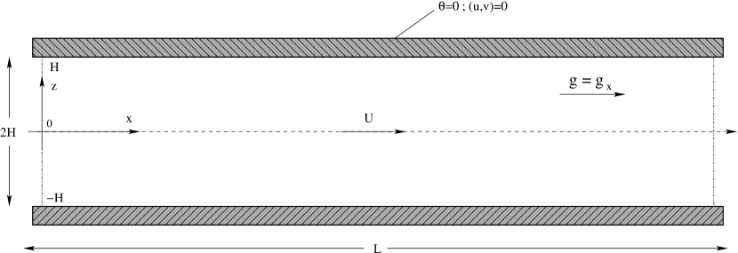
Figure 1: Sketch of the studied system: coordinates and channel dimensions.

In these hypotheses, the fluid dynamics are described by the following transport equations for mass, momentum and energy, respectively:

$$\boldsymbol{\nabla}\boldsymbol{\cdot}{\mathbf{v}}=0$$ (3)

$$\rho\,\frac{\partial{\mathbf{v}}}{\partial t}+\rho{\mathbf{v}}\cdot\boldsymbol{\nabla}{\mathbf{v}}=-\boldsymbol{\nabla}P+\rho{\mathbf{g}}+\boldsymbol{\nabla}\cdot\boldsymbol{\tau}$$ (4)

$$\rho\,\frac{\partial h}{\partial t}+\rho{\bf v}\boldsymbol{\cdot}\boldsymbol{\nabla}h=k{\boldsymbol{\nabla}}^{2}T+\tau_{ij}\frac{\partial v_{i}}{\partial x_{j}}$$ (5)

where $\rho$ is the fluid density, v is the velocity vector, ${\mathbf{g}}$ represents the generic body force, $P$ is the pressure, $\boldsymbol{\tau}$ is the stress tensor, $h$ is the enthalpy per unit mass, $T$ is the temperature, and $k$ is the thermal conductivity. The term containing the stress tensor $\boldsymbol{\tau}$ in equation (5) represents the internal heat generated by the viscous dissipation (Einstein notation of summation over repeated indeces is used). In this study, for simplicity, the latent heat release due to crystallization is not considered, the enthalpy is simply given by the product of a constant specific heat times the temperature. Moreover we neglect any possible effect due to the buoyancy. Under these assumptions and considering a Newtonian relationship between stress tensor and strain-rate ($\tau_{ij}=\mu(\partial v_{i}/\partial x_{j}+\partial v_{j}/\partial x_{i})$), equations (3), (4) and (5) can be easily expressed in dimensionless form as:

$$\frac{\partial u_{i}}{\partial\xi_{i}}=0$$ (6)

$$\frac{\partial u_{i}}{\partial\hat{t}}+u_{j}\frac{\partial u_{i}}{\partial\xi_{j}}=\frac{1}{Fr}\hat{g}_{i}-\frac{\partial p}{\partial\xi_{i}}+\frac{1}{Re}\frac{\partial}{\partial\xi_{j}}\left[e^{-\Theta}\left(\frac{\partial u_{i}}{\partial\xi_{j}}+\frac{\partial u_{j}}{\partial\xi_{i}}\right)\right]$$ (7)

$$\frac{\partial\Theta}{\partial\hat{t}}+u_{j}\frac{\partial\Theta}{\partial\xi_{j}}=\frac{1}{Pe}\frac{\partial}{\partial\xi_{j}}\frac{\partial\Theta}{\partial\xi_{j}}+\frac{Na}{Pe}\frac{e^{-\Theta}}{2}\left(\frac{\partial u_{i}}{\partial\xi_{j}}+\frac{\partial u_{j}}{\partial\xi_{i}}\right)^{2}$$ (8)

where $\hat{t}=tU_{*}/H$ is the dimensionless time, $(\xi_{1},\xi_{2})=(x/H,z/H)$ are the longitudinal and transversal dimensionless coordinates, $(u_{1},u_{2})=(v_{x}/U_{*},v_{z}/U_{*})$ represent the dimensionless field velocities (scaled with the characteristic velocity $U_{*}$), $\Theta=\beta(T-T_{0})$ the dimensionless temperature, $(\hat{g}_{1},\hat{g}_{2})=(g_{x}/|{\mathbf{g}}|,g_{z}/|{\mathbf{g}}|)$ indicate the dimensionless body force field (from here on-wards we set $g_{z}=0$) and $p=P/(\rho U_{*}^{2})$ is the dimensionless pressure (Einstein convention of summation over repeated indeces is used). The meaning of the usual characteristic dimensionless numbers is reported in Table 1.
Due to the symmetry of the channel and of the boundary conditions, we investigate only half of the channel ($0\leq\xi_{2}\leq 1$). At the walls the boundary conditions are given by no-slip velocity and isothermal temperature: $u_{i}=\Theta=0$ at $\xi_{2}=1$ and by $u_{2}=\partial u_{1}/\partial\xi_{2}=\partial\Theta/\partial\xi_{2}=0$ at $\xi_{2}=0$. At the inlet we assume free flow conditions and the fluid temperature to be the same as the wall temperature: $\Theta_{in}=0$. As initial conditions, the velocity and temperature are set equal to zero.

Name	Symbol	Definition	Value	Symbol	Definition	Value
Reynolds number	$Re_{*}$	$\rho U_{*}H/\mu_{0}$	4.5	$Re$	$\rho UH/\overline{\mu}$	119.4
Nahme number	$Na_{*}$	$\beta\mu_{0}U_{*}^{2}/k$	14.4	$Na$	$\beta\overline{\mu}U^{2}/k$	2400
Froude number	$Fr_{*}$	$U_{*}^{2}/(g_{x}H)$	1.5	$Fr$	$U^{2}/(g_{x}H)$	412
Péclet number	$Pe_{*}$	$\rho c_{p}U_{*}H/k$	450	$Pe$	$\rho c_{p}UH/k$	7400
Aspect ratio	$a_{r}$	$H/L$	3/100	$a_{r}$	$H/L$	3/100

Table 1: Typical dimensionless numbers. The calculated values on the left side are based on the mean Poiseuille velocity $U_{P}=\rho g_{x}H^{2}/(3\mu_{0})$. The calculated values on the right side are instead based the mean velocity $U=(\int_{0}^{H}v_{x}dz)/H$ and mean viscosity $\overline{\mu}=(\mu_{0}\int_{0}^{H}\exp(-\Theta))/Hdz$.

Considering the geometry of figure 1 and the isothermal case without viscous heating effects, the Navier-Stokes equations of a viscous liquid driven by a body force $g_{x}$ admit a simple solution (Landau & Lifschitz, 1994):

$$\mu_{0}\displaystyle\frac{d^{2}v_{x}}{dz^{2}}+\rho g_{x}=0\qquad\displaystyle\frac{dP}{dz}=0$$ (9)

In this case, the mean velocity is $U_{P}=\rho g_{x}H^{2}/(3\mu_{0})$.
From this point on-wards, we use starred symbols to indicate the dimensionless number based the characteristic velocity $U_{P}$, i.e. we set $U_{*}=U_{P}$, while the un-starred numbers are based on the mean velocity $U=(\int_{0}^{H}v_{x}dz)/H$, i.e. we set $U_{*}=U$ (see Table 1).
The parameter values used in the DNS and reported in Table 1 are chosen in order to perform the computation in a reasonable time, maintaining the system in the regime with $Re<{\mathcal{O}}(10^{2})$, $Na\gg 1$, $Pe\gg 1$, $Pr\gg 1$ and $H/L\ll 1$. To fully simulate the flow field evolution when viscous heating effects are very important, there is a need to solve all the involved length scales of the problem: from the integral length $H$ up to the smallest characteristic length-scale. The smallest scales correspond to a thin layer of the order of $Gz^{-1/2}(\ln Na)^{-1}$ in which the velocity changes from near zero by the wall to near its core value ($Gz=Pe\times H/L$ indicates the Graetz number) as shown by Pearson (1977) in the asymptotic limit of very large $Na$ and $Gz$.

3 Stability analysis

The stability of a fully developed steady plane Couette flow was recently re-examined by Yueh & Weng (1996), who improved the results previously obtained by Sukanek et al. (1973). The plane Couette flow shows two different instability modes: one arising in the non-viscous limit, and the other due to the viscosity stratification. As far as the last instability mode is concerned, it was demonstrated that the critical Reynolds number, above which the flow becomes turbulent, decreases as the Nahme number increases, that is as the viscous heating increases (Yueh & Weng, 1996).
Viscous heating effects on flow stability have been recently investigated experimentally by White & Muller (2000), who have shown that above a critical Nahme number an instability appears at a Reynolds number one order of magnitude lower than the corresponding Reynolds number predicted for isothermal flow (in these experiments, the authors use a temperature-dependent fluid, i.e. glycerin, and a Taylor-Couette device which allows the tracking of the vortices by a laser particle tracer).

When the viscous heating is relevant ($Na\gg 1$) and the thermal length is much greater than the mechanical one, the temperature profile, which is characterized by a narrow peak near the channel wall, is drastically different from the corresponding profile of a thermally steady fully developed flow (Pearson, 1977; Ockendon, 1979; Costa & Macedonio, 2003). Assuming slow longitudinal variations of velocity and temperature, we now study the linear stability of a thermally developing flow belonging to the important regime with $L_{t}/H=Pe\gg 1$, $L_{t}/L_{m}=Pr\gg 1$, $Gz\gg 1$ that typically characterizes magma flows (Wylie & Lister, 1995). In this regime it is legitimate to use a lubrication approximation.

3.1 Linear stability

For the investigation of the linear stability we use the method of small perturbations (normal-mode analysis). The base velocity, temperature, viscosity and pressure fields are perturbed by two-dimensional, infinitesimal disturbances. Each variable ($u_{i},\Theta,\mu,p$) is given by a steady part plus a small deviation from the steady state:

$$\begin{array}[]{c}u_{1}(\xi_{1},\xi_{2},t)=\overline{u}_{1}(\xi_{2})+\tilde{u}_{1}(\xi_{1},\xi_{2},t)\\ u_{2}(\xi_{1},\xi_{2},t)=\tilde{u}_{2}(\xi_{1},\xi_{2},t)\\ p(\xi_{1},\xi_{2},t)=\overline{p}(\xi_{1})+\tilde{p}(\xi_{1},\xi_{2},t)\\ \Theta(\xi_{1},\xi_{2},t)=\overline{\Theta}(\xi_{1},\xi_{2})+\tilde{\Theta}(\xi_{1},\xi_{2},t)\\ \nu(\xi_{1},\xi_{2},t)=\overline{\nu}(\xi_{1},\xi_{2})+\tilde{\nu}(\xi_{1},\xi_{2},t)\end{array}$$ (10)

where the overbar symbol indicates the steady part, the tilde the perturbation, and $\nu=\mu/\mu_{0}=e^{-\Theta}$ is the dimensionless viscosity. In the (10), the steady part of temperature and viscosity depend on the streamwise coordinate $\xi_{1}$ while the mean flow is assumed not to vary appreciably with $\xi_{1}$ over an instability wavelength. This means that we study the thermally developing flow by making the so called quasi-parallel-flow approximation ($\overline{u_{2}}\simeq 0$). I.e. one examines the stability of a model flow having the same streamwise velocity profile as the real spatially inhomogeneous flow at the selected spatial location. Since we treat the stability of those systems in the limit $Pe\gg 1$ and $Pr\gg 1$, with the characteristic length $L_{t}$ much greater than the other typical mechanical length scales (Pearson, 1977; Ockendon, 1979; Costa & Macedonio, 2003), this assumption is legitimate. In this regime it is also legitimate to assume that the base flow satisfies a system of equations similar to that introduced by Pearson (1977). At a fixed distance from the inlet, we consider the following steady equations:

$$\begin{array}[]{l}\int_{0}^{1}\overline{u}_{1}d\xi_{2}=1\\ \displaystyle\frac{\partial\overline{u}_{1}}{\partial\xi_{2}}=Re\left(\frac{\partial\overline{p}}{\partial\xi_{1}}-\frac{\hat{g}_{1}}{Fr}\right)\xi_{2}e^{\overline{\Theta}}\\ \displaystyle Pe~{}\overline{u}_{1}\frac{\partial\overline{\Theta}}{\partial\xi_{1}}=\frac{\partial^{2}\overline{\Theta}}{\partial\xi_{2}^{2}}+Na\left(\frac{\partial\overline{u}_{1}}{\partial\xi_{2}}\right)^{2}e^{-\overline{\Theta}}\end{array}$$ (11)

with geometry and coordinate system showed in figure 1. As boundary conditions we consider $u_{i}=\Theta=0$ at $\xi_{2}=\pm 1$ whereas at the inlet ($\xi_{1}=0$) we assume a parabolic velocity profile and an uniform temperature ($\overline{\Theta}=0$). Equations (11) were solved by a finite-difference method with an implicit scheme for the integration along direction $\xi_{1}$; the pressure gradient was iteratively adjusted at each step in order to satisfy mass conservation.
In the following, we study the linear stability of the base velocity and temperature profiles given by (11). Since the variations with $\xi_{1}$ depend upon the coupling with the energy equation through the viscosity, we consider slow temperature variations with $\xi_{1}$ (Pearson, 1977). Substituting (10) into the equations (6), (7), (8), subtracting the base flow solutions of (11) and linearizing, we obtain:

$$\frac{\partial\tilde{u}_{1}}{\partial\xi_{1}}+\frac{\partial\tilde{u}_{2}}{\partial\xi_{2}}=0$$ (12)

$$\begin{array}[]{l}\displaystyle\frac{\partial\tilde{u}_{1}}{\partial\hat{t}}+\overline{u}_{1}\frac{\partial\tilde{u}_{1}}{\partial\xi_{1}}+\tilde{u}_{2}\frac{d\overline{u}_{1}}{\partial\xi_{2}}=-\frac{\partial\overline{p}}{\partial\xi_{1}}+\frac{\overline{\nu}}{Re}\left(\frac{\partial^{2}\tilde{u}_{1}}{\partial\xi_{1}^{2}}+\frac{\partial^{2}\tilde{u}_{1}}{\partial\xi_{2}^{2}}\right)+\\ \displaystyle\frac{1}{Re}\frac{d\overline{\nu}}{d\xi_{2}}\left(\frac{\partial\tilde{u}_{1}}{\partial\xi_{2}}+\frac{\partial\tilde{u}_{2}}{\partial\xi_{1}}\right)+\frac{1}{Re}\frac{d\overline{u}_{1}}{d\xi_{2}}\frac{\partial\tilde{\nu}}{\partial\xi_{2}}+\frac{\tilde{\nu}}{Re}\frac{d^{2}\overline{u}_{1}}{d\xi_{2}^{2}}\end{array}$$ (13)

$$\frac{\partial\tilde{u}_{2}}{\partial\hat{t}}+\overline{u}_{1}\frac{\partial\tilde{u}_{2}}{\partial\xi_{1}}=-\frac{\partial\tilde{p}}{\partial\xi_{2}}+\frac{2}{Re}\frac{d\overline{\nu}}{d\xi_{2}}\frac{\partial\tilde{u}_{2}}{\partial\xi_{2}}+\frac{\overline{\nu}}{Re}\left(\frac{\partial^{2}\tilde{u}_{2}}{\partial\xi_{2}^{2}}+\frac{\partial^{2}\tilde{u}_{2}}{\partial\xi_{1}^{2}}\right)+\frac{1}{Re}\frac{d\tilde{\nu}}{d\xi_{1}}\frac{d\overline{u}_{1}}{d\xi_{2}}$$ (14)

$$\begin{array}[]{c}\displaystyle Pe\left(\frac{\partial\tilde{\Theta}}{\partial\hat{t}}+\overline{u}_{1}\frac{\partial\tilde{\Theta}}{\partial\xi_{1}}+\tilde{u}_{1}\frac{\partial\overline{\Theta}}{\partial\xi_{1}}+\tilde{u}_{2}\frac{\partial\overline{\Theta}}{\partial\xi_{2}}\right)=\frac{\partial^{2}\tilde{\Theta}}{\partial\xi_{1}^{2}}+\frac{\partial^{2}\tilde{\Theta}}{\partial\xi_{2}^{2}}+\\ \displaystyle 2\overline{\nu}Na\frac{\partial\overline{u}_{1}}{\partial\xi_{2}}\left(\frac{\partial\tilde{u}_{1}}{\partial\xi_{2}}+\frac{\partial\tilde{u}_{2}}{\partial\xi_{1}}+\frac{\tilde{\nu}}{\overline{\nu}}\frac{\partial\overline{u}_{1}}{\partial\xi_{2}}\right)\end{array}$$ (15)

Equations (12), (13), (14) and (15) are similar to those analyzed by Pinarbasi & Liakopoulos (1995) who investigated how a variable viscosity affects the stability of the system. In this study we account for the longitudinal variation of the base temperature ($\partial\overline{\Theta}/\partial\xi_{1}$) which was not considered by Pinarbasi & Liakopoulos (1995) and we also introduce new terms on the right side of equation (15) related to the viscous heating.
In order to eliminate the continuity equation (12), we introduce a perturbation streamfunction $\tilde{\psi}$:

$$\tilde{u}_{1}=\frac{\partial\tilde{\psi}}{\partial\xi_{2}}\qquad\tilde{u}_{2}=-\frac{\partial\tilde{\psi}}{\partial\xi_{1}}$$ (16)

Moreover we assume that all perturbations have temporal and spatial dependence of the form:

$$(\tilde{\psi},\tilde{p},\tilde{\Theta},\tilde{\nu})=[\phi(\xi_{2}),f(\xi_{2}),\theta(\xi_{2}),\Lambda(\xi_{2})]\ e^{i\alpha(\xi_{1}-c\hat{t})}$$ (17)

where $\alpha$ is the wavenumber, $c$ is the complex perturbation velocity and $\phi,f,\theta,\Lambda$ indicate the disturbance amplitudes.
Substituting equations (16) and (17) into the (12), (13), (14) and (15), and eliminating the pressure disturbance term by cross differentiation and subtraction, we obtain the final stability equations:

$$\begin{array}[]{c}i\alpha Re\left[(\overline{u}-c)(\phi{{}^{\prime\prime}}-\alpha^{2}\phi)-\overline{u}^{{}^{\prime\prime}}\phi\right]=\overline{\nu}(\phi^{iv}-2\alpha^{2}\phi^{{}^{\prime\prime}}+\alpha^{4}\phi)+\\ 2\overline{\nu}^{\prime}(\phi{{}^{\prime\prime\prime}}-\alpha^{2}\phi^{\prime})+\overline{\nu}{{}^{\prime\prime}}(\phi{{}^{\prime\prime}}+\alpha^{2}\phi)+\overline{u}^{\prime}(\Lambda{{}^{\prime\prime}}+\alpha^{2}\Lambda)+2\overline{u}{{}^{\prime\prime}}\Lambda^{\prime}+\overline{u}{{}^{\prime\prime\prime}}\Lambda\end{array}$$ (18)

$$i\alpha Pe\left[(\overline{u}-c)\theta-\phi\overline{\Theta}^{\prime}+\phi^{\prime}\frac{\partial\overline{\Theta}}{\partial\xi_{1}}\right]=(\theta{{}^{\prime\prime}}-\alpha^{2}\theta)+2\overline{\nu}Na\left[(\phi{{}^{\prime\prime}}+\alpha^{2}\phi)+\frac{\Lambda}{\overline{\nu}}\overline{u}^{\prime}\right]\overline{u}^{\prime}$$ (19)

where for simplicity with $\overline{u}$ we indicate the velocity base flow $\overline{u}_{1}$ and the symbol prime indicates differentiation with respect to $\xi_{2}$. Viscosity perturbation $\Lambda$ can be expressed in terms of temperature fluctuations by the Taylor expansion of (2), and neglecting nonlinear terms:

$$\Lambda=-\theta\bar{\nu}$$ (20)

obtaining the two final governing stability equations for $\phi$ and $\theta$. Finally, as boundary conditions for (18) and (19), we consider:

$$\phi=0,\quad\phi^{\prime}=0,\quad\theta=0\qquad\mbox{at}\quad\xi_{2}=\pm 1$$ (21)

We note that equation (18) reduces to the classical Orr-Sommerfeld equation when $\bar{\nu}=1$ and the equation (19) reduces to that used by Pinarbasi & Liakopoulos (1995) when both $Na=0$ and $\partial\overline{\Theta}/\partial\xi_{1}=0$.

3.2 Solution method and stability results

Classical flow stability problems are usually approached in two ways: temporal and spatial. In the former case, it is assumed that small disturbances evolve in time from some initial spatial distribution. In this case, for an arbitrary positive real value of $\alpha$, the complex eigenvalue $c=c_{R}+ic_{I}$ and the corresponding eigenfunctions $\phi$ and $\theta$ are obtained. If $c_{I}=\mbox{Im}(c)$ is negative then the flow is temporally stable, otherwise it is unstable.
The spatial analysis is focused on the spatial evolution of a time periodic perturbation at a fixed position in the flow. This study requires the solution of a nonlinear eigenvalue problem in $\alpha$, which is assumed complex $\alpha=\alpha_{R}+i\alpha_{I}$ with a prescribed real $c=c_{R}$. The disturbances grow for $\mbox{Im}(\alpha)<0$ and decay for $\mbox{Im}(\alpha)>0$.
The choice between spatial and temporal study depends on the nature of the flow instability considered (see Huerre & Monkewitz, 1990, for a general review ). Moreover quasi-parallel flows may contain different region with different stability characteristics.
In the present paper, a temporal stability analysis of the profiles at a selected set of distances from the inlet, has been performed. This analysis is adequate for studying the so-called absolute instabilities (i.e. when the perturbation contaminates the entire flow both upstream and downstream of the source location).

3.2.1 Temporal stability study

The problem formulated in the § 3.1 is solved using a Chebyshev collocation technique, expanding the functions $\phi$ and $\theta$ in series of Chebyshev polynomials of order N. The 2(N+1) coefficients are considered as unknowns and they are evaluated by the collocation technique applied at points $\xi_{2,i}=\cos(\frac{\pi i}{N-3})$ with $i=0,1,2,3...N-3$ and imposing the six boundary conditions (21) at $\xi_{2}=\pm 1$. This method allows us to define a system of $2(N+1)$ equations in $2(N+1)$ unknowns which can be written as a generalized eigenvalue problem of the type Ax=cBx. The final system was solved using the LAPACK routine ZGGEV. Typically, setting $N=70$ and $N=80$ permits a satisfactory convergence in the computation of the eigenvalues. In order to test the above described computational implementation we compared the obtained eigenvalues in the limit $\Theta\rightarrow 0$, with Orszag (1971)’s results (considering Orszag’s definitions, our $c$ is 1.5 times Orszag’s $c$ while Orszag’s $Re$ is 1.5 times our $Re$). Table 2 shows that eigenvalues we calculated for isothermal limits are very close to those obtained by Orszag (1971).

Mode Number	Eigenvalues by Orszag (1971)	Our eigenvalues for $\Theta=0$
1	0.23752649 + 0.00373967 i	0.237526311 + 0.00373795 i
2	0.96463092 - 0.03516728 i	0.964629174 - 0.03516535 i
3	0.96464251 - 0.03518658 i	0.964643595 - 0.03518749 i
4	0.27720434 - 0.05089873 i	0.277207006 - 0.05089868 i
5	0.93631654 - 0.06320150 i	0.936328259 - 0.06320707 i
…	…	…

Table 2: Least stable eigenvalues $c=c_{R}+ic_{I}$ calculated in this work in the isothermal limit compared with the Orszag (1971)’s results for $Re=10^{4}$ and $\alpha=1$. $N=70$ was set.

As far as the base flow is concerned, we considered a fixed distance from the inlet $\xi_{1}^{*}$ and a given Péclet number $Pe$. As shown in figure 2 for $Pe=10^{7}$, as the Nahme number increases, velocity distributions deviate from parabolic profile and dimensionless viscosity drops near the walls.

Figure 2: Base velocity profiles (on the left) and base viscosity profiles (on the right) at $\xi_{1}^{*}=100$ for $Pe=10^{7}$ and for $Na=0;1;10;100;1000$. Here velocity profiles are normalized with respect to the mean velocity $U$.

The stability analysis shows that viscous heating in fluids with temperature-dependent viscosity is destabilizing. In fact in the cases studied, for a given $Pr$ there is a critical Nahme number $Na_{c}$ above which the flow is unstable at any $Re$, i.e. the critical Reynolds number $Re_{c}$ decreases as the Nahme number $Na$ increases. Two clear examples of this are shown in figure 3 where, for different values of $Na$, the imaginary part of the eigenvalue $c$ is plotted as a function of the wavenumber $\alpha$ at a distance $\xi_{1}^{*}=100$ from the inlet and for $(Re=10^{2},Pr=10^{5})$ and $(Re=10^{3},Pr=10^{4})$, respectively. From these plots, it is evident that increasing the Nahme number, the imaginary part of the complex perturbation velocity tends to increase until becomes positive. For instance, for $Pr=10^{5}$ and $Re=10^{2}$ the flow becomes unstable for $Na\lesssim 10^{3}$ while at $Pr=10^{5}$ and $Re=10^{3}$ the flow is unstable for $Na\gtrsim 10$. The same behaviour was observed with lower Reynolds number where the flow becomes unstable at larger $Na$.

Figure 3: Imaginary part of the complex perturbation velocity vs $\alpha$: $Pr=10^{4}$, $Re=10^{3}$ (on the left) and $Pr=10^{5}$ and $Re=10^{2}$ (on the right). For both cases a distance from the inlet of $\xi_{1}^{*}=100$ was set.

Beside the investigation of the role of the Nahme and Reynolds numbers on the flow stability, a more deepened parametric study of the effects of the other controlling parameters of the problem, such as the Péclet number and the distance from the inlet, should be performed. In any case, even considering our preliminary results, it is clear that viscous heating effects in fluids with temperature-dependent viscosity are important for the determination of flow instablities and, without their inclusion, the critical Reynolds number is generally overestimated.

4 Numerical simulation

In this section, we first describe the numerical scheme, then the numerical parameters used to solve the equations described above and, finally, we present the results obtained and discuss them.

4.1 Numerical scheme

To solve equations (3), (4) and (5), a fortran code based on the Finite Element Method (FEM) with the Streamline-Upwind/Petrov-Galerkin (SU/PG) scheme (Brooks & Hughes, 1982) was used. The enthalpy equation is added in a similar way as suggested by Heinrich & Yu (1988). The solution method is explicit in the velocity and temperature and implicit in the pressure, which is computed solving a Poisson equation.
The domain of interest $\Omega$ is partitioned into a number of non intersecting elements $\Omega^{e}$ with $e$=1,2,…,$n_{e}$, where $n_{e}$ is the total number of elements. In contrast with the usual Galerkin method, which considers the weighting functions continuous across the element boundaries, the SU/PG formulation requires discontinuous weighting functions of the form: $\tilde{w}=w+\tilde{s}$, where $w$ is a continuous weighting function (the Galerkin part) and $\tilde{s}$ is the discontinuous streamline upwind part. Both $w$ and $\tilde{s}$ are smooth inside the element. The upwinding functions $\tilde{s}$ depend on the local element Reynolds number (momentum equations) and the local element Péclet number (enthalpy equation). The SU/PG weighting residual formulation of the initial-boundary value problem defined by equations (3) and (4) can be respectively recasted as:

$$\sum_{e}\int_{\Omega_{e}}\tilde{s}^{p}_{k}\,\frac{\partial v_{i}}{\partial x_{i}}\,d\Omega=0$$ (22)

where $\tilde{s}^{p}_{k}$ is a weighting function which is chosen to be constant within each element, and discontinuous across the element boundaries, and

$$\begin{array}[]{l}\displaystyle\hbox to0.0pt{$\displaystyle\int_{\Omega}w_{k}\left(\rho\,\frac{\partial v_{i}}{\partial t}+\rho v_{j}\,\frac{\partial v_{i}}{\partial x_{j}}-\rho g_{i}\right)d\Omega+\int_{\Omega}\sigma_{ij}\,\frac{\partial w_{k}}{\partial x_{j}}\,d\Omega\,+$\hss}\\ \displaystyle+\sum_{e}\int_{\Omega}\tilde{s}_{k}^{u}\left(\rho\,\frac{\partial v_{i}}{\partial t}+\rho v_{j}\,\frac{\partial v_{i}}{\partial x_{j}}-\frac{\partial\sigma_{ij}}{\partial x_{j}}-\rho g_{i}\right)d\Omega=\int_{\Gamma_{\sigma}}\sigma_{0i}\,w_{k}\,d\Gamma\end{array}$$ (23)

where $\tilde{s}_{k}^{u}$ is the upwinding function for the momentum equation, $\sigma_{ij}=-P\delta_{ij}+\tau_{ij}$ ($\delta_{ij}$ is the Kronecker symbol). With $\Gamma_{\phi}$ we generally indicate the boundary surface where the variable $\phi$ is prescribed.
In the same way, the weak form of the enthalpy equation (5) may be written as:

$$\begin{array}[]{l}\displaystyle\hbox to0.0pt{$\displaystyle\int_{\Omega}w_{k}\left(\rho\,\frac{\partial h}{\partial t}+\rho v_{i}\,\frac{\partial h}{\partial x_{i}}\right)d\Omega+\int_{\Omega}\left(k\,\frac{\partial T}{\partial x_{i}}\right)\frac{\partial w_{k}}{\partial x_{i}}\,d\Omega\,+$\hss}\\ \displaystyle+\sum_{e}\int_{\Omega}\tilde{s}_{k}^{h}\left[\rho\,\frac{\partial h}{\partial t}+\rho v_{i}\,\frac{\partial h}{\partial x_{i}}-\frac{\partial}{\partial x_{i}}\!\left(k\,\frac{\partial T}{\partial x_{i}}\right)+\tau_{ij}\,\frac{\partial v_{i}}{\partial x_{j}}\right]d\Omega=\int_{\Gamma_{h}}q_{0}\,d\Gamma\end{array}$$ (24)

where, $\tilde{s}_{k}^{h}$ is the upwinding function of the enthalpy equation and $q_{0}$ is the heat flux through the boundary surface $\Gamma_{h}$. In the present work, the velocity field $v$ and the enthalpy fields are linearly interpolated with multi-linear iso-parametric interpolation functions using rectangular elements. The pressure field $P$, instead, is assumed to be constant within each element and discontinuous across the element boundaries.
Equations (23) and (24) yield two algebraic equations which may be combined in the following one:

$$\mathbf{Ma+Cv+N(v)-GP=F}$$ (25)

whilst the continuity equation (22) yields to:

$$\mathbf{G^{T}v=D}$$ (26)

In the above equations, the vector $\mathbf{v}$ represents the nodal values of the velocity $v_{i}$ and the temperature $T$, whereas the vector $\mathbf{a}$ represents the nodal values of the time derivatives of the velocity $\dot{v}_{i}$ and of the temperature $\dot{T}$, $\mathbf{P}$ indicates the pressure field, ${\bf M}$ is the consistent generalised mass matrix, ${\bf C}$ and ${\bf N(v)}$ account for the diffusive and the nonlinear convective terms respectively, ${\bf F}$ is a generalised force vector, ${\bf D}$ accounts for the prescribed velocity at the boundaries, ${\mathbf{G}}$ is the gradient operator, and ${\mathbf{G^{T}}}$ its transpose. Equations (25) and (26) are integrated in time starting from the velocity and pressure fields at $t=0$.
Convergence of the algorithm is assured when the element Courant number $Cr$ satisfies particular conditions depending on the element Reynolds and Péclet numbers. Typically, to assure the convergence, the element Courant number should satisfy the most restrictive among the following relations (Brooks & Hughes, 1982):

$$Cr\leq 0.8,\qquad \quad\gamma=\left\{{}^{\displaystyle Re_{el}}_{\displaystyle Pe_{el}}\geq 100,\right.$$ if

$$Cr\leq\hbox{min}(1,\gamma),\qquad \quad\gamma=\left\{{}^{\displaystyle Re_{el}}_{\displaystyle Pe_{el}}<100\right.$$ if

where $Cr=v\Delta t/\Delta x_{i}$, with $v$, $\Delta t$ and $\Delta x_{i}$ element velocity, computational time step and computational grid size respectively, and $\gamma=Re_{el}\mbox{ or }Pe_{el}$ represents both the element Reynolds and Péclet numbers. Unfortunately, the above convergence criteria can be very restrictive, forcing the choice of a very small time step to guarantee the convergence of the algorithm.

4.2 Numerical parameters

Since viscous friction is greater near the walls (higher gradients), it is convenient to use a computational grid finer near the boundaries and coarser towards the centre of the channel.
The computational grid was formed by an uniform horizontal grid size $\Delta x/H=8.3\cdot 10^{-2}$ while the vertical mesh size $\Delta\zeta=\Delta z/H$ is not uniform and consists of three different grid sizes $\Delta\zeta_{1}$, $\Delta\zeta_{2}$, and $\Delta\zeta_{3}$. The finest grid size $\Delta\zeta_{1}=1.67\cdot 10^{-2}$ was set near the wall where the fields change rapidly and the viscosity is lower, $\Delta\zeta_{2}=3\cdot 10^{-2}$ was set in the intermediate region and finally, $\Delta\zeta_{3}=4.67\cdot 10^{-2}$ in the central part of the channel. The computational grid used for the simulations is shown in figure 4.
A time step of $\Delta\hat{t}=5\cdot 10^{-4}$ was chosen to perform the simulation, with one predictor and one corrector iterations per time step, whereas spatial integration was performed using a 2x2 Gauss quadrature. All runs were performed in double-precision arithmetics on a HP-J5600 workstation.
From a practical point of view, an estimation of the minimum grid size required to well resolve the rapidly varying fields was assumed to be equal to the smallest scale involved in the problem (Pearson, 1977): $\Delta\zeta_{1}^{(0)}=Gz^{-1/2}(\ln Na)^{-1}$ (using some $Na$ and $Gz$ initial estimations), it was then further reduced to guarantee the numerical convergence and in such a way that the numerical solution does not appreciably depend on the computational grid size. The final dimensionless numbers used in the DNS are reported in Table 1.

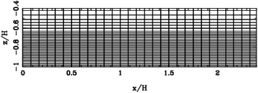
Figure 4: Zoom of the bottom-left corner of the computational grid used for the simulations. The entire computational domain was discretized with $401\times 38$ rectangular elements. The longitudinal grid size was chosen uniform $\Delta x/H=8.3\cdot 10^{-2}$ while three different sizes were used to form the transverse grid: $n_{1}=23$ elements of size $\Delta z_{1}/H=1.67\cdot 10^{-2}$ near the wall, $n_{2}=5$ elements of size $\Delta z_{2}/H=3\cdot 10^{-2}$ in the intermediate region, and $n_{3}=10$ elements of size $\Delta z_{2}/H=4.67\cdot 10^{-2}$ in the central part of the channel.

4.3 Results and discussion

In this section we describe results obtained by the direct numerical simulation (using the FEM code described in § 4.1) for the values of the parameters reported in § 4.2 and Table 1 for a channel flow of length 100/3 $H$-unit.

In this study we relied on the small numerical round-off errors present in any numerical simulation to trigger natural modes, but further cases with e.g. selected harmonic or random input disturbance should be investigated.

From these simulations we can see that as the time increases the temperature starts to rise in the region near the outlet because of viscous heating. At $\hat{t}=\hat{t}_{c}\approx 40$ an instability is triggered in this region where the dimensionless temperature $\Theta$ locally becomes greater than $\approx 5$ (see figure 5). For $\hat{t}>\hat{t}_{c}$, as viscous heating effects become more important even in the more internal region, secondary flows appear to organize themselves into “coherent structures” as rotational flows. This kind of secondary flow looks like roller vortices which seem to move from the region near the outlet towards the inlet (see figure 5). Actually this happens because the viscous heating becomes relevant even in the internal region and the entire flow becomes unstable.
Figure 7 show the temporal profile evolution at a given distance (for example at $\xi_{1}=22$ that is about 2/3 of the channel length). We can see that $\Theta$, starting with a flat distribution, gradually increases near the wall forming a profile with a maximum at a short distance from the boundary. As time increases, this peak becomes more pronounced ($\Theta_{max}\lesssim 6$) filling, at the steady state, a narrow shell of values at a shorter distance from the wall (see figure 7). As a consequence the dimensionless viscosity profile $e^{-\Theta}$, strongly decreases in correspondence of the temperature peak, reaching values much samller than its initial ones (see figure 7). The layer where the viscosity is very small is immediately close to the colder layer adjacent to the wall and it corresponds to the region where the vortices appear (see figures 5).
The longitudinal velocity profile (scaled by $U_{P}$), starting with a parabolic distribution, evolves toward a plug profile filling, at the steady state, a narrow region of values with a plug velocity $\lesssim 18$ (see figure 8). Figure 8 also shows the evolution of the transversal dimensionless velocity profiles which, because of the vortical motions, near the wall, tend to fill an onion shape region with the largest fluctuations in corrispondence of the peak in the temperature profile. For comparison, the profiles computed using the lubrication approximation (11) are reported in figures 7 and 8.

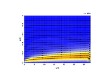
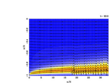
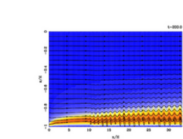
Figure 5: Evolution of the dimensionless flow fields. The figures show the simulated streamlines with the temperature field as background at different times $\hat{t}$. The values reported along vertical and horizontal axes indicate the dimensionless distances from the channel wall and from the inlet, respectively. The blue colour indicates the lowest dimensionless temperature ($\Theta=0$) and the dark orange corresponds to the highest temperature ($\Theta=6$). The symbol $t$ on the upper right corner indicates the dimensionless time $\hat{t}$. For visualization reasons the horizontal axis is contracted with respect to the vertical.

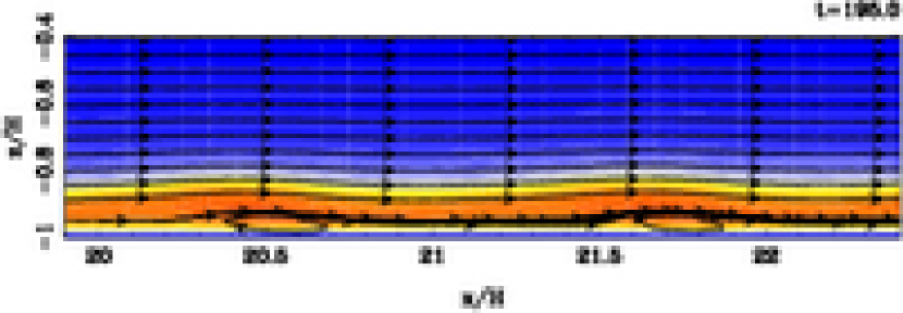
Figure 6: Visualization of the flow structures near the channel wall for $\hat{t}=195$ at a dimensionless distance from inlet of about 2/3 of the channel length. The blue colour indicates the lowest dimensionless temperature ($\Theta=0$) and the darkest orange corresponds to the highest temperature ($\Theta=6$).

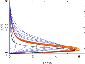
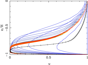
Figure 7: Temporal evolution from $\hat{t}=0$ (blue colour) to $\hat{t}=250$ (red colour) of dimensionless temperature profile $\Theta$ (on the left) and dimensionless viscosity profile $\nu$ (on the right), at a dimensionless distance from inlet of about 2/3 of the tube length ($\xi_{1}^{*}=22$). The coding colour maps the time evolution from the blue up to red. For comparison, temperature and viscosity profiles computed using the lubrication approximation (equations (11)) are also reported (full lines with crosses).

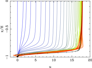
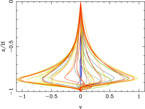
Figure 8: Temporal evolution from $\hat{t}=0$ (blue colour) to $\hat{t}=250$ (red colour) of the profile of the dimensionless longitudinal velocity $u=u_{1}=v_{x}/U_{P}$ (on the left) and of the dimensionless transversal velocity profile $v=u_{2}=v_{z}/U_{P}$ (on the right), at a dimensionless distance from inlet of about 2/3 of the tube lenght ($\xi_{1}^{*}=22$). The coding colour maps the time evolution from the blue up to red. For comparison, the velocity profile computed using the lubrication approximation (equations (11)) is also reported (full line with crosses).

Some of these results could be expected on physical basis. In fact, as a first approximation, because of viscous dissipation effects, the flow can be viewed as a two-layer-flow of two different viscosity fluids with the less viscous one flowing near the wall. The simulations perfomed confirm this limit, in fact when viscous heating form a consistent layer of less viscous liquid near the wall, the behaviour of this flow tends to be similar to that of a two-layer flow with the more viscous fluid in the central part and the less viscous fluid near the wall. This arrangement is common in transporting heavy viscous oils which are lubricated using a sheath of lubricating water (Joseph et al., 1997; Li & Renardy, 1999). Experiments and simulations of this two-layer flow type of fluids with high viscosity ratio predict spatially periodic waves called bamboo waves because of their shape, and the formation of vortices in the region near the wall distributed in the trough of the waves (Joseph et al., 1997).
In our simulations, these features can be seen from figure 5 and from figure 6 where a zoom of the flow fields near the channel wall is shown. In fact following the flow isolines, a spatially periodic wave can be easily discerned and relatively large vortices, settled in the middle of the wave troughs, are also evident.
Moreover, similarly to the core-annular flows with high viscosity ratio (Li & Renardy, 1999), the formation of a mixed profile (with a counter-flow zone) near the wall, leads to the appearance of vortices (figure 8).
Finally, using the dimensionless numbers reported in Table 1, we perfomed a linear stability analysis of the base profiles given by the lubrication approximation (11) at a distance 2/3 of the tube length ($\xi_{1}^{*}\simeq 22$) from the inlet. These analysis indicate that the base flow is already unstable for $Na\lesssim 120$ even at $Re=120$ and, as it is shown in figure 9, the most dangerous mode for this flow has wave number $\alpha\approx 7$, corresponding to a wave length $\lambda\simeq 1.1$ (in $H$-unit) which appears in agreement with that given by DNS. In fact, as it is shown in figure 6, at the distance $\xi_{1}^{*}\approx 22$ from the inlet, a wave length of $\lambda\approx 1.2$ can be estimated.
In order to obtain a closer comparison of the linear stability theory with the nonlinear results obtained by the numerical code above presented, we simulated the case of a channel flow like that previously described, with conditions at the inlet given by the solutions of the equations (11) for $Pe=7400$, $Re=119.4$ and $Na=200$ at $\xi_{1}=21$, free flow conditions in the remaining boundary and no-slip conditions at the walls; as initial field inside the tube we imposed $u_{i}=\theta=0$. The linear theory predicted for these profiles a growth rate $\sigma=\alpha c_{i}\simeq 0.42$ (in $U/H$-unit). To compare the linear with the nonlinear regimes, the evolution of the maximum amplitude $A(t)$ with time (in $H/U$-unit) is plotted in figure 10. The maximum amplitude growth shown in figure 10 is given by the evolution of streamlines around a short distance from the inlet ($0\leq\xi_{1}\leq 1.3$). As initial amplitude we considered the value of $A(t)$ at the time at which small perturbations due to round-off errors begin to grow. Figure 10 shows that the initial evolution of the perturbation is close to that predicted by the linear theory, and then rapidly starts to deviate as amplitude increases. After only less than about one time $H/U$ the linear growth completely fails in the prediction of the amplitude evolution.

These and other preliminary results of the investigations on viscous heating effects (e.g.  Costa & Macedonio, 2003) may help in the understanding of some common phenomena that may occur during lava and magma flows. For instance, effects of viscous dissipation can efficiently enhance thermal and mechanical wall erosion, and can help to understand the reasons of the inadequacy of simple conductive cooling models commonly used to describe lava and magma flows. Moreover in volcanic conduits viscous heating could play an important role on the dynamics of both effusive and explosive eruptions, influencing directly or indirectly magma gas exsolution and fragmentation (Vedeneeva et al., 2005). Since magma flowing in conduits and channels is much hotter than the wall rock, another dimensionless number ${\mathcal{B}}=\beta(T_{in}-T_{w})$, that compares the imposed difference of temperature with $\beta$ should be considered ($T_{in}$ and $T_{w}$ represent inlet and wall temperatures respectively). However, previous preliminary studies indicate that in magma flows, viscous dissipation effects can overcomes the thermal cooling from the walls (Costa & Macedonio, 2003). Moreover, although by increasing ${\mathcal{B}}$ the peak in the temperature profile moves towards the centre of the channel, because of the low magma thermal conductivities, the flow behaviour is not much different from the case with ${\mathcal{B}}=0$ (Costa & Macedonio, 2003; Schneider, 1976).

Figure 9: Imaginary part of the complex perturbation velocity vs $\alpha$: $Pe=7400$, $Re=119.35$ and $Pr=62$ at a dimensionless distance from inlet of about 2/3 of the channel length ($\xi_{1}^{*}=21$).

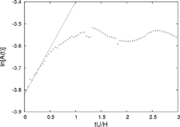
Figure 10: Maximum amplitude $A(t)$ versus time (in $H/U$-unit) on a $\ln$-linear scale. Solid line represents theoretical linear growth and crosses represent simulation.

4.4 Validity and limits of the model

We have seen that when viscous heating is relevant, a special class of secondary flows can develop in fluids with temperature dependent viscosities even at low Reynolds numbers. This kind of vortical structures is locally confined near the walls where there is a large viscosity gradient and the viscosity is lower.

The results obtained are valid in the limit of a 2D model based on the full solution of the Navier-Stokes equations although turbulence is generally three-dimensional even starting with two-dimensional initial conditions. On the other hand, it is known that the growth of three-dimensional instabilities may be suppressed by a strong anisotropy (Sommeria & Moreau, 1982; Messadek & Moreau, 2001). This anisotropy can be due to the presence of a magnetic field (Sommeria & Moreau, 1982), a strong rotation and/or a density stratification (Lilly, 1972; Hopfinger, 1987; van Heijst, 1993).
As in the isothermal case, the Squire’s theorem suggests that for the linear stability analysis it is sufficient to consider two dimensional disturbances. Although the case of core-annular flows with high viscosity ratio suggests that a 2D model is able to describe well the flow features observed during the experiments (Joseph et al., 1997; Li & Renardy, 1999), because of the complexity of these non-isothermal flows, the effects of 3D disturbances on a quasi-2D flow should be also investigated in order to understand whether the evolution of three dimensional motions could be able to obscure the vortical structures described above. In our case, we suppose that the strong viscosity stratification induced by viscous heating could inhibit 3D motions and the 2D model we used should be able to account for the essential physical properties of the real systems; however only an extended 3D simulation can completely confirm this.
Finally, we note that the numerical scheme we used has a first-order upwind and it needs very restrictive conditions and a large computational time in order to be accurate. A more efficient scheme should be used to permit a more complete parametric study.

Conclusions

The thermo-fluid-dynamics of a fluid with strongly temperature-dependent viscosity in a regime with low Reynolds numbers, high Péclet and high Nahme numbers were investigated by direct numerical simulation (DNS) and the linear stability equations of the steady thermally developing base flow was studied.
Our results show that viscous heating can drastically change the flow features and fluid properties. The temperature rise due to the viscous heating and the strong coupling between viscosity and temperature can trigger an instability in the velocity field, which cannot be predicted by simple isothermal Newtonian models.
Assuming steady thermally developing flow profiles we performed a linear stabilty analysis showing the important destabilizing effects of viscous heating.
By using DNS, we showed as viscous heating can be responsible for triggering and sustaining a particular class of secondary rotational flows which appear organized in coherent structures similar to roller vortices.
We wish our preliminary results can stimulate further more accurate studies on this intriguing topic, contributing to a more quantitative comprehension of this problem which has many practical implications such as in the thermo-dynamics of magma flows in conduits and lava flows in channels.