Instability Versus Equilibrium Propagation of Laser Beam in Plasma

Abstract

We obtain, for the first time, an analytic theory of the forward stimulated Brillouin scattering instability of a spatially and temporally incoherent laser beam, that controls the transition between statistical equilibrium and non-equilibrium (unstable) self-focusing regimes of beam propagation. The stability boundary may be used as a comprehensive guide for inertial confinement fusion designs. Well into the stable regime, an analytic expression for the angular diffusion coefficient is obtained, which provides an essential correction to a geometric optic approximation for beam propagation.

Laser-plasma interaction has both fundamental interest and is critical for future experiments on inertial confinement fusion (ICF) at the National Ignition Facility (NIF)Lindl1995 . NIF’s plasma environment, in the indirect drive approach to ICF, has hydrodynamic length and time scales of roughly millimeters and 10 ns respectively, while the laser beams that traverse the plasma, have a transverse correlation length, $l_{c}$, of a few microns, and coherence time $T_{c}$ of roughly a few ps. These microscopic fluctuations induce corresponding small-scale density fluctuations and one might naively expect that their effect on beam propagation to be diffusive provided self-focusing is suppressed by small enough RoseDuBois1993 $T_{c}$, $T_{c}\ll l_{c}/c_{s}$, with $c_{s}$ the speed of sound. However, we find that there is a collective regime of the forward stimulated Brillouin scattering SchmittAfeyan1998 (FSBS) instability which couples the beam to transversely propagating low frequency ion acoustic waves. The instability has a finite intensity threshold even for very small $T_{c}$ and can cause strong non-equilibrium beam propagation (self-focusing) as a result.

We present for the first time, an analytic theory of the FSBS threshold in the small $T_{c}$ regime. In the stable regime, an analytic expression for the beam angular diffusion coefficient, $D$, is obtained to lowest order in $T_{c}$, which is compared with simulation. $D$ may be used to account for the effect of otherwise unresolved density fluctuations on beam propagation in a geometric optic approximation. This would then be an alternative to a wave propagation code StillBergerEtAl2000 , that must resolve the beam’s correlation lengths and time, and therefore is not a practical tool for exploring the large parameter space of ICF designs. Knowledge of this FSBS threshold may be used as a comprehensive guide for ICF designs. The important fundamental conclusion is, for this FSBS instability regime, that even very small $T_{c}$ may not prevent significant self-focusing. It places a previously unknown limit in the large parameter space of ICF designs.

We assume that the beam’s spatial and temporal coherence are linked as in the induced spatial incoherence LehmbergObenschain1983 method, which gives a stochastic boundary condition at $z=0$ ($z$ is the beam propagation direction ) for the various Fourier transform components comment2 , $\hat{E}$, of the electric field spatial-temporal envelope, $E$,

$$\hat{E}({\bf k},z=0,t)=|\hat{E}({\bf k})|\exp\Big{[}i\phi_{\bf k}(t)\Big{]},$$

$$\Big{\langle}\exp i\Big{[}\phi_{\bf k}(t)-\phi_{{\bf k}^{\prime}}(t^{\prime})\Big{]}\Big{\rangle}=\delta_{{\bf kk}^{\prime}}\exp\Big{(}-|t-t^{\prime}|/T_{c}\Big{)}.$$ (1)

The amplitudes, $|\hat{E}({\bf k})|$, are chosen to mimic that of actual experiments, as in the idealized ”top hat” model of NIF optics:

$$|\hat{E}({\bf k})|=const,\ k<k_{m};\ |\hat{E}({\bf k})|=0,\ k>k_{m},$$ (2)

with $1/l_{c}\equiv k_{m}\simeq k_{0}/(2F)$, $F$ the optic $f/\#$, and the average intensity, $\Big{\langle}I\Big{\rangle}\equiv\Big{\langle}|E|^{2}\Big{\rangle}=I_{0}$ determines the constant. At electron densities, $n_{e}$, small compared to critical, $n_{c}$, and for $F^{2}\gg 1$, $E$ satisfies comment3

$$\Big{(}i\frac{\partial}{\partial z}+\frac{1}{2k_{0}}\nabla^{2}-\frac{k_{0}}{2}\frac{n_{e}}{n_{c}}\rho\Big{)}E=0,\ \nabla=(\frac{\partial}{\partial x},\frac{\partial}{\partial y}).$$ (3)

$k_{0}$ is $\simeq$ the laser wavenumber in vacuum. The relative density fluctuation, $\rho=\delta n_{e}/n_{e}$, absent plasma flow and thermal fluctuations which are ignored here, propagates acoustically with speed $c_{s}$:

$$(R_{0}^{\rho\rho})^{-1}\ln(1+\rho)\equiv\Big{(}\frac{\partial^{2}}{\partial t^{2}}+2\tilde{\nu}\frac{\partial}{\partial t}-c_{s}^{2}\nabla^{2}\Big{)}\ln(1+\rho)=c_{s}^{2}\nabla^{2}I.$$ (4)

$\tilde{\nu}$ is an integral operator whose Fourier transform is $\nu kc_{s}$, where $\nu$ is the Landau damping coefficient. $E$ is in thermal units defined so that in equilibrium the standard $\rho=\exp(-I_{0})-1$ is recovered. The physical validity of Eqs. $(\ref{Eeq1}),(\ref{neq1})$ as a model of self-focusing in plasma has been discussed before KawSchmidtWilcox1973 ; SchmittOng1983 ; Schmitt1988 . If $n_{e}/n_{c}$ is taken constant, there are 3 dimensionless parameters for $\rho\ll 1$: $\nu$,$\,\tilde{I}_{0}\equiv(k_{0}/k_{m})^{2}(n_{e}/n_{c})I_{0}/\nu,\,$ and $\tilde{T}_{c}\equiv k_{m}c_{s}T_{c}$.

Since Eqn. $(\ref{Eeq1})$ is linear in $E$, it may be decomposed, at any $z$, into a finite sum, $E=\sum_{j}E_{{\bf m}_{j}}({\bf x},z,t)$, where each term has a typical wavevector ${\bf m}_{j}:$ $E_{{\bf m}_{j}}({\bf x},z=0,t)\sim\exp(i{{\bf m}_{j}}\cdot{\bf x})$. Cross terms $E_{{\bf m}_{j}}E^{*}_{{\bf m}_{j^{\prime}}},\ {\bf m}_{j}\neq{{\bf m}_{j}^{\prime}}$, in the intensity, vary on the times cale $\tilde{T}_{c}$ so that their effect on the density response, Eq. $(\ref{neq1})$, is suppressed for $\tilde{T}_{c}\ll 1$ (see detailed discussion in RoseDuBoisRussell1990 ). Similar consideration may be applied to general media with slow nonlinear response, including photorefractive media Segev1997 . Then the rhs of Eq. $(\ref{neq1})$ can be approximated as

$$c_{s}^{2}\nabla^{2}I=c_{s}^{2}\nabla^{2}\sum\limits_{j}|E_{{\bf m}_{j}}|^{2}=c_{s}^{2}\nabla^{2}\int d{\bf v}F({\bf x},{\bf v},z,t).$$ (5)

$$F({\bf x},{\bf v},z,t)=\int d{\bf r}\sum\limits_{jj^{\prime}}\delta_{{\bf m}_{j}{\bf m}_{j^{\prime}}}$$

$$\times E_{{\bf m}_{j}}({\bf x}-{\bf r}/2,z,t)E^{*}_{{\bf m}_{j^{\prime}}}({\bf x}+{\bf r}/2,z,t)e^{i{\bf v}\cdot{\bf r}}/(2\pi)^{2}$$ (6)

is a variant of the Wigner distribution function which satisfies, as follows from Eq. $(\ref{Eeq1})$,

$$\frac{\partial F}{\partial z}+2{\bf v}\cdot\frac{\partial F}{\partial{\bf x}}-\frac{i}{\pi^{2}}\int\Big{[}\hat{\rho}\big{(}-2[{\bf v}-{\bf v}^{\prime}],z,t\big{)}\times$$

$$\exp\big{(}-2i[{\bf v}-{\bf v}^{\prime}]\cdot{\bf x}\big{)}-\hat{\rho}\big{(}2[{\bf v}-{\bf v}^{\prime}],z,t\big{)}\times$$

$$\exp\big{(}2i[{\bf v}-{\bf v}^{\prime}]\cdot{\bf x}\big{)}\Big{]}F({\bf x},{\bf v}^{\prime},z,t)d{\bf v}^{\prime}=0,$$ (7)

with boundary value $F({\bf x},{\bf v},z=0,t)\equiv F_{0}({\bf v})=|\hat{E}({\bf v})|^{2}$. Here the unit of $x$ is $(1/k_{0})\sqrt{n_{c}/n_{e}}$ and that of $z$ is $(2/k_{0})n_{c}/n_{e}$. Zero density fluctuation, $\rho=\partial\rho/\partial t=0,$ is an equilibrium solution of (4), $(\ref{nFeq1})$ and $(\ref{Fteq1})$, whose linearization admits solutions of the form, $\delta\rho\sim e^{\lambda z}\exp i({\bf k}\cdot{\bf x}-\omega t)$, for real $\bf k$ and $\omega$, with

$${\tilde{\lambda}\equiv}k_{0}\lambda/k_{m}^{2}=\frac{\tilde{k}(i\tilde{I}_{0}-2f)}{2\tilde{I}_{0}}\left[\frac{f^{2}\tilde{k}^{2}-if\tilde{I}_{0}\tilde{k}^{2}-\tilde{I}_{0}^{2}}{f(f-i\tilde{I}_{0})}\right]^{1/2},$$

$$f\equiv\frac{\omega^{2}-k^{2}c_{s}^{2}+2i\nu\omega kc_{s}}{2i\nu k^{2}c_{s}^{2}},\ \tilde{k}\equiv\frac{k}{k_{m}}.$$ (8)

Here and below we assume that the principle branches of square and cubic roots are always chosen so that the branch cut in the complex plane is on the negative axis and values of square root and cubic root are positive for positive values of their arguments. The real part of $\lambda$, $\lambda_{r}\equiv Re(\lambda)$ has a maximum, as a function of $\omega$, close to resonance, $\omega=\pm kc_{s}[1+O(\nu)]$. Below we calculate all quantities at resonance $\omega=\pm kc_{s}$ because analytical expressions are much simpler in that case. $\lambda_{r}(k)$ has a maximum, $\lambda_{max}=k_{m}^{2}\tilde{\lambda}_{max}/k_{0}>0$, at $k\equiv k_{max}$,

$$k_{max}/k_{m}=\tilde{I}_{0}\sqrt{7(3\,\tilde{I}_{0}^{2}-2)2^{2/3}c^{-1}+8-2^{1/3}c}\times$$

$$\big{[}3^{1/2}2(1+\tilde{I}_{0}^{2})^{1/2}\big{]}^{-1},$$

$$c=(c_{1}+c_{2})^{1/3},\quad c_{1}=-40+225\tilde{I}_{0}^{2}-27\tilde{I}_{0}^{4},$$

$$c_{2}=-3i(\tilde{I}_{0}^{2}+4)\sqrt{27-60\tilde{I}_{0}^{2}-81\tilde{I}_{0}^{4}},$$ (9)

Modes with $k>k_{cutoff}$ are stable ($\lambda_{r}<0$), with $k_{cutoff}=k_{m}\tilde{I}_{0}^{2}(1+\tilde{I}_{0}^{2})^{-1/2}/2,$ which defines a wavenumber-dependent FSBS threshold.

As $\tilde{I}_{0}\to 0,$ at fixed $k$, $k_{0}\lambda_{r}\to-k^{2}/\tilde{I}_{0},$ recovering the $\delta(z)$ behavior of density response function $R^{\rho\rho}_{0}$ in $(\ref{neq1})$. If $k_{m}$ is set to zero, the coherent forward stimulated Brillouin scattering (FSBS) convective gain rate SchmittAfeyan1998 is recovered in the paraxial wave approximation. Unlike the static response, $\lambda(k,\omega=0),$ which is stable comment4 for all $k$ for small enough $I_{0}$, the resonant response remains unstable at small $k$ comment5 since as $\tilde{I}_{0}\to 0,\ \tilde{\lambda}_{max}\to 0.024\tilde{I}_{0}^{5}$ and $k_{cutoff}\to k_{m}\tilde{I}_{0}^{2}/2$.

Since the FSBS instability peaks near $\omega=\pm kc_{s},$ one expects an acoustic-like peak to appear in the intensity fluctuation power spectrum, $|I(k,\omega)|^{2}$, for $k$ less than $k_{cutoff}$ as in the simulation ($f/8,\;{{n_{e}}\mathord{\left/{\vphantom{{n_{e}}{n_{c}}}}\right.\kern-1.2pt}{n_{c}}}=0.1$) results shown in figure 1.

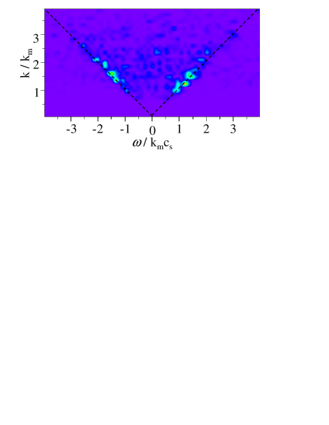
Figure 1: Density source power spectrum, $k^{4}|I(k,\omega)|^{2}$, with $\tilde{I}_{0}\simeq 4.12,\ \nu=0.15,\tilde{T}_{c}\simeq 0.033,$ and $k_{m}^{2}z/k_{0}\simeq 7.9.$ The dashed lines are at $\omega=\pm kc_{s}$.

The fraction of power in this acoustic peak, ${{\int\limits_{{{2kc_{s}}\mathord{\left/{\vphantom{{2kc_{s}}3}}\right.\kern-1.2pt}3}<\left|\omega\right|<{{4kc_{s}}\mathord{\left/{\vphantom{{4kc_{s}}3}}\right.\kern-1.2pt}3}}{\left|{I\left({k,\omega}\right)}\right|^{2}d\omega}}\mathord{\left/{\vphantom{{\int\limits_{{{2kc_{s}}\mathord{\left/{\vphantom{{2kc_{s}}3}}\right.\kern-1.2pt}3}<\left|\omega\right|<{{4kc_{s}}\mathord{\left/{\vphantom{{4kc_{s}}3}}\right.\kern-1.2pt}3}}{\left|{I\left({k,\omega}\right)}\right|^{2}d\omega}}{\int_{-\infty}^{+\infty}{\left|{I\left({k,\omega}\right)}\right|^{2}d\omega}}}}\right.\kern-1.2pt}{\int_{-\infty}^{+\infty}{\left|{I\left({k,\omega}\right)}\right|^{2}d\omega}}}\qquad,$ increases significantly as $\tilde{I}_{0}$ passes through its threshold value for a particular $k$, as shown in figure 2.

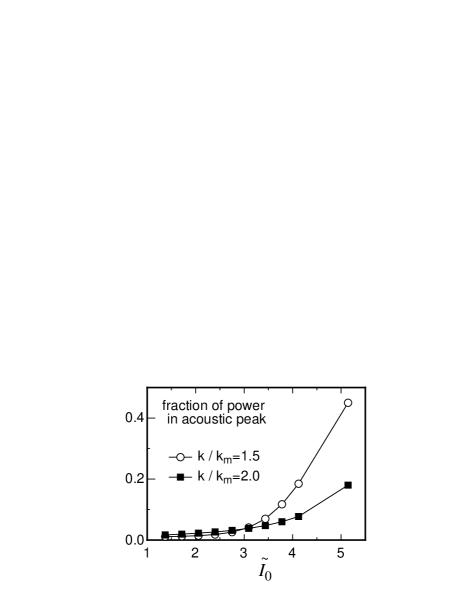
Figure 2: Fractional power in acoustic peak of the intensity fluctuation spectrum, with parameters as in figure 1, except $k_{m}^{2}z/k_{0}\simeq 5.2.$ Note that the FSBS intensity threshold for $k/k_{m}=$ 1.5 (2.0) is about 3 (4)

There is no discernible difference in shape between $|E(k,\omega,z)|^{2}$ at $z=0$, where it is $\propto 1/\big{[}1+(\omega T_{c})^{2}\big{]}$, and at finite $z$, for small $T_{c}$.

If $\tilde{\lambda}_{\max}\ll 1$, i.e., $\tilde{I}_{0}\lesssim 1,$ then the FSBS growth length, ${1\mathord{\left/{\vphantom{1{\lambda_{\max}}}}\right.\kern-1.2pt}{\lambda_{\max}}}$, is large compared to the (vacuum) $z$ correlation length, $\propto{{k_{0}}\mathord{\left/{\vphantom{{k_{0}}{k_{m}^{2}}}}\right.\kern-1.2pt}{k_{m}^{2}}}$, and it is found, for small $T_{c}$, that a quasi-equilibrium is attained: various low order statistical moments are roughly constant over the simulation range once $k_{m}^{2}z/k_{0}\gtrsim 5$, as seen in figure 3.

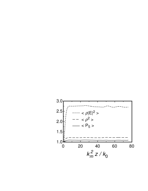
Figure 3: A quasi-equilibrium is attained with one point $E$ fluctuations remaining nearly Gaussian, as evidenced by the small change in $P_{5}$ StillBergerEtAl2000 , the fraction of power with intensity at least $5I_{0}$, but strongly modified $I-\rho$ correlations. Parameters are $\tilde{I}_{0}\simeq 0.53,\,\nu=0.3$ and $\tilde{T}_{c}\simeq 0.26$. Each curve is normalized to its value at z=0.

A true equilibrium cannot be attained since $\langle k^{2}\rangle\equiv\langle|\nabla E|^{2}\rangle/I_{0}$ grows due to scattering from density fluctuations as in figure 4.

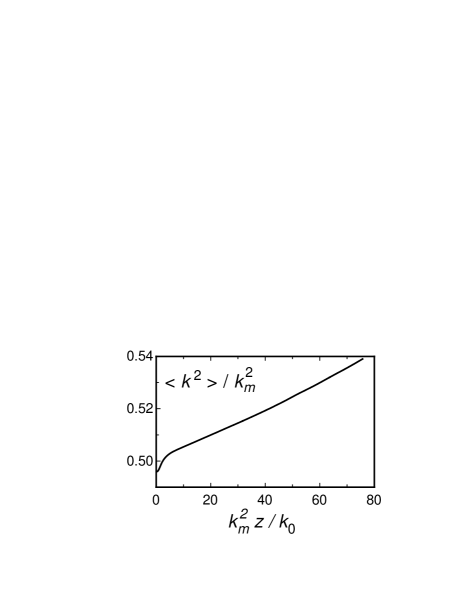
Figure 4: For parameters of figure 3, $\langle k^{2}\rangle\equiv\langle|\nabla E|^{2}\rangle/I_{0}$, increases little over the initial equilibration distance of roughly 5 in these units. The subsequent diffusion rate is 4.4E-04.

A dimensionless diffusion coefficient, $\tilde{D}\equiv(k_{0}/k_{m}^{4})\frac{d}{dz}\langle k^{2}\rangle,$ (proportional to the rate of angulare diffusion) may be extracted from the data of figure 4 by fitting a smooth curve to $\langle k^{2}\rangle$ for $5<k_{m}^{2}z/k_{0}<76$, and evaluating its slope, extrapolated to $z=0$. This yields a diffusion coefficient of 4.4E-04.

$\tilde{D}$ may be compared to the solution of the stochastic Schroedinger equation (SSE) BalRyzhik2002 with a self-consistent random potential Zakharov , $\rho$, whose covariance, $C^{\rho\rho}$ ($C^{\rho\rho}$ is a quadratic functional of $F(k)$) is evaluated as follows Moody2000 . Take $E$ as given by Eqn. $(\ref{Eeq1})$ with $\rho$ set to $0$ since it goes to zero with $\tilde{T}_{c}$, and use it in Eqn. $(\ref{neq1})$, with $\ln(1+\rho)\to\rho$, to evaluate $C^{\rho\rho}$. This is consistent only if $\tilde{I}_{0}<1,$ so that the density responce is stable except at small $k/k_{m}$. It follows, to leading order in $\tilde{T}_{c}$, that the SSE prediction for $\tilde{D},$ for the top hat spectrum,

$$\tilde{D}_{SSE}=\nu\tilde{T}_{c}\tilde{I}_{0}^{2}/68.8\ldots,$$ (10)

has the value 3.2E-04 for the parameters of Fig. 4. Note that $\tilde{D}_{SSE}$ is proportional to $\langle\rho^{2}\rangle$ and the roughly $20\%$ increase of $\langle\rho^{2}\rangle$ over its perturbative evaluation (see figure 3) used in the SSE accounts for about $1/2$ of the difference between $\tilde{D}$ and $\tilde{D}_{SSE}$.

We find that $\tilde{D}$ depends essentially on the spectral form, $\langle{|{\hat{E}(k)}|^{2}}\rangle=F(k)$ , e.g., for Gaussian $F(k)$ with the same value of $\langle k^{2}\rangle$, $D_{Gaussain}\approx 3D_{top\;hat}$. A numerical example of this dependence is found in figures 4 and 5. $\tilde{D}$ changes by $40\%$ over $5<k_{m}^{2}z/k_{0}<76$, because $F(k)$ changes significantly as seen in figure 5.

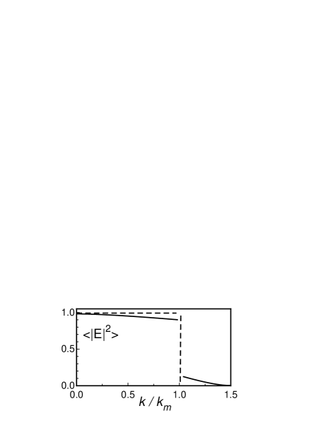
Figure 5: Top hat boundary condition, dashed line, changes qualitatively over the propagation distance shown in figure 4: solid line at $k_{m}^{2}z/k_{0}\simeq 76.$

In this sense, for NIF relevant boundary conditions, angular diffusion is an essential correction to the geometrical optics model, which (absent refraction) has constant $F(k)$.

Eqn. (10) implies that ${d\mathord{\left/{\vphantom{d{dz}}}\right.\kern-1.2pt}{dz}}\left\langle{\left({{k\mathord{\left/{\vphantom{k{k_{m}}}}\right.\kern-1.2pt}{k_{m}}}}\right)^{2}}\right\rangle\propto{1\mathord{\left/{\vphantom{1{k_{m}}}}\right.\kern-1.2pt}{k_{m}}}$, while $\lambda_{\max}\propto{1\mathord{\left/{\vphantom{1{k_{m}^{8}}}}\right.\kern-1.2pt}{k_{m}^{8}}}$. If the diffusion length is smaller than the FSBS growth length, then propagation, which effectively increases $k_{m}$, will reinforce this ordering. This stability condition may be expressed as $\tilde{D}>\tilde{\lambda}_{\max}$, or qualitatively as comment6

$$\nu\tilde{T}_{c}>\tilde{I}_{0}^{3}.$$ (11)

This is a global condition, as opposed to the wavenumber dependent threshold, $k_{cutoff}({\tilde{I}_{0}})$. However, even if Eqn. (11) is violated, it is not until $k_{cutoff}\approx 1.5k_{m}$, so that the peak of the density fluctuation spectrum is unstable, that FSBS has a strong effect. For these larger $I_{0}$ values a quasi-equilibrium is not attained, and it is more useful to consider an integral measure, $\triangle(\langle k^{2}\rangle,z)\equiv\langle k^{2}\rangle(z)-\langle k^{2}\rangle(0)$, of the change in beam angular divergence, rather than the differential measure, $D$. $\triangle/\tilde{I}_{0}^{2}$ is shown in Fig. 6, normalized to unity at $\tilde{I}_{0}=0.61$.

Note that we have not observed significant departure from Gaussian $E$ fluctuations for $\tilde{I}_{0}<2$ for the parameters of figure 6, which is consistent with the absence of self-focusing.

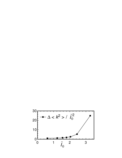
Figure 6: Beam angular divergence rate increases rapidly with $\tilde{I}_{0}$. $k_{m}^{2}z/k_{0}\simeq 15.7,$ $\nu=0.0375,\tilde{T}_{c}\simeq 0.125.$ In contrast, Eq. $(\ref{Deq1})$ predicts a flat curve around 1.

Therefore in this regime the effect of FSBS is benign, and perhaps useful for NIF design purposes: correlation lengths decrease, at an accelerated pace compared to SSE for $\tilde{I}_{0}\sim 1$, with $z$, while electric field fluctuations stay nearly Gaussian. As a result Afeyan , the intensity threshold for other instabilities (e.g., backscatter SBS) increases RoseDuBois1994 . If $\tilde{I}_{0}>4$, there are large non-Gaussian fluctuations of $E$, which indicates strong self-focusing.

In conclusion, well above the FSBS threshold we observe strong self-focusing effects, while well below threshold beam propagation is diffusive in angle with essential corrections to geometric optics. In an intermediate range of intensities the rate of angular diffusion increases with propagation. In the weak and intermediate regimes, the diffusion results in decreasing correlation lengths which could be beneficial for NIF.

One of the author (P.L.) thanks E.A. Kuznetsov for helpful discussions.

Support was provided by the Department of Energy, under contract W-7405-ENG-36.

References

(1) J.D. Lindl, Phys. Plasma 2, 3933 (1995).
(2)It is also assumed that intensity fluctuations which self-focus on a
time scale are not statistcally significant. See H. A. Rose and D. F. DuBois, Physics of Fluids
B5, 3337(1993).
(3)A. J. Schmitt and B. B. Afeyan, Phys. Plasmas 5, 503 (1998).
(4)C. H. Still, et al., Phys. Plasmas 7, 2023 (2000).
(5)R. H. Lehmberg and S. P. Obenschain, Opt. Commun. 46, 27 (1983).
(6) Fourier transform is in the plane with .
(7)This requires that the speed of light, ,
where is the correlation length.
(8)P. K. Kaw, G. Schmidt and T. W. Wilcox, Phys. Fluids 16,
1522 (1973).
(9)A. J. Schmitt and R. S. B. Ong, J. Appl. Phys 54, 3003 (1983).
(10)A. J. Schmitt, Phys. Fluids 31, 3079 (1988).
(11)H. A. Rose, D. F. DuBois and D. Russell,
Sov. J. Plasma Phys. 16, 537 (1990).
(12) D.N. Christodoulides, T.H. Coskun, M. Mitchell and M. Segev,
PRL 78, 646 (1997).
(13)The precise condition depends on : see
Ref. [11] and H. A. Rose and D. F. DuBois, Phys. Fluids B 4, 252 (1992). The first derivation
of an analogous result for the case of the modulational
instabiity of a broad Langmuir wave spectrum was done
by A. A. Vedenov and L. I. Rudakov, Soviet Physics Doklady 9, 1073 (1965); Doklady Akademii Nauk SSR 159, 767 (1964).
(14)If is constrained by finite beam size effects to be, , (beam diameter),
then stability is regained for small enough .
(15)See, , G. Bal, G. Papanicolaou and L. Ryzhik, Nonlinearity 15, 513 (2002).
(16)This may be viewed as a special case of the wave kinetic Eq. [see e.g.
V.E. Zakharov, V.S. Lvov, and G. Falkovich, Kolmogorov
Spectra of Turbulence I: Wave turbulence (Springer-Verlag, New
York, 1992)].
(17)It is assumed that the density fluctuations are only due to the beam itself, in contrast to
the experimental configuration found in J. D. Moody, et al., Phys. Plasma 7, 2114 (2000).
(18)If collisonal absorption is included in Eq. (3), with rate , then for , the
stability condition is .
(19)B. Afeyan (private comm. 2003) has reached somewhat similar conclusions in the context of self-focusing.
(20)H. A. Rose and D. F. DuBois, Phys. Rev. Lett. 72, 2883 (1994).