Challenges in Moving the LEP Higgs Statistics to the LHC

Abstract

We examine computational, conceptual, and philosophical issues in moving the statistical techniques used in the LEP Higgs working group to the LHC.

I Introduction

Higgs searches at LEP were based on marginal signal expectations and small background uncertainties. In contrast, Higgs searches at the LHC are based on strong signal expectations and relatively large background uncertainties. Based on our experience with the LEP Higgs search, our group tried to move the tools we had developed at LEP to the LHC environment. In particular, our calculation of confidence levels was based on an analytic computation with the Fast Fourier Transform and the log-likelihood ratio as a test statistic (and systematic errors based on the Cousins-Highland approach). We encountered three types of problems when calculating ATLAS’ combined sensitivity to the Standard Model Higgs Boson: problems associated with large numbers of expected events, problems arising from very high significance levels, and problems related to the incorporation of systematic errors.

Previously, it was shown that the migration of the statistical techniques that were used in the LEP Higgs Working Group to the LHC environment is not as straightforward as one might naïvely expect UW-confidence-VBF . After a brief overview in Section II, those difficulties and their ultimate solution are discussed in Section III. Our group has developed two independent software solutions (both in C++; both with FORTRAN bindings; one ROOT based and the other standalone) which can be found at:

http://wisconsin.cern.ch/software

In Section IV we discuss the incorporation of systematic errors and compare a few different strategies. In Section V we present and discuss the discovery luminosity (the luminosity expected to be required for discovery). Lastly, in Section  VI we discuss the statistical notion of power (which is related to the probability of Type II error (the probability we do reject the “signal-plus-background hypothesis” when it is true).

II The Formalism

Our starting point for this note is a brief review of the techniques that were used at LEP. We refer the interested reader to Kendall for an introduction to the fundamentals, to Read:1997 for why the likelihood ratio has been chosen as a test statistic, to Junk:1999kv for a Monte Carlo approach to the calculation and to clfft for the analytic calculation using Fast Fourier Transform (FFT) techniques. For completeness, we introduce the basic approach below using the notation found in UW-confidence-VBF . For a counting experiment where we expect, on average, $b$ background events and $s$ signal events, we consider two hypotheses: the null (or background-only) hypothesis in which the number of expected events, $n$, is described by a Poisson distribution $P(n;b)$ and the alternate (or signal-plus-background) hypothesis in which the number of expected events is described by a Poisson distribution $P(n;s+b)$. Here the number of events serves the purpose of a test statistic: a real number which quantities an experiment.

It is possible to include a discriminating variable $x$ which has some probability density function (pdf) for the background, $f_{b}(x)$, and some pdf for the signal, $f_{s}(x)$, both normalized to unity. Given an observation at $x$ we can construct the Likelihood Ratio $Q=(sf_{s}(x)+bf_{b}(x))/bf_{b}(x)$. With several independent observations $\{\hat{x}_{i}\}$ we can consider the combined likelihood ratio $Q=\prod Q_{i}$ . It is possible, and in some sense optimal, to use $Q$ (or in practice $q=\ln Q$) as a test statistic.

The computational challenge of using the log-likelihood ratio in conjunction with a discriminating variable $x$ is the construction of the log-likelihood ratio distribution for the background-only hypothesis, $\rho_{b}(q)$, and for the signal-plus-background hypothesis $\rho_{s+b}(q)$. In this case, there are not only the Poisson fluctuations of the number of events, but also the continuously varying discriminating variable $x$. In particular, for a single background event the log-likelihood ratio distribution, $\rho_{1,b}(q)$, must incorporate all possible values of $x$. From these single event distributions we can build up the expected log-likelihood ratio distribution by repeated convolution. This is most effectively done by using a Fast Fourier Transform (FFT) where convolution can be expressed as multiplication in the frequency domain (denoted with a bar). In particular we arrive at:

$$\overline{\rho_{b}(q)} = e^{b[\overline{\rho_{1,b}(q)}-1]}\hskip 14.45377pt{\rm and}$$ (1)

$$\overline{\rho_{s+b}(q)} = e^{(s+b)[\overline{\rho_{1,s+b}(q)}-1]}.$$

From the log-likelihood distribution of the two hypotheses we can calculate a number of useful quantities. Given some experiment with an observed log-likelihood ratio, $q^{*}$, we can calculate the background-only confidence level, $CL_{b}$ :

$$CL_{b}(q^{*})=\int_{q^{*}}^{\infty}\rho_{b}(q^{\prime})dq^{\prime}$$ (2)

In the absence of an observation we can calculate the expected $CL_{b}$ given the signal-plus-background hypothesis is true. To do this we first must find the median of the signal-plus-background distribution $\overline{q}_{s+b}$. From these we can calculate the expected $CL_{b}$ by using Eq. 2 evaluated at $q^{*}=\overline{q}_{s+b}$.

Finally, we can convert the expected background confidence level into an expected Gaussian significance, $N\sigma$, by finding the value of $N$ which satisfies

$$CL_{b}(\overline{q}_{s+b})=\frac{1-{\rm erf}(N/\sqrt{2})}{2}.$$ (3)

where ${\rm erf}(N)=(2/\pi)\int_{0}^{N}\exp(-y^{2})dy$ is a function readily available in most numerical libraries.

III Numerical Difficulties

The methods described in the previous section have been applied to the combined ATLAS Higgs effort with some caveats related to numerical difficulties UW-confidence-VBF . In particular, in the extreme tails of $\rho_{b}(q)$, the probability density is dominated by numerical noise. This numerical noise is an artifact of round-off error in the double precision numbers used in the Fast Fourier Transform. The noise is on the order of $10^{-17}$ (for double precision floating point numbers), which translates into a limit on the significance of about $8\sigma$. For particular values of the Higgs mass, ATLAS has an expected significance well above $8\sigma$ with only $10~{}\rm fb^{-1}$ of data. In order to produce significance values above the $8\sigma$ limit, various extrapolation methods were used in UW-confidence-VBF . We now introduce a definitive solution to this problem based on arbitrary precision floating point numbers.

It should be made clear that the numerical precision problem is not due to the fact that the $CL_{b}$ is so small that the evaluation of the integral in Eq. 2 cannot be treated with double precision floating point numbers. Instead, the numerical precision problem is due to the many (approximately $2^{20}$) Fourier modes which must in total produce a number very close to $0$. In order to rectify this problem we have implemented the Fast Fourier Transform with the arbitrary-precision floating point numbers provided in the CLN library GiNaC . One might protest that above $5\sigma$ we are not interested in the precise value of the significance and that this exercise is purely academic. We refer the interested reader to Sections V &  VI for different summaries of an experiments discovery potential.

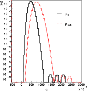
Figure 1: The distribution of the log-likelihood ratio $\rho(q)$ for the null and alternate hypothesis (the axis labels refer to bins of $q$, not $q$ itself). For $q>10^{5}$ the distribution is contaminated by numerical noise (see text for details).

III.1 Extrapolation

While the arbitrary precision FFT approach is the definitive solution to the problem of calculating very high expected significance, it is also incredibly time consuming. A much faster, approximate solution is to approximate the $CL_{b}$ by fitting the $\rho_{b}$ distribution to a functional form. The first method of extrapolation studied was a simple Gaussian fit to the $\rho_{b}$ distribution. This method works fairly well, but tends to overestimate the significance. The second method we studied was based on a Poisson fit to the $\rho_{b}$ distribution. The Poisson distribution has the desirable properties that it will have no probability below the hard limit $q\geq-s$ and that its shape is more appropriate UW-confidence-VBF . Figure 2 compares these different extrapolation methods.

IV Incorporating Systematic Uncertainty

One encounters both philosophical and technical difficulties when one tries to incorporate uncertainty on the predicted values $s$ and $b$ found in Eq. 1. In a Frequentist formalism the unknown $s$ and $b$ become nuisance parameters. In a Bayesian formalism, $s$ and $b$ can be marginalized by integration over their respective priors. At LEP the practice was to smear $\rho_{b}$ and $\rho_{s+b}$ by integrating $s$ and $b$ with a multivariate normal distribution as a prior. This smearing technique is commonly referred to as the Cousins-Highland Technique, and it is has some Bayesian aspects.

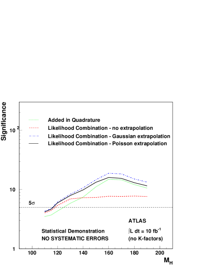
Figure 2: Comparison of the ATLAS Higgs combined significance obtained from several approximate techniques. The (red) dashed line corresponds to the unmodified likelihood ratio which can not produce significance values above about $8\sigma$ (see text). This figure is meant to demonstrate the different methods of combination and does not include up-to-date results from the various Higgs analyses.

IV.1 A Purely Frequentist Technique

At the PhysStat2003 conference a purely frequentist approach to hypothesis testing with background uncertainty was presented Cranmer2003freq . This method relies on the full Neyman construction and uses a likelihood ratio similar to the profile method as an ordering rule. In this formalism, a systematic uncertainty at the level of 10% has a much larger effect than when treated with the Cousins-Highland technique.

IV.2 The Cousins Highland Technique

The Cousins-Highland formalism for including systematic errors on the normalization of the signal and background is provided in Cousins:1992qz and generalized in Junk:1999kv ; clfft . In particular, for a multivariate normal distribution as a prior for the $n_{i}$ the distribution of the log-likelihood ratio is given by:

$$\overline{\rho_{sys}(q)}=\int...\int e^{\sum_{i}^{K}n_{i}[\overline{\rho_{1,i}(q)}-1]}\left(\frac{1}{\sqrt{2\pi}}\right)^{K}\frac{1}{\sqrt{|S|}}$$ (4)

$$e^{\sum_{i}^{K}\sum_{j}^{K}-\frac{1}{2}(n_{i}-\langle n_{i}\rangle)S^{-1}_{ij}(n_{j}-\langle n_{j}\rangle)}\prod_{i}dn_{i}$$

where $S_{ij}=\langle(n_{i}-\langle n_{i}\rangle)(n_{j}-\langle n_{j}\rangle)\rangle$. Reference clfft provides an analytic expression for the resulting log-likelihood ratio distribution including a correlated error matrix; however, this equation was obtained with an integration over negative numbers of expected events and does not hold. Attempts to provide a closed form solution for the positive semi-definite region require analytical continuation of the error function over a wide range of the complex plane. Instead, a numerical integration over the positive semi-definite region has been adopted for our software packages.

V Discovery Luminosity

Because the calculation of expected significance is technically very difficult at the LHC, other summaries of the discovery potential have been explored. While these techniques are not new, it is important to consider their pros and cons. One such alternate summary of the discovery potential is based on the discovery luminosity”. Define the discovery luminosity, $L^{*}(m_{H})$, to be the integrated luminosity necessary for the expected significance to reach $5\sigma$. The discovery luminosity is an informative quantity; however, it must be interpreted with some care:

• Collecting an integrated luminosity equal to the nominal discovery luminosity does not guarantee that a discovery will be made. Instead, with $L^{*}(m_{H})$ of data the median of $\rho_{s+b}$ will be at the $5\sigma$ level – which corresponds to a 50% chance of discovery. See Section VI for more details.

• In practice an analysis’ cuts, systematic error, and signal and background efficiencies are luminosity-dependent quantities. When we calculate the discovery luminosity, we treat the analysis as constant.

VI The Power of a $\bf 5\sigma$ Test

The traditional quantity which is used to summarize an experiment’s discovery potential is the combined significance; however, as was noted in Section III this plot becomes very dificult to make when the significance goes beyond about $8\sigma$. Furthermore, the plot itself starts to loose relevance when the significance is far above $5\sigma$. The discovery luminosity is another possible way of illustrating an experiment’s discovery potential, but it must be interpreted with some care. A third summary of an experiment’s discovery potential which is related to the probability of Type II error: the power. First, it should be noted that the expected significance is a measure of separation between the medians of the background-only and signal-plus-background hypotheses. Thus, when we see the significance curve cross the $5\sigma$ line in Fig. 2 there is only a 50% chance that we would observe a $5\sigma$ effect if the Higgs does indeed exist at that mass. In practice, we claim a discovery if the observed data exceeds the $5\sigma$ critical region, and do not claim a discovery if it doesn’t. The meaning of the $5\sigma$ discovery threshold is a convention which sets the probability of Type I error to be $2.85\cdot 10^{-7}$ . With that in mind, the idea that the significance is $20\sigma$ at $m_{H}=160~{}{\rm GeV}$ is irrelevant. What is relevant is the probability that we will claim discovery of the Higgs if it is indeed there: that quantity is called the power. The power is defined as $1-\beta$ where $\beta$ is the probability of Type II error: the probability that we reject the signal-plus-background hypothesis when it is true Kendall .

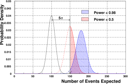
Figure 3: Examples of power for two different signal-plus-background hypotheses with respect to a single background-only hypothesis with 100 expected events (black).

Consider Figure 3 with a background expectation of 100 events. The black vertical arrow denotes the $5\sigma$ discovery threshold. The (red) dashed curve shows the distribution of the number of expected events for a signal-plus-background hypothesis with 150 events. Normally, we would say the expected significance is $5\sigma$ for this hypothesis; however, we can see that only 50% of the time we would actually claim discovery. The rightmost (blue) curve shows the distribution of the number of expected events for a signal-plus-background hypothesis with 180 events. Normally, we would say the expected significance is $8\sigma$ for this hypothesis; however, a more meaningful quantity – the power – is associated with the probability we would claim discovery which is about 98%. In addition to the power being a germane quantity, it is much easier to calculate.

VII Conclusion

In conclusion, the migration of the statistical tool-set developed at LEP to the LHC environment is not as straightforward as one might expect. The first difficulties are computational and arise from the combination of channels with many events and channels with few events (these are easily solved). The next difficulties are numerical and arise from the extremely high expected significance of the high-energy frontier. These problems can be solved by brute force; or they can be reinterpreted as conceptual problems, and solved by asking different questions (i.e. power). Lastly, there is a philosophical split related to the Bayesian and Frequentist approach to uncertainty. At the LHC, the choice of the formalism is no longer a second-order effect, and this problem is not so easy to solve.

- [1] K.S. Cranmer et. al. Confidence level calculations for for using vector boson fusion. ATLAS communication ATL-COM-PHYS-2002-049 (2002).
- [2] J.K Stuart, A. Ord and S. Arnold. Kendall’s Advanced Theory of Statistics, Vol 2A (6th Ed.). Oxford University Press, New York, 1994.
- [3] A.L. Read. Optimal statistical analysis of search results based on teh likelihood ratio and its application to the search for the MSM higgs boson at 161 and 172 GeV. DELPHI note 97-158 PHYS 737 (1997).
- [4] T. Junk. Confidence level computation for combining searches with small statistics. Nucl. Instrum. Meth., A434:435–443, 1999.
- [5] J. Nielsen H. Hu. Analytic confidence level calculations using the likelihood ratio and fourier transform. “Workshop on Confidence Limits”, Eds. F. James, L. Lyons and Y. Perrin, CERN 2000-005 (2000), p. 109.
- [6] C. Bauer et. al. Introduction to the GiNaC framework for symbolic computation within the c++ programing language. J. Symbolic Computation, 33:1–12, 2002.
- [7] K.S. Cranmer. Frequentist hypothesis testing with background uncertainty., 2003. “PhyStat2003”, SLAC. physics/0310108.
- [8] R.D. Cousins and V.L. Highland. Incorporating systematic uncertainties into an upper limit. Nucl. Instrum. Meth., A320:331–335, 1992.