Electromagnetic transitions of the helium atom in superstrong magnetic fields

Abstract

We investigate the electromagnetic transition probabilities for the helium atom embedded in a superstrong magnetic field taking into account the finite nuclear mass. We address the regime $\gamma=100-10\ 000$ a.u. studying several excited states for each symmetry, i.e. for the magnetic quantum numbers $0,-1,-2,-3$, positive and negative z parity and singlet and triplet symmetry. The oscillator strengths as a function of the magnetic field, and in particular the influence of the finite nuclear mass on the oscillator strengths are shown and analyzed.

I Introduction

Exposing matter to strong and superstrong magnetic fields (which are fields of the order of $10^{5}$ T and above) dramatically changes its properties and yields new and unexpected phenomena. On the microscopic scale, i.e. for atomic and molecular systems, magnetic forces have a tremendous influence on the electronic structure and quantum dynamics Friedrich and Wintgen (1989); Ruder et al. (1994); Schmelcher and Schweizer (1998). This is due to the different appearances of the Coulomb and magnetic forces. From a theoretical point of view, strong and superstrong magnetic fields are interesting, because the competing forces prevent a perturbative treatment of the problem. Therefore it is necessary to develop and apply new nonperturbative techniques.

Certain astrophysical objects possess strong and superstrong magnetic fields Angel (1978); Pavlov et al. (1995); Wickramasinghe and Ferrario (2000). Atmospheres of magnetic white dwarfs are exposed to fields of the order of 100 – 10⁵ T, magnetic fields in the photosphere of neutron stars are of the order of 10⁵ –10¹⁰ T. For the interpretation of the spectra of these astrophysical objects a wealth of highly accurate atomic and molecular energies, transition wavelengths and transition probabilities are needed. An example for the analysis of astrophysical spectra of magnetized objects using atomic data in strong fields is the white dwarf GrW$+70^{\circ}8247$, which represents a cornerstone for the understanding of magnetic white dwarfs in general Angel et al. (1985); Greenstein et al. (1985); Wunner et al. (1985); Wickramasinghe and Ferrario (1988).

Highly accurate data are available for hydrogen in strong magnetic fields since more than a decade Friedrich and Wintgen (1989); Ruder et al. (1994); Kravchenko et al. (1996). This system is now understood to a very high degree. However beyond hydrogen, there is significant interest in detailed data on heavier elements, such as He, Na, Fe and even molecules. Especially helium plays an important role in the atmospheres of magnetic white dwarfs and potentially also neutron stars. The electronic structure of the helium atom has been considered by several authors during the last decades Mueller et al. (1975); Virtamo (1976); Pröschl et al. (1982); Vincke and Baye (1989); Braun et al. (1993); Ivanov (1994); Thurner et al. (1993); Braun et al. (1998); Heyl and Hernquist (1998). However most of the corresponding investigations are restricted to a few states or field strengths. Only a few works provide accuracies, that are necessary for astrophysical applications.

Recently detailed investigations of helium in the strong field regime have been performed, providing the community with detailed energy levels, transition wavelengths, and transition probabilities, for a dense grid of field strengths in the range of $0\leq\gamma\leq 100$ a.u. (one atomic units corresponds to $2.3505$ $\times$ $10^{5}$ T) Becken et al. (1999); Becken and Schmelcher (2000, 2001, 2002). Numerous symmetries and many excited states have been addressed. With the resulting large amount of data it was possible to identify the absorption edges of the observational spectrum of the magnetic white dwarf GD229 Green and Liebert (1980); Schmidt et al. (1990, 1996), which have been unexplained for more than 25 years Jordan et al. (1998, 2001).

At this point also the work by Jones et. al Jones et al. (1999) should be mentioned. They applied a released-phase quantum Monte Carlo method in order to evaluate bound state energies and dipole-matrix elements for the ground and a few excited triplet states. This has been done for a grid of several field strengths $0.08\leq\gamma\leq 800$ a.u.

Addressing the superstrong field regime a further challenge is the problem of the finite nuclear mass. The dominant energy correction, caused by the finite nuclear mass is for a field of $10^{9}$ T of the same order of magnitude as the binding energy itself. This holds even for the energetically lowest states Al-Hujaj and Schmelcher (2003). Therefore effects due to the finite nuclear mass have to be taken into account for a correct description of the structure of the atom. Up to date there are no detailed studies about the influence of the finite nuclear mass on the transition rates.

The purpose of the present article is to provide results on the transition probabilities for helium in the superstrong field regime. In Sect. II we review the expressions for the transition matrix elements and analyze the influence of the finite nuclear mass. In Sect. III we provide our results and discuss some particular features of the transition probabilities as a function of the field strength. Sect. IV provides a brief conclusion and an outlook.

II Electromagnetic transition probabilities for finite nuclear mass

A detailed comparison of theoretical and observational spectra requires not only the energies and transition wavelengths, but also the corresponding oscillator strengths. Selection rules of allowed and forbidden transitions are of particular importance. Our investigation focuses on the dominant electric dipole transitions. We will shortly review the derivation of the corresponding operators since there are modifications due to the presence of the magnetic field as well as the finite nuclear mass.

Our starting point is the pseudo-separated Hamiltonian W. E. Lamb (1952); Avron et al. (1978); Johnson et al. (1983); Schmelcher et al. (1994) using relative coordinates $\{\bm{r}_{i}\}$ for the electrons with respect to the nucleus in atomic units:

$$H = \sum_{i}\left\{\frac{1}{2}\left(\frac{\bm{P}}{M_{A}}+\bm{p}_{i}+\frac{1}{2}\bm{B}\times\bm{r}_{i}\right)^{2}-\frac{2}{|\bm{r}_{i}|}\right\}$$ (1)

$$+ \frac{1}{2M_{0}}\left(\frac{M_{0}}{M_{A}}\bm{P}-\sum_{j}\bm{p}_{j}+\frac{1}{2}\sum_{j}\bm{B}\times\bm{r}_{j}\right)^{2}$$ (2)

$$+ \frac{1}{|\bm{r}_{1}-\bm{r}_{2}|}$$ (3)

Here is $M_{A}$ the total mass of the atom, $\bm{P}$ denotes the pseudo-momentum, and $\bm{B}$ the magnetic field vector.

On the other hand, we have the operator $H_{rad}$ describing the interaction of the system with the electromagnetic radiation field $\bm{A}_{r}$, neglecting quadratic terms in $\bm{A}_{r}$. It is given in relative coordinates by

$$H_{rad} = \sum_{i}\left(\frac{1}{M_{A}}\bm{P}+\bm{p}_{i}+\frac{1}{2}\bm{B}\times\bm{r}_{i}\right)\bm{A}_{r}(\bm{r}^{\prime}_{i})+$$ (5)

$$-\frac{2}{M_{0}}\sum_{i}\left(\frac{M_{0}}{M_{A}}\bm{P}-\sum_{j}\left(\bm{p}_{j}-\frac{\bm{B}\times\bm{r}_{j}}{2}\right)\right)\bm{A}_{r}(\bm{r}^{\prime}_{N}).$$

Here $\bm{r}^{\prime}_{i}$ denotes the position vector of electron $i$ and $\bm{r}^{\prime}_{N}$ the position of the nucleus in the laboratory frame. The radiative part of the electromagnetic field $\bm{A}_{r}(\bm{r})$ reads in quantized form (we consider only the creation of photons):

$$\bm{A}_{r}(\bm{r})=\sum_{\bm{k},\lambda}N(\bm{k})a^{+}_{\bm{k},\lambda}\bm{\epsilon}_{\bm{k},\lambda}\exp(i\bm{k}\bm{r}+i\omega t)$$ (6)

$a^{+}_{\bm{k},\lambda}$ denotes the creation operator for a photon with wave vector $\bm{k}$ and wavelength $\lambda$. $\bm{\epsilon}_{\bm{k},\lambda}$ is the polarization vector of the photon, whereas $N$ is an amplitude. In the next step, we will integrate over the center of mass coordinate $\bm{R}$ by calculating the matrix element of $H_{rad}$ between two eigenfunctions of the pseudo-momentum $\bm{P}$ (eigenvalues are denoted by $\bm{K_{i}}$ and $\bm{K_{f}}$), which are given by expressions of the form:

$$\frac{1}{\sqrt{V}}\exp\left(-i\bm{K}\cdot\bm{R}\right)$$ (7)

if we assume an integration volume $V$.

The dipole approximation, which reads $\exp(i\bm{k}\cdot\bm{r}_{i})\approx 1$, leads us in first order time dependent perturbation theory to the following expression for the transition rates:

$$\frac{dP_{fi}}{dt} = 2\pi\sum_{\sigma}\left[\delta(E_{f}-E_{i}-\omega)\delta_{\bm{K}_{i},\bm{K}_{f}-\bm{k}}\times\right.$$ (9)

$$\left.\left|<i|\bm{G_{\sigma}^{+}}|f>\right|^{2}\right]$$

where

$$\bm{G_{\sigma}^{+}}=-N(\bm{k})a^{+}_{\sigma}\bm{\epsilon}_{\sigma}^{*}\sum_{i}\left(\frac{M_{A}}{M_{0}}\bm{p}_{i}+\frac{M_{0}-2}{2M_{0}}\bm{B}\times\bm{r}_{i}\right),$$ (10)

and $<i|$, $|f>$, denote the electronic initial and final states, respectively. In the following we will assume that the wavevector $\bm{k}$ is much smaller than $\bm{K}_{i},\bm{K}_{f}$, which is well-justified in atomic transitions. Thus using $\bm{\epsilon}_{\sigma}^{*}(\frac{M_{A}}{M_{0}}\bm{p}+\frac{M_{0}-2}{2M_{0}}\bm{B}\times\bm{r})=:Q_{\sigma}$, we obtain the following expressions for the electronic transitions:

$$p_{fi}^{\sigma} = \frac{2}{E_{f}-E_{i}}<f|Q_{\sigma}|i>,$$ (11)

$$d_{fi}^{(\sigma)} = \left(\frac{2}{E_{f}-E_{i}}\right)^{2}|<f|Q_{\sigma}|i>|^{2},$$ (12)

$$f_{fi}^{(\sigma)} = \frac{E_{f}-E_{i}}{2}d_{fi}^{(\sigma)}.$$ (13)

These expressions represent the dipole-matrix element, the dipole strength and the oscillator strength, respectively in the velocity representation.

On the other hand we have for the expectation value of the commutator

$$<i|[H,\bm{r}]|f> = <i|\frac{M_{A}}{M_{0}}\bm{p}+\frac{M_{0}-2}{2M_{0}}\bm{B}\times\bm{r}|f>$$ (14)

$$= (E_{i}-E_{f})<i|\bm{r}|f>,$$ (15)

where $\bm{r}:=\bm{r}_{1}+\bm{r}_{2}$ and $\bm{p}:=\bm{p}_{1}+\bm{p}_{2}$ are symmetrized one-particle operators. Applying the identity of Eqs. (14),(15) we arrive at the length representation, that reads,

$$p_{fi}^{\sigma} = 2<f|D_{\sigma}|i>,$$ (16)

$$d_{fi}^{(\sigma)} = 4|<f|D_{\sigma}|i>|^{2},$$ (17)

$$f_{fi}^{(\sigma)} = \frac{E_{f}-E_{i}}{2}d_{fi}^{(\sigma)},$$ (18)

where $\bm{\epsilon}_{\sigma}^{*}\bm{r}=:D_{\sigma}$. These above two representations are equivalent. However in case of numerical calculations, the two representations yield in general different results. The relative deviation between the two representations is a good measure for the convergence of the computational method. Only results that obey certain consistency criteria concerning the length to velocity representations of the transition rates are presented. This ensures in particular the gauge independence of our results.

In the following we will assume a vanishing pseudo-momentum $\bm{K}$, which is an appropriate approximation in case of slow moving atoms. The basic polarization vectors $\bm{\epsilon}_{\sigma}$ are chosen to be parallel and perpendicular to the magnetic field vector, indicated as components $z$ and $x\pm iy$. This leads to the following selection rules for the electromagnetic transitions of the helium atom in a magnetic field Becken (2000):

$$|M_{f}-M_{i}|=1 \Pi_{z_{f}}\Pi_{z_{i}}=1,$$ and (19)

or

$$|M_{f}-M_{i}|=0 \Pi_{z_{f}}\Pi_{z_{i}}=-1$$ and (20)

and

$$S_{f}-S_{i}=0 S_{z_{f}}-S_{z_{i}}=0.$$ and (21)

Here Eq. (19), (20) describe circular and linear polarized transitions, respectively.

To understand the influence of the finite nuclear mass we rewrite the expression for the oscillator strength in the velocity form Eq. (18) as

$$f_{fi}^{(\sigma)}=2\left(E_{f}-E_{i}\right)|<f|D_{\sigma}|i>|^{2}.$$ (22)

The energy factor $(E_{f}-E_{i})$ plays a significant role, as we will see below. One result of Ref.Al-Hujaj and Schmelcher (2003) is, that effects of the mass polarization operators are small and therefore in a good approximation results for finite nuclear mass can be expressed in terms of results for infinite nuclear mass:

$$E(M_{0},\gamma)\approx\frac{1}{\mu^{\prime}}E(\infty,\gamma)-\frac{\gamma M}{M_{0}}+\frac{2\gamma}{M_{0}}\frac{\partial}{\partial\gamma}E(\infty,\gamma)$$ (23)

Here $E(M_{0},\gamma)$ denotes the total energy of an eigenstate for the Hamilton operator of the helium atom for nuclear mass $M_{0}$ and a field strength $\gamma$. $\mu^{\prime}:=(1-1/M_{0})^{-1}$ is a reduced mass. First we will concentrate on transitions which do not involve tightly bound states. For the corresponding transitions the last, i.e. third term on the right hand side of Eq. (23) in general cancels in the energy factor of Eq. (22). As a consequence, there are two generic cases (no tightly bound states involved) for the influence of the energy factor $(E_{f}-E_{i})$: In the case of linear polarized transitions, the magnetic quantum numbers $M_{i}$ and $M_{f}$ are equal and therefore the energy factor is just scaled by the factor $1/\mu^{\prime}$, compared to the results for an infinite nuclear mass. Typically these oscillator strengths are approximately constant as a function of the field strength. Note that the factor $1/\mu^{\prime}$ deviates for helium about $10^{-4}$ from 1. In the case of circular polarized transitions the second term on the r.h.s. of Eq. (23) $(-\gamma M/M_{0})$ becomes important, since the magnetic quantum numbers $M_{i}$ and $M_{f}$ are different. Therefore the linear term $\gamma/M_{0}$ is added to the energy factor, which in general causes an increase of the oscillator strengths compared to results for infinite nuclear mass, of the form

$$f_{fi}^{\sigma}(M_{0},\gamma)\approx\frac{1}{\mu^{\prime}}f_{fi}^{\sigma}(\infty,\gamma)+\frac{\gamma}{2M_{0}}|p^{\sigma}_{fi}(\infty,\gamma)|^{2}.$$ (24)

However, the typical oscillator strengths for circular polarized transitions decrease according to a power law. We note that in case of transitions emanating from tightly bound states the third term on the r.h.s. of Eq. (23) becomes important and in general modifies the pattern for linear polarized transitions. This is essentially due to the fact that the energies of magnetically tightly bound states exhibit an inherently different field dependence than the corresponding quantity of non tightly bound states. The above discussed behavior will be observed when discussing our results of oscillator strengths in Sect.III.

Some comments on our computational approach are in order. The calculations are performed using an anisotropic Gaussian basis set, which was put forward by Schmelcher and Cederbaum Schmelcher and Cederbaum (1988), and which has been successfully applied to several atoms, ions and moleculesKappes and Schmelcher (1996); Detmer et al. (1997, 1998); Becken et al. (1999); Becken and Schmelcher (2000, 2001, 2002); Al-Hujaj and Schmelcher (2000, 2003). The corresponding basis functions have been optimized for each field strength to solve the one particle problems, i.e. H and He⁺ in a magnetic field. We refer the reader to Ref.Al-Hujaj and Schmelcher (2003) for more details. It has been shown, that this approach yields accurate energies and in particular oscillator strength for helium, by comparing with the corresponding data in the literature Becken et al. (1999); Becken and Schmelcher (2000, 2001, 2002).

III Results

In this section, we present and discuss our results on the oscillator strengths of electric dipole transitions of helium in the superstrong field regime. In order to label the states, we use the standard spectroscopic notation $n^{2S+1}M^{\Pi_{z}}$. Here $2S+1$ indicates the spin multiplicity, $M$ is the magnetic quantum number, $\Pi_{z}$ the z parity, and $n$ the degree of excitation in the corresponding symmetry subspace. The accuracy for the reported oscillator strengths is between $10^{-4}$ and a few times $10^{-2}$.

As discussed in Ref.Al-Hujaj and Schmelcher (2003) the number of bound states of the helium atom in superstrong magnetic fields becomes finite, i.e. the spectrum terminates, if the effects of the finite nuclear mass are taken into account. Therefore only a finite, usually small number of transitions “survive” in the superstrong field regime. On the other hand the ionization threshold (He $\rightarrow$ He⁺ $+$ e^-) is up to date not known exactly due to missing detailed investigations on the moving He⁺ ion in a magnetic field. The exact field strength for which a certain state becomes unbound is therefore unknown. Since our basis functions cannot properly describe the electronic continuum we report here only on transitions that are known to be energetically well-separated enough from the continuum.

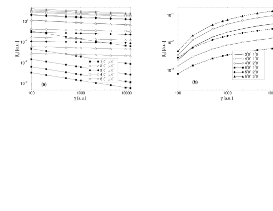
Figure 1: The absolute value of the oscillator strength $|f_{fi}|$ of the linear polarized transitions $\nu^{1}0^{+}\rightarrow\mu^{1}0^{-}$ as a function of the field strength $\gamma$. (a) On the left hand side from bottom to top $(\nu,\mu)$=$(5,4)$, $(5,5)$, $(4,3)$, $(4,4)$, $(3,2)$, $(3,3)$, $(2,2)$, $(2,1)$, $(4,5)$, $(1,1)$, $(3,5)$, $(2,4)$, $(1,2)$, $(2.5)$, $(1,3)$,$(1,4)$, $(1,5)$. (b) Oscillator strengths of a group of transitions belonging to these symmetry subspaces showing a different field dependency.

The typical features of oscillator strengths of linear polarized transition, discussed in Sect.II, can be clearly seen in Fig. 1 (a). The oscillator strengths for several transitions stay constant, or change much less than one order of magnitude. On the other hand transitions emanating from the tightly bound state $1^{1}0^{+}$ can be identified by their power law behavior. A completely different pattern belongs to the transitions $3^{1}0^{+}\rightarrow 1^{1}0^{-}$,$4^{1}0^{+}\rightarrow 1^{1}0^{-}$,$4^{1}0^{+}\rightarrow 2^{1}0^{-}$,$5^{1}0^{+}\rightarrow 1^{1}0^{-}$,$5^{1}0^{+}\rightarrow 1^{2}0^{-}$, and $5^{1}0^{+}\rightarrow 3^{1}0^{-}$, depicted in Fig. 1 (b). For a field strength below a critical field strength $\gamma_{c}\approx 50$ they decrease (this can not be seen in Fig. 1 (b)), above $\gamma_{c}$ they increase. Numerical values for transition wavelengths and oscillator strengths for a few of the lowest linear polarized transitions $\mu^{2S+1}0^{+}\rightarrow\nu^{2S+1}0^{-}$, $\mu,\nu=1,2$ are presented in table 1.

	$1^{1}0^{+}\rightarrow 1^{1}0^{-}$		$2^{1}0^{+}\rightarrow 1^{1}0^{-}$		$2^{1}0^{+}\rightarrow 2^{1}0^{-}$		$1^{3}0^{+}\rightarrow 1^{3}0^{-}$		$2^{3}0^{+}\rightarrow 1^{3}0^{-}$		$2^{3}0^{+}\rightarrow 2^{3}0^{-}$
$\gamma$	$\lambda$	$|f_{fi}|$	$\lambda$	$|f_{fi}|$	$\lambda$	$|f_{fi}|$	$\lambda$	$|f_{fi}|$	$\lambda$	$|f_{fi}|$	$\lambda$	$|f_{fi}|$
100	$88.546$	$0.3415$	3916	$1.133$	3033	$1.186$	1923	$1.269$	1066	$0.01508$	12820	$2.50$
200	$69.545$	$0.2620$	4089	$1.05$	2819	$1.08$	2038	$1.21$	1072	$0.00685$	13710	$2.39$
500	$51.207$	$0.1843$	4333	$0.94$	2586	$0.951$	2255	$1.12$	1092	$6.3\times 10^{-4}$	15340	$2.2$
800	$44.028$	$0.1544$	4456	$0.89$	2485	$0.90$	2389	$1.070$	1104	$2.1\times 10^{-5}$	16330	$2.10$
1000	$41.040$	$0.1421$	4515	$0.87$	2441	$0.874$	2456	$1.04$	1109	$3.37\times 10^{-4}$	16830	$2.05$
2000	$33.186$	$0.1104$	4694	$0.80$	2317	$0.810$	2678	$0.97$	1126	0.00352	18490	$1.90$
4000	$27.071$	$0.08661$	4870	$0.75$	2221	$0.755$	2915	$0.89$	1140	0.00938	20290	$1.75$
8000	$22.276$	$0.06855$	5045	$0.70$	2122	$0.709$	3163	$0.82$	1151	0.0170	22190	$1.61$
10000	$20.959$	$0.06370$	5102	$0.68$	2096	$0.695$	3244	$0.80$	1154	0.0197	22820	$1.57$

Table 1: Wavelengths $\lambda$ in Å and absolute value of the oscillator strength in atomic units for a few of the lowest linear polarized transitions $\mu^{2S+1}0^{+}\rightarrow\nu^{2S+1}0^{-}$. The transition $1^{1}0^{+}\rightarrow 1^{1}0^{-}$ is an example for a linear polarized transition involving a tightly bound state. For the transition $2^{3}0^{+}\rightarrow 1^{3}0^{-}$ the oscillator strength shows a field dependence deviating from the typical behavior.

We present in Fig. 2 the oscillator strengths as a function of the field strength for the circular polarized transitions of the form $\nu^{1}0^{+}\rightarrow\mu^{1}(-1)^{+}$. The typical power law dependence of the oscillator strengths is observed, as described in Sect.II. Furthermore for several transitions we obtain $f_{fi}(\gamma)\approx C\gamma^{-\lambda}$ with a similar exponent $\lambda$, i.e. parallel curves on a double logarithmic scale. On the other hand the reader observes that the number of transitions decreases with increasing field strength, being a consequence of the finite nuclear mass effects. Transition wavelengths and oscillator strengths for the transitions $1^{1}0^{+}\rightarrow 1^{1}(-1)^{+}$, $1^{1}0^{+}\rightarrow 2^{1}(-1)^{+}$, $1^{3}0^{+}\rightarrow 1^{3}(-1)^{+}$, and $2^{3}0^{+}\rightarrow 1^{3}(-1)^{+}$ and oscillator strengths for the transition $1^{1}0^{+}\rightarrow 1^{1}(-1)^{+}$ with finite mass effects excluded are presented in table 2.

	$1^{1}0^{+}\rightarrow 1^{1}(-1)^{+}$			$1^{1}0^{+}\rightarrow 2^{1}(-1)^{+}$		$1^{3}0^{+}\rightarrow 1^{3}(-1)^{+}$		$2^{3}0^{+}\rightarrow 1^{3}(-1)^{+}$
$\gamma$	$\lambda(M_{0},\gamma)$	$|f_{fi}(M_{0},\gamma)|$	$|f_{fi}(\infty,\gamma)|$	$\lambda(M_{0},\gamma)$	$|f_{fi}(M_{0},\gamma)|$	$\lambda(M_{0},\gamma)$	$|f_{fi}(M_{0},\gamma)|$	$\lambda(M_{0},\gamma)$	$|f_{fi}(M_{0},\gamma)|$
100	$164.71$	$0.099$	$0.099$	$85.989$	$9.23\times 10^{-4}$	$140.28$	$4.04\times 10^{-4}$	$132.52$	$7.17\times 10^{-5}$
200	$135.56$	$0.062$	$0.061$	$67.898$	$4.25\times 10^{-4}$	$107.84$	$1.82\times 10^{-4}$	$102.93$	$3.16\times 10^{-5}$
500	$105.45$	$0.033$	$0.032$	$50.134$	$1.489\times 10^{-4}$	$77.711$	$6.3\times 10^{-5}$	$74.960$	$1.08\times 10^{-5}$
800	$92.93$	$0.023$	$0.023$	$43.083$	$8.6\times 10^{-5}$	$66.278$	$3.72\times 10^{-5}$	$64.204$	$6.2\times 10^{-6}$
1000	$87.56$	$0.020$	$0.019$	$40.128$	$6.66\times 10^{-5}$	$61.590$	$2.9\times 10^{-5}$	$59.771$	$4.8\times 10^{-6}$
2000	$72.77$	$0.012$	$0.012$	$32.285$	$2.97\times 10^{-5}$	$49.521$	$1.2\times 10^{-5}$	$48.290$	$2.1\times 10^{-6}$
4000	$60.25$	$0.0074$	$0.0068$			$40.494$	$5.7\times 10^{-6}$	$39.636$	$9.2\times 10^{-7}$
8000	$49.31$	$0.0045$	$0.0040$			$33.843$	$2.5\times 10^{-6}$	$33.222$	$4.0\times 10^{-7}$
10000	$46.02$	$0.0038$	$0.0033$			$32.137$	$1.9\times 10^{-6}$	$31.571$	$3.0\times 10^{-7}$

Table 2: Wavelengths $\lambda$ in Å and absolute values of the oscillator strength in atomic units for the circular polarized transitons $1^{1}0^{+}\rightarrow 1^{1}(-1)^{+}$, $1^{1}0^{+}\rightarrow 2^{1}(-1)^{+}$, $1^{3}0^{+}\rightarrow 1^{3}(-1)^{+}$, and $2^{3}0^{+}\rightarrow 1^{3}(-1)^{+}$. Furthermore the table includes fixed nucleus results for the oscillator strengths of the transition $1^{1}0^{+}\rightarrow 1^{1}(-1)^{+}$.

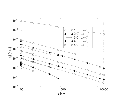
Figure 2: The absolute value of the oscillator strength $|f_{fi}|$ of the circular polarized transitions $\nu^{1}0^{+}\rightarrow\mu^{1}(-1)^{+}$ as a function of the field strength $\gamma$. On the left hand side from top to bottom the following transitions are shown $(\mu,\nu)=$ $(1,1)$,$(1,2)$, $(2,2)$, $(2,1)$, $(1,3)$, $(1,4)$, $(3,1)$, $(1,5)$, $(4,1)$, $(3,2)$, $(2,3)$, $(5,1)$, $(3,4)$, $(4,2)$, $(2,4)$, $(4,3)$, $(2,5)$, $(5,2)$, $(5,3)$.

In Figs. 3 – 8 the oscillator strengths of linear and circular polarized transitions are shown as a function of their wavelengths for different field strengths addressing the symmetry subspaces $\nu^{1}0^{+}$, $\nu^{3}0^{+}$, $\nu^{1}(-1)^{-}$, $\nu^{3}(-1)^{-}$, $\nu^{1}(-2)^{+}$, and $\nu^{3}(-2)^{+}$ for $\nu=1,\ldots,5$. With the exception of Figs 7 and 8 the range of wavelength shown is $10^{3}$ Å – $10^{5}$ Å.

Figure 3: The oscillator strengths $|f_{fi}|$ of the linear and circular polarized transitions emanating from the singlet states with zero magnetic quantum number and positive $z$ parity, i.e. $n^{1}0^{+},n=1,\ldots,5$ with their wavelength given in Å for $\gamma=100,200,1000,2000,10000$ a.u. from bottom to top.

Let us first discuss the oscillator strengths emanating from the singlet states with zero magnetic quantum number and positive $z$ parity (Fig. 3). With increasing field strength the transition wavelengths of some transitions decrease, whereas it increases for others. E.g. at $\approx 3000$ Å a gap between two groups of oscillator strengths emerges and widens with increasing field strength. The reader should note, that the values of the oscillator strengths correspondingly decrease. Similar statements hold also for the spectrum of the triplet transitions shown in Fig. 4.

Figure 4: The oscillator strength $|f_{fi}|$ of the linear and circular polarized transitions emanating from the triplet states with zero magnetic quantum number and positive $z$ parity, i.e. $n^{3}0^{+},n=1,\ldots,5$ with their wavelength given in Å for $\gamma=100,200,1000,2000,10000$ a.u. from bottom to top.

Figure 5: Same as in Fig. 3 but transitions emanating from the singlet states with $n^{1}(-1)^{-},n=1,\ldots,5$ for $\gamma=100,200,500,1000,2000$ a.u. from bottom to top.

The transition spectrum emanating from the states with magnetic quantum number $-1$ and negative $z$ parity shows a completely different pattern (see Figs. 5 and 6). The spectra are only reported up to $\gamma=2000$, since above this field strength there are no transitions between bound states including states of the ${}^{2S+1}(-1)^{-}$ symmetry. It can be observed that at $\gamma=100$ there are several very dominant transitions between $10^{3}$ Å and $10^{5}$ Å (up to 6 atomic units). The largest of these disappear with increasing field strength and at $\gamma=2000$ for ${}^{1}(-1)^{-}$, and $\gamma=1000$ for ${}^{3}(-1)^{-}$ respectively, only one transitions with an oscillator strengths of the order of one remains.

Figure 6: Same as in Fig. 5 but transitions emanating from the triplet states with magnetic quantum number $-1$ and negative $z$ parity for $\gamma=100,200,500,1000,2000$ a.u. from bottom to top.

Figure 7: Same as in Fig. 3 but transitions emanating from the singlet states with magnetic quantum number $-2$ and positive $z$ parity, i.e. $n^{1}(-2)^{+},n=1,\ldots,5$ with their wavelength given in Å for $\gamma=100,200,1000,2000,10000$ a.u. from bottom to top. Note the different length scales on the oscillator strength axis, for different field strengths.

In Figs. 7 and 8, the spectra for transitions emanating from the ${}^{2S+1}(-2)^{+}$ symmetry subspaces, are presented. For $\gamma=100,200$ a.u. the oscillator strength increase (with a few exceptions) monotonically as a function of the wavelength. For wavelengths of the order of $10^{3}$ Å, we find only oscillator strengths much smaller than 1, whereas for wavelengths in the interval $10^{4}-10^{5}$ Å the corresponding quantities are in the range $3-5$. At $\gamma=10000$, only one transition of the order of $0.002$ atomic units for a wavelength of approximately $10^{2}$ Å remains.

Figure 8: Same as in Fig. 7, but for transitions of corresponding triplet states, i.e. $n^{3}(-2)^{+},n=1,\ldots,5$ for $\gamma=100,200,1000,2000,10000$ atomic units from bottom to top. Note the different length scales on the oscillator strength axis, for different field strengths.

IV Brief conclusions

We have applied a full configuration interaction method to the helium atom in the superstrong field regime between $100$–$10\ 000$ atomic units. The effects of the finite nuclear mass have been taken into account. In this work we have presented results on the oscillator strengths between bound states. The operators, describing the dominating electric dipole transitions in the magnetic field in first order perturbation theory have been derived from first principles. It has been shown how the spectrum changes for different symmetries with increasing field strength. Finite nuclear mass effects decrease the number of bound state transitions in the superstrong field regime, since many states enter the continuum beyond a certain critical field strength. The influence of the finite nuclear mass on the oscillator strength has been analyzed.

For linear polarized transitions that do not involve tightly bound states the corresponding oscillator strengths are approximately field-independent and, compared to the results for infinite nuclear mass scaled by a factor involving the reduced mass. For linear polarized transitions involving tightly bound states the oscillator strengths obey a power law decay $f_{fi}(\gamma)\approx C\gamma^{-\lambda}$. A similar statement holds for the circular polarized transitions. Particular linear and circular polarized transitions do not belong to these two cases: they show a different strongly nonlinear dependence on the field strength.

Our results could be of relevance to the interpretation of spectra of neutron stars. For the future an investigation of the continuum would be very promising, particular since the discrete spectrum becomes very sparse in a superstrong field. The inclusion of motional electric fields into our study would also be very desirable. The latter requires however a major theoretical effort.

V Acknowledgments

The Deutsche Forschungsgemeinschaft is gratefully acknowledged for financial support. Discussions with S. Jordan, D. Wickramasinghe and J. Liebert are gratefully acknowledged.

References

- Friedrich and Wintgen (1989) H. Friedrich and D. Wintgen, Phys. Rep. 183, 37 (1989).
- Ruder et al. (1994) H. Ruder, G. Wunner, H. Herold, and F. Geyer, Atoms in strong magnetic fields (Springer Verlag, Berlin, 1994).
- Schmelcher and Schweizer (1998) P. Schmelcher and W. Schweizer, eds., Atoms and Molecules in Strong External Fields (Plenum Press, New York, 1998).
- Angel (1978) J. Angel, Ann. Rev. Astron. Astrophys. 16, 487 (1978).
- Pavlov et al. (1995) G. G. Pavlov, Y. A. Shibanov, V. E. Zavlin, and R. D. Meyer, in Proc. NATO ASI C 450, edited by M. A. Alpar, U. Kiziloǧlu, and J. van Paradijs (Kluwer, Dordrecht, 1995), pp. 71–90.
- Wickramasinghe and Ferrario (2000) D. T. Wickramasinghe and L. Ferrario, Pub. Astron. Soc. Pac. 112, 873 (2000).
- Angel et al. (1985) J. Angel, J. Liebert, and H. S. Stockmann, Astrophys. J. 292, 260 (1985).
- Greenstein et al. (1985) J. L. Greenstein, R. Henry, and R. F. O‘Connel, Astrophys. J. 289, L25 (1985).
- Wunner et al. (1985) G. Wunner, W. Rösner, H. Herold, and H. Ruder, Astron. Astrophys. 149, 102 (1985).
- Wickramasinghe and Ferrario (1988) D. T. Wickramasinghe and L. Ferrario, Astrophys. J. 327, 222 (1988).
- Kravchenko et al. (1996) Y. P. Kravchenko, M. A. Liberman, and B. Johansson, Phys. Rev. A 54, 287 (1996).
- Mueller et al. (1975) R. O. Mueller, A. Rau, and L. Spruch, Phys. Rev. A 11, 789 (1975).
- Virtamo (1976) J. Virtamo, J. Phys. B 9, 751 (1976).
- Pröschl et al. (1982) P. Pröschl, W. Rösner, G. Wunner, and H. Herold, J. Phys. B 15, 1959 (1982).
- Vincke and Baye (1989) M. Vincke and D. Baye, J. Phys. B 22, 2089 (1989).
- Braun et al. (1993) M. Braun, W. Schweizer, and H. Herold, Phys. Rev. A 48, 1916 (1993).
- Thurner et al. (1993) G. Thurner, H. Körbel, M. Braun, H. Herold, H. Ruder, and G. Wunner, J. Phys. B 26, 4719 (1993).
- Ivanov (1994) M. V. Ivanov, J. Phys. B 27, 4513 (1994).
- Braun et al. (1998) M. Braun, W. Schweizer, and H. Elster, Phys. Rev. A 57, 3739 (1998).
- Heyl and Hernquist (1998) J. S. Heyl and L. Hernquist, Phys. Rev. A 58, 3567 (1998).
- Becken et al. (1999) W. Becken, P. Schmelcher, and F. Diakonos, J. Phys. B 32, 1557 (1999).
- Becken and Schmelcher (2000) W. Becken and P. Schmelcher, J. Phys. B 33, 545 (2000).
- Becken and Schmelcher (2001) W. Becken and P. Schmelcher, Phys. Rev. A 63, 053412 (2001).
- Becken and Schmelcher (2002) W. Becken and P. Schmelcher, Phys. Rev. A 65, 033416 (2002).
- Green and Liebert (1980) R. F. Green and J. Liebert, Publ. Astr. Soc. Pac. 93, 105 (1980).
- Schmidt et al. (1990) G. D. Schmidt, W. B. Latter, and C. B. Foltz, Astrophys. J. 350, 768 (1990).
- Schmidt et al. (1996) G. D. Schmidt, R. G. Allen, P. S. Smith, and J. Liebert, Astrophys. J. 463, 320 (1996).
- Jordan et al. (1998) S. Jordan, P. Schmelcher, W. Becken, and W. Schweizer, Astron. Astrophys. Lett. 336, L33 (1998).
- Jordan et al. (2001) S. Jordan, P. Schmelcher, and W. Becken, Astron. Astrophys. 376, 614 (2001).
- Jones et al. (1999) M. D. Jones, G. Ortiz, and D. M. Ceperley, Phys. Rev. A 59, 2875 (1999).
- Al-Hujaj and Schmelcher (2003) O.-A. Al-Hujaj and P. Schmelcher, Phys. Rev. A 67, 023403 (2003).
- W. E. Lamb (1952) J. W. E. Lamb, Phys. Rev. 85, 259 (1952).
- Avron et al. (1978) J. E. Avron, I. W. Herbst, and B. Simon, Ann. Phys. 114, 431 (1978).
- Johnson et al. (1983) B. R. Johnson, J. O. Hirschfelder, and K. H. Yang, Rev. Mod. Phys. 55, 109 (1983).
- Schmelcher et al. (1994) P. Schmelcher, L. S. Cederbaum, and U. Kappes, in Conceptual Trends in Quantum Chemistry, edited by E. S. Kryachko and J. L. Calais (Kluwer, Dordrecht, 1994), pp. 1–51.
- Becken (2000) W. Becken, Ph.D. thesis, Universität Heidelberg (2000).
- Schmelcher and Cederbaum (1988) P. Schmelcher and L. S. Cederbaum, Phys. Rev. A 37, 672 (1988).
- Kappes and Schmelcher (1996) U. Kappes and P. Schmelcher, Phys. Rev. A 54, 1313 (1996), 53, 3869 (1996); 51, 4542 (1995).
- Detmer et al. (1997) T. Detmer, P. Schmelcher, F. K. Diakonos, and L. S. Cederbaum, Phys. Rev. A 56, 1825 (1997).
- Detmer et al. (1998) T. Detmer, P. Schmelcher, and L. S. Cederbaum, Phys. Rev. A 57, 1767 (1998); 61, 043411 (2000); 64, 023410 (2001); J. Chem. Phys., 109 (1998); J. Phys. B 28 (1995).
- Al-Hujaj and Schmelcher (2000) O.-A. Al-Hujaj and P. Schmelcher, Phys. Rev. A 61, 063413 (2000).