Spinning eggs—which end will rise?

Abstract

We examine the spinning behavior of egg-shaped axisymmetric bodies whose cross sections are described by several oval curves similar to real eggs with thin and fat ends. We use the gyroscopic balance condition of Moffatt and Shimomura and analyze the slip velocity of the bodies at the point of contact as a function of $\theta$, the angle between the axis of symmetry and the vertical axis, and find the existence of the critical angle $\theta_{c}$. When the bodies are spun with an initial angle $\theta_{\rm initial}>\theta_{c}$, $\theta$ will increase to $\pi$, implying that the body will spin at the thin end. Alternatively, if $\theta_{\rm initial}<\theta_{c}$, then $\theta$ will decrease. For some oval curves, $\theta$ will reduce to 0 and the corresponding bodies will spin at the fat end. For other oval curves, a fixed point at $\theta_{f}$ is predicted, where $0<\theta_{f}<\theta_{c}$. Then the bodies will spin not at the fat end, but at a new stable point with $\theta_{f}$. The empirical fact that eggs more often spin at the fat than at the thin end is explained.

I Introduction

Spinning objects have historically been interesting subjects to study. The spin reversal of the rattlebackGH (also called a celt or wobblestone) and the behavior of the tippe topGN are typical examples. Recently, the riddle of spinning eggs was resolved by Moffatt and Shimomura.MS When a hard-boiled egg is spun sufficiently rapidly on a table with its axis of symmetry horizontal, the axis will rise from the horizontal to the vertical. They discovered that if an axisymmetric body is spun sufficiently rapidly, a gyroscopic balance condition holds. Given this condition a constant of the motion exists for the spinning motion of an axisymmetric body. The constant, which is known as the Jellett constant,Jellett has been found previously for symmetric tops such as the tippe top. Using these facts, they derived a first-order differential equation for $\theta$, the angle between the axis of symmetry and the vertical axis. For a uniform spheroid as an example they showed that the axis of symmetry indeed rises from the horizontal to the vertical.

The shape of an egg looks like a spheroid, but is not exactly so. It has thin and fat ends. Which end of the spinning egg will rise? Empirically, we know that either end can rise. But we more often see eggs spinning at the fat end with the thin end up rather than the other way round. In this paper we investigate the spinning behavior of egg-shaped axisymmetric bodies whose cross sections are described by several oval curves. We use the gyroscopic balance condition and analyze the slip velocity of the body at the point of contact as a function of $\theta$ and find the existence of the critical angle $\theta_{c}$ for each model curve. When the bodies are spun with the initial angle $\theta_{\rm initial}>\theta_{c}$, $\theta$ will increase to $\pi$, which means that the body will spin at the thin end. Alternatively, if $\theta_{\rm initial}<\theta_{c}$, then $\theta$ will decrease. For some oval curves, $\theta$ will decrease to 0 and the corresponding bodies will shift to the stable spinning state at the fat end. For other oval curves, a fixed point at $\theta_{f}$ is predicted, where $0<\theta_{f}<\theta_{c}$. In this case the bodies will spin not at the fat end but at a new stable point with $\theta_{f}$. We also explain why we observe more eggs spinning at the fat end than at the thin end.

The paper is organized as follows: To explain our notation and the geometry, we review the work of Ref. MS, on spinning eggs in Sec. II. Then in Sec. III we introduce several models of oval curves that we will study. In Sec. IV we analyze the spinning behavior of axisymmetric bodies whose cross sections are described by these oval curves. The final section is devoted to a summary and discussion.

II Spinning egg

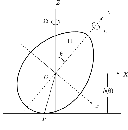
Figure 1: An axisymmetric body with center of mass $O$ on a horizontal table with point of contact $P$. Its axis of symmetry, $O\!z$, and the vertical axis, $O\!Z$, define a plane $\Pi$, which precesses about $O\!Z$ with angular velocity $\boldsymbol{\Omega}(t)=(0,0,\Omega)$. $O\!X\!Y\!Z$ is a rotating frame of reference with $O\!X$ horizontal in the plane $\Pi$. The height of $O$ above the table is $h(\theta)$ (from Ref. 3).

We follow the geometry and notation of Ref. MS, in their analysis of spinning eggs as much as possible. As is shown in Fig. 1, an axisymmetric body spins on a horizontal table with point of contact $P$. We will work in a rotating frame of reference $O\!X\!Y\!Z$, where the center of mass is at the origin, $O$. The symmetry axis of the body, $O\!z$, and the vertical axis, $O\!Z$, define a plane $\Pi$, which precesses about $O\!Z$ with angular velocity $\boldsymbol{\Omega}(t)=(0,0,\Omega)$. We choose the horizontal axis $O\!X$ in the plane $\Pi$ and thus $O\!Y$ is vertical to $\Pi$ and inward. The angle of interest is $\theta(t)$, the angle between $O\!Z$ and $O\!z$.

In a rotating frame of reference $O\!xyz$, where $O\!x$ is in the plane $\Pi$ and perpendicular to the symmetry axis $O\!z$ and where $O\!y$ coincides with $O\!Y$, the body spins about $O\!z$ with the rate $\dot{\psi}$. Since, in the frame $O\!xyz$, $\boldsymbol{\Omega}$ is expressed as $\boldsymbol{\Omega}=-\Omega\sin\theta\hat{x}+\Omega\cos\theta\hat{z}$, the angular velocity of the body, $\boldsymbol{\omega}$, is given by $\boldsymbol{\omega}=-\Omega\sin\theta\hat{x}+\dot{\theta}\hat{y}+n\hat{z}$. Here ${\hat{x}}$, ${\hat{y}}$, and ${\hat{z}}$ are unit vectors along $O\!x$, $O\!y$, and $O\!z$, respectively, $n(t)$ is given by $n=\Omega\cos\theta+\dot{\psi}$, and the dot represents differentiation with respect to time. The $O\!x$ and $O\!y$ axes are not body-fixed axes but they are principal axes, so that the angular momentum, $\boldsymbol{L}$, is expressed by $\boldsymbol{L}=-A\Omega\sin\theta\hat{x}+A\dot{\theta}\hat{y}+Cn\hat{z}$, where $(A,A,C)$ are the principal moments of inertia at $O$.

The coordinate system $O\!X\!Y\!Z$ is obtained from the frame $O\!xyz$ by rotating the latter about the $O\!y$ ($O\!Y$) axis through the angle $\theta$. Hence, in the rotating frame $O\!X\!Y\!Z$, $\boldsymbol{\omega}$, and $\boldsymbol{L}$ have components

$$\boldsymbol{\omega} = \big{(}(n-\Omega\cos\theta)\sin\theta,\dot{\theta},\Omega\sin^{2}\theta+n\cos\theta\big{)},$$ (1)

$$\boldsymbol{L} = \big{(}(Cn-A\Omega\cos\theta)\sin\theta,A\dot{\theta},A\Omega\sin^{2}\theta+Cn\cos\theta\big{)},$$ (2)

respectively. The evolution of $\boldsymbol{L}$ is governed by Euler’s equation,

$$\frac{\partial\boldsymbol{L}}{\partial t}+\boldsymbol{\Omega}\times\boldsymbol{L}=\boldsymbol{X}\!_{P}\times(\boldsymbol{R}+\boldsymbol{F}),$$ (3)

where $\boldsymbol{X}\!_{P}$ is the position vector of the contact point $P$ from $O$, $\boldsymbol{R}$ is the normal reaction at $P$, $\boldsymbol{R}=(0,0,R)$, with $R$ being of order $M\!g$, the weight, and $\boldsymbol{F}$ is the frictional force at $P$. Because the point $P$ lies in the plane $\Pi$, $\boldsymbol{X}\!_{P}$ has components $(X\!_{P},0,Z_{p})$, which are given by

$$Z_{P} = -h(\theta)$$ (4a)

$$X\!_{P} = \frac{dh}{d\theta},$$ (4b)

where $h(\theta)$ is the height of $O$ above the table. We will see in Sec. IV that $h(\theta)$ is determined as a function of $\theta$, once the geometry and density distribution of the body are known.

When the frictional force is weak and $\dot{\theta}$ is correspondingly small, the slip velocity of the point $P$ is, to leading order in $\dot{\theta}$, expressed as $\boldsymbol{U}\!_{P}=(0,V_{P},0)$, where

$$V_{P}=(\Omega\sin^{2}\theta+n\cos\theta)\frac{dh}{d\theta}+(n-\Omega\cos\theta)h(\theta)\sin\theta.$$ (5)

Hence, the frictional force, $\boldsymbol{F}$, is to leading order, $\boldsymbol{F}=(0,F,0)$, where $F$ is a function of $V_{P}$ given by the law of dynamic friction between the two surfaces in contact. We assume later Coulomb friction for $F$.

The $Y$-component of Eq. (3) is expressed by

$$A{\ddot{\theta}}+(Cn-A\Omega\cos\theta)\Omega\sin\theta=-RX\!_{P}~{}.$$ (6)

Since the secular change of $\theta$ with which we are concerned is slow and thus $|\ddot{\theta}|\ll\Omega^{2}$, the first term of Eq. (6) can be neglected. Furthermore, in a situation where $\Omega^{2}$ is sufficiently large so that the terms involving $\Omega$ in Eq. (6) dominate the term $-RX\!_{P}$, Eq. (6) is reduced, at leading order, to $(Cn-A\Omega\cos\theta)\Omega\sin\theta=0$. Then, for $\sin\theta\not=0$, we arrive at a condition

$$Cn=A\Omega\cos\theta,$$ (7)

which was recently discovered by Moffatt and ShimomuraMS and was called by them as the gyroscopic balance condition. Under this condition, the Jellett constantJellett also exists for a general axisymmetric body. With Eq. (7), the angular momentum simplifies to $\boldsymbol{L}=(0,A{\dot{\theta}},A\Omega)$, and the $X$- and $Z$-components of Eq. (3) reduce, respectively, to

$$A\Omega\dot{\theta}=FZ\!_{P},$$ (8a)

$$A\dot{\Omega}=FX\!_{P}.$$ (8b)

Equation (8), together with Eq. (4), leads to

$$-\boldsymbol{L}\cdot\boldsymbol{X}\!_{P}=A\Omega h=J=\mbox{constant},$$ (9)

where the Jellett constant $J$ is determined by the initial conditions. From Eqs. (4), (9), and (8a), we obtain a first-order differential equation for $\theta$,

$$J\dot{\theta}=-Fh^{2}(\theta).$$ (10)

If we assume Coulomb friction, $F$ is given by

$$F=-\mu Mg\frac{V_{P}}{|V_{P}|},$$ (11)

and $V_{P}$ in Eq. (5), given the gyroscopic balance condition (7), is expressed as a function of $\theta$ as:

$$V_{P}=\frac{J}{Ah(\theta)}\bigg{[}\Big{(}\sin^{2}\theta+\frac{A}{C}\cos^{2}\theta\Big{)}\frac{dh}{d\theta}+\sin\theta\cos\theta\Big{(}\frac{A}{C}-1\Big{)}h(\theta)\bigg{]}.$$ (12)

Hence, if we know $h(\theta)$ from geometrical considerations , we may solve Eq. (10) and determine the time-dependence of $\theta$. Moffatt and ShimomuraMS considered a uniform spheroid as an example and showed that $\theta$ decreases from $\pi/2$ to 0 for the prolate spheroid while $\theta$ increases from 0 to $\pi/2$ for the oblate one.

However, the shape of an egg is not a spheroid and has thin and fat ends. Which end of the spinning egg will rise? Empirically, we know that either end may rise and that the body spins with its axis of symmetry vertical. Which end the spinning egg chooses might seem to depend on the inclination of the initial axis of symmetry, that is, the initial value of $\theta$. In the following we examine several models of oval curves and determine the relation between the initial value of $\theta$ and the final spinning position of the egg-shaped body.

III Models of oval curve

The shape of a three-dimensional egg can be reconstructed by rotating its two-dimensional cross section around the axis of symmetry. The cross section of an egg looks similar to an ellipse, but is not quite. It is sharper at one end than at the other. We will examine several model curves that have been proposed for the cross-section of a real egg.

Let us consider an axisymmetric body whose cross-section is described by

$$x^{2}=g(z),$$ (13)

with $g(z)>0$ for $z_{\min}<z<z_{\max}$ and $g(z_{\min})=g(z_{\max})=0$, where we choose the $z$ axis as the symmetry axis. If the body has uniform density, then the volume and the $z$ component of center of mass are given, respectively, by

$$V = \pi\!\int^{z_{\max}}_{z_{\min}}g(z)\,dz,$$ (14a)

$$z_{g} = \frac{\pi}{V}\!\int^{z_{\max}}_{z_{\min}}zg(z)\,dz.$$ (14b)

The principal moments of inertia at center of mass are expressed by

$$A = M\frac{\pi}{V}\!\int^{z_{\max}}_{z_{\min}}\bigg{[}\frac{1}{4}[g(z)]^{2}+g(z)(z-z_{g})^{2}\bigg{]}dz,$$ (15a)

$$C = \frac{M}{2}\frac{\pi}{V}\!\int^{z_{\max}}_{z_{\min}}[g(z)]^{2}\,dz.$$ (15b)

Of course, the density of a real egg is not uniform. But if the density distribution is given by $\rho(r,z)$ as a function of $r$ and $z$, where $r$ is the distance from the symmetry axis, and the cross-section is still described by Eq. (13), we can calculate $z_{g}$, $A$, and $C$.

The following are the oval curves that we will examine.

1. Cartesian oval. The curve, given by $\sqrt{z^{2}+x^{2}}+m\sqrt{(z+a)^{2}+x^{2}}=c$, consists of two ovals. For definiteness we set $m=2$. The inside oval is expressed by $x^{2}=g(z)$ with

   $$g(z)=-z^{2}-\frac{8}{3}az+\frac{a^{2}}{9}(5\kappa^{2}-12)-\frac{4}{9}\kappa a^{2}\sqrt{\kappa^{2}-3-\frac{6z}{a}},$$ (16)

   with $\kappa=c/a$. For $\kappa=9/4$, we find that $g(z)$ is defined for the interval $-\frac{17}{12}a\leq z\leq\frac{1}{12}a$, $z_{g}=-0.710a$, and $A/C=1.26$ (see Fig. 2).

2. Cassini oval. This quartic curve is expressed by $[(z+a)^{2}+x^{2}][(z-a)^{2}+x^{2}]=b^{4}$ with $a,b>0$. If $a>b$, the curve consists of two loops, both of which look like the cross-section of a real egg with thin and fat ends. We choose the one that is expressed by $x^{2}=g(z)$ with

   $$g(z)=-(z^{2}+a^{2})+a\sqrt{4z^{2}+\lambda^{4}a^{2}},$$ (17)

   where $\lambda=\frac{b}{a}<1$ for $-a\sqrt{1+\lambda^{2}}\leq z\leq-a\sqrt{1-\lambda^{2}}$, so that the thin end points to the positive $z$ axis (see Fig. 3). For $\lambda=0.98$, we find $z_{\min}=-1.40a$, $z_{\max}=-0.199a$, $z_{g}=-0.840a$, and $A/C=1.25$.

3. Cassini oval with an air chamber. A real egg has an air chamber near the fat end. We take into account the existence of an air chamber by using the Cassini oval (17) and taking $z_{\min}=-\alpha a$, with $\sqrt{1-\lambda^{2}}<\alpha<\sqrt{1+\lambda^{2}}$ for the evaluation of $V$, $z_{g}$, $A$, and $C$. This condition means that an empty space exists for $-\sqrt{1+\lambda^{2}}a\leq z\leq-\alpha a$ (see Fig. 4). For $\lambda=0.98$ and $\alpha=1.2$, we obtain $z_{g}=-0.798a$ and $A/C=1.07$. The position of the center of mass $z_{g}$ is closer to the thin end and the ratio $A/C$ is smaller compared to the curve without an air chamber.

4. Wassenaar egg curve. A rather simple equation for an oval curve was proposed recently by WassenaarWassenaar and is given by

   $$x^{2}=g(z)=2a\big{[}-2z-\xi a+\sqrt{4a^{2}+4\xi az+\xi^{2}a^{2}}\big{]},$$ (18)

   for $5<\xi<6$ and $-a\leq z\leq a$. For $\xi=5.6$ we find $z_{g}=-0.0714a$ and $A/C=1.21$ (see Fig. 5).

5. Lemniscate of Bernoulli. The lemniscate of Bernoulli is not a candidate for oval curves and actually looks like the infinity symbol. We study it because its final spinning position might be interesting. The curve is expressed by $[(z+a)^{2}+x^{2}][(z-a)^{2}+x^{2}]=a^{4}$. We study the half of the curve that is given by

   $$x^{2}=g(z)=-(z^{2}+a^{2})+a\sqrt{4z^{2}+a^{2}},$$ (19)

   with $-\sqrt{2}a\leq z\leq 0$. The lemniscate is a special case of a Cassini oval and is obtained by setting $a=b$ in Eq. (17). For the lemniscate, we obtain $z_{g}=-0.813a$ and $A/C=1.34$ (see Fig. 6).

We plot in Fig. 7 the Cartesian and Cassini ovals and the Wassenaar egg curve, adjusting the parameter $a$ for each case so that they have the same length along the symmetry axis. We observe that the Cartesian and Cassini ovals almost overlap. Indeed the axisymmetric bodies whose cross sections are expressed by these oval curves have close values of $A/C$ (1.26 and 1.25 for the Cartesian and Cassini ovals, respectively). However, we will see in Sec. IV that these ovals predict different spinning behavior for the corresponding axisymmetric bodies.

IV Which end will rise?

We obtain from Eqs. (10) and (11)

$$\dot{\theta}=\frac{\tau}{|V_{P}|}{\widetilde{V}}_{P},$$ (20)

with

$${\widetilde{V}}_{P}=V_{P}\frac{A}{J}\quad{\rm and}\quad\tau=\frac{h^{2}\mu Mg}{A}.$$ (21)

Equation (20) implies that the change of $\theta$ is governed by the sign of ${\widetilde{V}}_{P}$. If ${\widetilde{V}}_{P}$ is positive (negative), $\theta$ will increase (decrease) with time. Therefore a close examination of the behavior of ${\widetilde{V}}_{P}$ as a function of $\theta$ will be important. Moffatt and ShimomuraMS showed that for a uniform prolate spheroid, ${\widetilde{V}}_{P}$ has the form ${\widetilde{V}}_{P}\propto\sin 2\theta$ with a negative proportionality constant. Thus if the body is spun (sufficiently rapidly) on a table with the initial inclination angle $\theta_{\rm initial}<\pi/2$, then $\theta$ decreases to 0. On the other hand, if the body is spun with $\theta_{\rm initial}>\pi/2$, $\theta$ increases to $\pi$. Either end will rise, because both ends of the prolate spheroid look the same. The case of a real egg is different. We can easily distinguish between the thin and the fat end. We will now analyze the axisymmetric bodies whose cross-sections are expressed by the oval curves introduced in Sec. III.

We take a coordinate system in which the center of mass $O$ resides at the origin. In this coordinate system, the oval curves satisfy

$$x^{2}=f(z)=g(z+z_{g}),$$ (22)

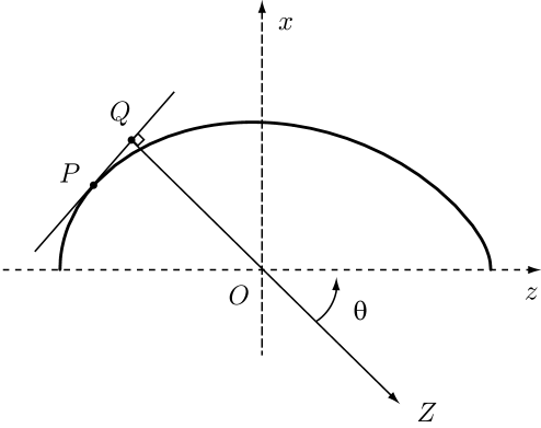
Figure 8: An oval curve $x=\sqrt{f(z)}$ that describes a part of the cross section of an axisymmetric body. The center of mass $O$ is at the origin. The line $OQ$ is perpendicular to the line tangent to the curve at the point $P(z,x=\sqrt{f(z)})$. The line $PQ$ is on a horizontal table and $P$ corresponds to the point of contact. The line $QO$ defines the vertical axis $OZ$, and the polar angle $\theta$ between $OZ$ and $Oz$ is given by $\tan\theta=1/\beta$, where $\beta$ is the slope of the line tangent to the curve at $P$. The length of $OQ$ is $h(\theta)$.

where $g(z)$ is introduced in Eq. (13) to describe the cross-section of an axisymmetric body whose center of mass is at $z=z_{g}$. We consider the point $P$($z,x=\!\sqrt{f(z)}$) on the curve (see Fig. 8). The slope $\beta$ of the line tangent to the curve at $P$ is given by

$$\beta\equiv\frac{dx}{dz}=\frac{f^{\prime}(z)}{2\sqrt{f(z)}}.$$ (23)

Draw a line from the origin which is perpendicular to the line tangent to the curve $x=\sqrt{f(z)}$ at $P$. Let the point of intersection be $Q$($z_{Q},x_{Q}$), whose coordinates are

$$z_{Q} = \frac{\beta}{\beta^{2}+1}(\beta z-\sqrt{f(z)}),$$ (24a)

$$x_{Q} = -\frac{1}{\beta}z_{Q}.$$ (24b)

Suppose that the line $PQ$ is in a horizontal plane of table and $P$ is the point of contact. Then the line $QO$ defines the vertical axis $OZ$. The polar angle, $\theta$, between $OZ$ and $Oz$ is determined by,

$$\tan\theta=\frac{1}{\beta}=\frac{2\sqrt{f(z)}}{f^{\prime}(z)},$$ (25)

which gives the relation between $\theta$ and $z$. The height, $h(\theta)$, of $O$ above the table is equal to the length of $OQ$, and we obtain

$$h(\theta)=\sqrt{z_{Q}^{2}+x_{Q}^{2}}=\frac{1}{\sqrt{\beta^{2}+1}}(\sqrt{f(z)}-\beta z),$$ (26)

because $(\sqrt{f(z)}-\beta z)>0$. The squared length of $PQ$ corresponds to $X\!_{P}^{2}$. We choose the sign of $X\!_{P}$ to be the same as that of $(z-z_{Q})$ and obtain

$$X\!_{P}=\frac{1}{\sqrt{\beta^{2}+1}}\Big{(}z+\beta\sqrt{f(z)}\Big{)}.$$ (27)

If we use Eqs. (25)–(27), we confirm Eq. (4b) and find that $V_{P}$ in Eq. (12) can be rewritten as a function $z$ as follows:

$$V_{P}=\frac{J}{A}\frac{\beta^{2}}{\beta^{2}+1}\bigg{[}\Big{(}\frac{1}{\beta^{2}}+\frac{A}{C}\Big{)}\frac{z+\beta\sqrt{f(z)}}{\sqrt{f(z)}-\beta z}+\frac{1}{\beta}\Big{(}\frac{A}{C}-1\Big{)}\bigg{]}.$$ (28)

From Eq. (25), $X_{P}$ and $V_{P}$ can be considered as functions of $\theta$. As an example, we plot in Fig. 9 the graph of $X_{P}$ versus $\theta$ for the case of the Cartesian oval in Eq. (16). In addition to $\theta=0$ and $\pi$, $X_{P}$ vanishes at an angle $\theta_{r}$, which is obtained by solving

$$z+\beta\sqrt{f(z)}=0.$$ (29)

When the body is placed at rest on a table, its inclination angle is $\theta_{r}$ and the height $h(\theta)$ of center of mass $O$ from the table is a minimum at $\theta_{r}$. We observe from Eqs. (5) or (12) that $V_{P}=0$ at $\theta=0$ and $\pi$, because $\sin\theta=0$ and $\frac{dh}{d\theta}(=X_{p})=0$ at these points. Moreover, $V_{P}$ vanishes at other angles, which are given by solving

$$\frac{A}{C}+\frac{z}{\beta\sqrt{f(z)}}=0.$$ (30)

When $A=C$, Eqs. (29) and (30) become equivalent, which means that $V_{P}$ and $X_{P}$ vanish at the same inclination angle.

We next examine the graph of ${\widetilde{V}}_{P}$ as a function of $\theta$ for the oval curves introduced in Sec. III.

(i) A Cartesian oval. Figure 10 shows that ${\widetilde{V}}_{P}$ crosses the line ${\widetilde{V}}_{P}=0$ at an angle $\theta_{c}$ and ${\widetilde{V}}_{P}>0$ for $\theta_{c}<\theta<\pi$ but is negative for $0<\theta<\theta_{c}$. So, the angle $\theta_{c}$ is a critical point. If the body is spun on a table with the initial angle $\theta_{\rm initial}>\theta_{c}$, then $\theta$ will increase to $\pi$, which means that the body will eventually spin at the thin end. For $\theta_{\rm initial}<\theta_{c}$, we will see that the body spins at the fat end. That is, depending on the initial value $\theta_{\rm initial}$, the body will spin at the thin or the fat end. Both ends are stable points. We have $A>C$ for Cartesian ovals, which leads to $\theta_{c}>\theta_{r}$. Numerically we obtain from Eqs. (30) and (29) that $\theta_{c}=1.86$ and $\theta_{r}=1.72$. Recall that $\theta_{r}$ is the inclination angle when the body is placed at rest. If we spin the body involuntarily, the initial angle $\theta_{\rm initial}$ tends to be near $\theta_{r}$. Because $0<\theta_{r}<\theta_{c}$, it is likely that the body is spun with $\theta_{\rm initial}$ between 0 and $\theta_{c}$, and thus it will shift to the stable spinning state at the fat end. Empirically, we more often observe eggs spinning at the fat end rather than at the thin end. The expected behavior of the axisymmetric body expressed by the Cartesian oval in Eq. (16) well explains the observed features of the spinning egg.

(ii) A Cassini oval. The second example of oval curves presents an interesting situation. We see from Fig. 11 that ${\widetilde{V}}_{P}$ crosses the line ${\widetilde{V}}_{P}=0$ at $\theta_{f}$ and $\theta_{c}$ ($\theta_{f}<\theta_{c}$), and that ${\widetilde{V}}_{P}$ is negative for $\theta_{f}<\theta<\theta_{c}$ and otherwise positive. Numerically we obtain $\theta_{f}=0.45$ and $\theta_{c}=1.92$ (and $\theta_{r}=1.77$). Thus the graph of ${\widetilde{V}}_{P}$ in Fig. 11 implies that for the Cassini oval (17) the thin end ($\theta=\pi$) is a stable point, but the fat end is not. When the body is spun with the initial value of $\theta$ anywhere between 0 and $\theta_{c}$, $\theta$ will approach the fixed point $\theta_{f}$. In other words, the body will spin not at the fat end, but at the point with the inclination angle $\theta_{f}$. It is interesting to note that the curves of the Cartesian (16) and Cassini (17) ovals almost overlap each other when they are adjusted to have the same length along the symmetry axis (see Fig. 7). But they predict different behaviors for ${\widetilde{V}}_{P}$ and thus different spinning behaviors for the corresponding axisymmetric bodies. Does a hard boiled egg show the behavior predicted by this Cassini oval? We are almost certain that we have never seen such a behavior.

(iii) A Cassini oval with an air chamber. Because an egg has an air chamber near the fat end, we study the case of a Cassini oval with an air chamber. The existence of an air chamber moves the position of center of mass $z_{g}$ toward the thin end, from $z_{g}=-0.840a$ to $z_{g}=-0.798a$, and reduces the ratio $A/C$ from 1.25 to 1.07. Consequently, the fixed point at $\theta_{f}$, which is present for Eq. (17), disappears. The graph of ${\widetilde{V}}_{P}$ in Fig. 12 shows that it crosses the line ${\widetilde{V}}_{P}=0$ only once at $\theta_{c}=1.97$. The inclination angle at rest becomes $\theta_{r}=1.93$, which is very close to the value of $\theta_{c}$ because $A/C\approx 1$. The axisymmetric body described by a Cassini oval with an air chamber also reproduces the features of the spinning egg.

(iv) Wassenaar egg curve. Figure 13 shows that this curve has a fixed point at $\theta_{f}=0.93$. When $\theta_{\rm initial}$ is between 0 and $\theta_{c}=1.85$, $\theta$ will move to $\theta_{f}$, another stable point in addition to the one at the thin end ($\theta=\pi$). In addition, the graph of $X_{P}$ for this oval curve vanishes at two other points. One is at $\theta_{r}=1.78$, a position at rest, and one at $\theta=0.58$, an unstable point.

(v) Lemniscate of Bernoulli. For the lemniscate of Bernoulli, we find $\lim_{z\rightarrow z_{\max}}(1/\beta)=-1$, so that Eq. (25) tells us that the allowed region of $\theta$ is between 0 and $3\pi/4$. Figure 14 shows that ${\widetilde{V}}_{P}$ vanishes at the fat end ($\theta=0$), at the fixed point ($\theta_{f}=0.74$), and at the critical point ($\theta_{c}=1.96$). The position of the body at rest is at $\theta_{r}=1.81$, and its spinning state has two stable points at $\theta=\theta_{f}$ and $3\pi/4$.

V Summary and Discussion

We have examined the spinning behavior of axisymmetric bodies whose cross sections are described by several model curves, including a Cartesian oval, Cassini ovals with and without an air chamber, and the Wassenaar egg curve. These results together with the lemniscate of Bernoulli are summarized in Table 1. For each oval curve we used the gyroscopic balance condition (7) and found the predicted slip velocity $V_{P}$ of the contact point as a function of the inclination angle $\theta$ and the existence of the critical angle $\theta_{c}$. When the body is spun on a table with the initial angle $\theta_{\rm initial}>\theta_{c}$, $\theta$ will increase to $\pi$, which means that the body will spin at the thin end. If $\theta_{\rm initial}<\theta_{c}$, then $\theta$ will decrease. For the Cartesian oval and Cassini oval with an air chamber, $\theta$ will reduce to 0 and the corresponding bodies will spin at the fat end. Moreover, when the bodies are spun without intention, we expect to see their spinning states at the fat end more often than at the thin end because the inclination angle $\theta_{r}$ at rest is smaller than $\theta_{c}$. This behavior is consistent with the features of a spinning egg.

On the other hand, the Cassini oval and Wassenaar egg curves predict the existence of the fixed point at $\theta_{f}$, where $0<\theta_{f}<\theta_{c}$. Then the fat end ($\theta=0$) is no longer a stable point. If the corresponding bodies are spun with $\theta_{\rm initial}<\theta_{c}$, $\theta$ moves to $\theta_{f}$ and not to 0, and the bodies will spin at a new stable point at $\theta_{f}$. The lemniscate of Bernoulli is not an oval curve, but the body described by this curve also has a fixed point.

It would be very interesting to make axisymmetric bodies whose cross sections are described by the Cassini oval (17), Wassenaar egg curve (18) and the lemniscate of Bernoulli (19) and determine if those bodies will spin at a new stable point that is different from the fat end.

The inclusion of an air chamber at the fat end tends to diminish the appearance of the fixed point at $\theta_{f}$. The case of a Cassini oval is an example. For the Wassenaar egg curve, we need a rather large air chamber; an empty space for $-a\leq z\leq-0.5a$ in Eq. (18) is necessary for the disappearance of $\theta_{f}$. The fixed point of the lemniscate vanishes if we take $z_{\min}=-1.33a$ for Eq. (19). Moreover, the inclusion of an air chamber at the fat end moves the position of the center of mass $z_{g}$ toward the thin end and makes the ratio $A/C$ smaller. Consequently, the values of the critical angle $\theta_{c}$ and the inclination angle at rest $\theta_{r}$ move toward $\pi$.

We have assumed Coulomb’s law for the friction $F$ (see Eq. (11)). If we instead assume a viscous friction law,

$$F=-{\tilde{\mu}}MgV_{P},$$ (31)

all our conclusions remain unchanged, in particular, the positions of the critical points and fixed points. Only the transition time from the unstable to the stable state will be modified. As an example, the transition time from the angle $\theta_{c}$ to $\pi$ is numerically calculated to be $t(\theta_{c}\rightarrow\pi)=(J/\mu Mga^{2})\chi$ with a numerical factor $\chi\sim{\cal O}(1)$ for Coulomb friction, and $t(\theta_{c}\rightarrow\pi)=(1/{\tilde{\mu}}g)\chi$ with $\chi\sim{\cal O}(10)$ for viscous friction .

Oval curves	Critical	The angle	Fixed point	Spin at	Spin at
	angle $\theta_{c}$	at rest $\theta_{r}$	angle $\theta_{f}$	the fat end	the thin end
Cartesian oval [Eq. (16)]	1.86	1.72	Not exist	Yes	Yes
Cassini oval [Eq. (17)]	1.92	1.77	0.45	No	Yes
Cassini oval [Eq. (17)] with	1.97	1.93	none	Yes	Yes
an air chamber ($z_{\min}=-1.2a$)
Wassenaar egg curve [Eq. (18)]	1.85	1.78	0.93	No	Yes
Lemniscate [Eq. (19)]	1.96	1.81	0.74	No	No

Table 1: Predicted values of the critical angle $\theta_{c}$, the inclination angle at rest $\theta_{r}$, and the fixed point angle $\theta_{f}$ for the axisymmetric bodies whose cross sections are described by the various oral curves. Also tabulated are the predicted possibilities of those axisymmetric bodies spinning at the fat and/or the thin end.

Figures

Figure 2: A Cartesian oval in units of the arbitrary length $a$.

Figure 3: A Cassini oval in units of $a$.

Figure 4: A Cassini oval with air chamber in units of $a$.

Figure 5: Wassenaar egg curve in units of $a$.

Figure 6: The lemniscate in units of $a$.

Figure 7: The Cartesian oval (a solid curve), Cassini oval (short-dashed curve), and a proposed egg curve (dashed curve) adjusted to have the same length along the symmetry axis.

Figure 9: $X_{P}$ as a function of $\theta$ for a Cartesian oval.

Figure 10: ${\widetilde{V}}_{P}$ as a function of $\theta$ for a Cartesian oval.

Figure 11: ${\widetilde{V}}_{P}$ as a function of $\theta$ for a Cassini oval.

Figure 12: ${\widetilde{V}}_{P}$ as a function of $\theta$ for a Cassini oval with an air chamber.

Figure 13: ${\widetilde{V}}_{P}$ as a function of $\theta$ for Wassenaar egg curve.

Figure 14: ${\widetilde{V}}_{P}$ as a function of $\theta$ for the lemniscate.