Note on the typhoon eye trajectory
Olga Rozanova
Department of Differential Equations, Mathematics and Mechanics Faculty
Moscow State University
GSP-2 Vorobiovy Gory 119992 Moscow Russia
E-mail: rozanova@mech.math.msu.su
Abstract
We consider a model of typhoon based on the three-dimensional baroclinic compressible equations of atmosphere dynamics averaged over hight and describe a qualitative behavior of the vortex and possible trajectories of the typhoon eye.
2000 Mathematics Subject Classification:35Q30; 85A10; 76N15; 35L65.
1 Preliminaries
The typhoon (or tropical hurricane) is an intense vortex of middle scale in the atmosphere having radius in several hundred kilometers. It is a stable structure, existing sometimes within more then two weeks. The typhoon trajectory can be very complicated, it can suddenly change the direction, make loops, the motion stops sometimes for several days. The speed of wind in the vortex region may amount to The huge experimental information, including the archive of hurricanes paths can be found on the following sites: [1]. The physical processes inside of typhoon are complex [2],[3], for a sufficient description of this phenomenon they use nonlinear systems of PDE in three spatial dimensions, that can be solved only numerically.
However, there are attempts to explain qualitative properties of of typhoon’s behavior by means of simplified hydrodynamical models. Note before all the outstanding paper by N.E.Kochin of 1922 [4], where the cyclone model based on the conditions of dynamic possibility in the sense of A.A.Fridman was considered. The theory predicts that the trajectory may have loops and the points of return. Earlier Rayleigh [5], Show [6], Fridman[7] studied the trajectories of atmospheric vortices.
There exists a trend where methods of the solid state mechanics are applied for a study of peculiarities of the tropical cyclones trajectory. Here the tropical cyclone is modelled as a rigid rotating cylinder (or a washer) in a flow of viscous fluid and an evaluation of different forces acting to the cylinder are made. In [8] the Coriolis force acting to the vertical component of velocity inside of the typhoon is estimated, in [9, 10, 11] the lifting (the Zhukovskii force), the friction against a bedding surface and the drag force are considered, in [12, 13] all forces mentioned are taken into account. However, under this approach the problem is a determination of the main flow (generally speaking, it is assumed as given). If the cyclone trajectory deviates from the trajectory of the flow, the Coriolis force, lifting and drag forces begin to act, it may result the appearance of oscillations and loops in trajectory in dependence on parameters.
In a series of papers [14, 15, 16, 17] the method of self-adapting model is applied to the study of typhoons trajectories. The key point is the following: to determine parameters of a system of equations describing the motion of a tropical typhoon, unknown in advance, they use the typhoon trajectory known before a certain moment of time. As new information becomes available, the values of parameters have been adjusted, it gives a possibility to take into account their time-dependence. The baric field is given as a polinomial in the spatial variables with time-dependent coefficients, it is linear in the simplest case.
In [18, 19], a non stationary axially symmetric model of typhoon eye taking into account the vertical processes is considered. However, only the three-dimensional velocity takes part in the model, while the changing of density and the Earth’ rotation are not taken into account (whereas, they are very essential factors, as we shall see below). The model gives a possibility to find decaying and blowing up solutions (our model predicts them as well).
Among relatively recent works it is necessary to mention a series of papers [20, 21, 22, 23]. Here the ”shallow water” model was used (it coincides with the two-dimensional gas dynamic equations, where the adiabatic exponent equals ). The typhoon eye is considered as a point-singularity (week singularity of square root type upon the Maslov hypothesis [24]). The propagation of this singularity are defined with the necessity by an infinite chain of ordinary differential equations. The important problem is to find the method of closing the chain. Authors use the approach proposed in [25]. Namely, according to this approach one can approximate the functions, defining the solution and the singularity, by means of several first terms of the Taylor series expansion near the origin of coordinate system connected with the typhoon eye. The principal point is that all this function are approximated by terms of same order. After this procedure the system can be solved explicitly for the first approximation (however, the predicted trajectory is not realistic), and only numerically for the second approximation. In the last case, by comparing the numerical data with the trajectory of the real typhoon, it was observed their quite good qualitative coincidence. Note that the ideas of self-adapting model can be used here to find the correct initial data for computation [20]. Namely, given the trajectory of a real typhoon, on can choose initial data such that the computed trajectory is close by the real one. It is natural to assume that these two trajectories will be similar within some next time.
In all theoretic work that we have mentioned phase transitions are not taken into account, however its influence is important. In this connection let us cite [27], where it is shown that the process of phase transitions result in an appearance of additional source of energy and a significant decreasing of the instability threshold.
Besides of hydrodynamic methods of the typhoon trajectory , there exist statistical methods [26], here we will not concern them.
The present work is inspired by [20, 21, 22] and correlates with these papers, however, it seems more plausible. Let us clarify this.
The idea of consideration a typhoon as ”a singularity of square root type” is criticized by meteorologists. In [19] it is noticed, that a deviation of pressure from the norm by 8-17% in the center of typhoon is more likely an occasion for linearization, not for ” algebraic singularity of root type”. Also in [19] it is argued that modelling a typhoon one cannot consider the horizontal scale greater, then vertical, however, this assumption is necessary for the derivation of the ”shallow water” equations.
We use a two-dimensional model, which can be obtained from the primitive three-dimensional system of atmosphere dynamics taking into account the Earth’s rotation by means of averaging over hight using the geostrophic approximation [28]. Formally it looks like the usual two-dimensional Navier-Stokes system, however the ”adiabatic exponent” is other (less, then the real one). Thus, the vertical convective processes are ”hidden”, but taken into account. We do not consider the process of the typhoon generation, no doubt, it is principally three-dimensional, we suppose that the vertex is formed and will exist within a certain time. Thus, it is assumed implicitly that after the vertex formation the vertical flows become well-balanced and allow the averaging. Our aim is to analyze a possible displacement of the central domain of vortex (the typhoon eye). We seek the exact solution of the system of some special form. In fact, this signifies that we linearize the velocity near the origin of the moving coordinate system (experimental data give us such hint [29].)
The system of ODE, obtained in this work from other assumptions on the properties of solution near the typhoon eye, is the same as in [20, 21, 22], if the first approximation for velocity and the second approximation for density are made. In this case we obtain a closed system for finding an exact (not only approximate!) solution. Our system is more less complicated that one of [20, 21, 22] for second approximation, in particular cases it can be solved explicitly, however the possible trajectories are sufficiently realistic. (Note that from numerical results of [20, 21, 22] one can conclude that the trajectory depends little on the quadratic terms in the development of velocity, whereas their presence complicates the system significantly.)
Moreover, by means of our results we can explain in a sort the sudden changing of the trajectory direction, a fast decay of typhoons over dry land, the impossibility of the typhoons existence in low and high latitudes.
We realize that by means of ”toy” models one cannot describe the complicated typhoon behavior, however, it is interesting that some important qualitative features can be found.
2 Simplified model of the typhoon dynamics
Let be a point on the Earth surface, be a time, be a latitude of some fixed point , be the angular velocity of the Earth rotation. Acting in the spirit of [28] (earlier this approach was used in [30] for barotropic atmosphere) we can get from the standard compressible Navier-Stokes system [31] written for baroclinic rotating atmosphere a two-dimensional in space system, which as the plane approximation near has the form :
where is the velocity vector, is the density, is the entropy, is the pressure, is the Coriolis parameter, and are the turbulent viscosity coefficients (may be not only constants).
We supply (NS) by the standard state equation
with the adiabatic exponent
To obtain this system we can use the unpenetrability conditions on the Earth surface, the quasi-geostrophic approximation and the assumption of boundedness of the potential and kinetic energies, impulse and stream of energy in the air column (it results the convergence of all integrals that we need).
Let us denote by the usual three-dimensional density, velocity and pressure, respectively, which are functions of time, the horizontal coordinates, and the vertical coordinate, Following [28], for arbitrary functions and we involve a special notation for averaging over hight, namely, Then, Moreover, the usual adiabatic exponent, is connected with the ”two-dimensional” adiabatic exponent as follows: Note that the adiabatic exponent is later that 2, it is a very important fact, as we will see below.
Introduce a new variable For the new unknown variables we have the system
Following [20, 21, 22], we change the coordinate system, so that the origin of the new system is in the typhoon eye. Now where is a speed of the eye propagation. Thus, we obtain the new system
Given the vector , the trajectory can be found by integration of the system
3 Solution with linear profile of velocity
Let us suppose that the velocity vector near the origin has the form
where
Note that it is possible to construct the solution all over the plane [32, 33, 34], such that conservation laws take place, however it is not realistic for our problem, as it requires the vanishing of density as Note that the velocity with linear profile does not feel the viscosity term, therefore our result would be the same in the inviscous model ().
Further, we seek other components of solution to (2.1–2.3) near the origin in the form
From the physical sense We substitute (3.1 – 3.2) in (2.1 – 2.3) and equal the coefficients at the same degrees. Firstly, we obtain that In the center of typhoon there is a domain of lower pressure, therefore it is natural to consider
Note that we obtain that the motion near the typhoon center under our assumptions is ”barotropic”. However, this barotropicity is only for the bidimensional density and pressure, in the usual sense this does not hold, generally speaking.
Let us introduce a constant
The functions satisfy the following system of ODE:
From (3.4) and (3.6) we have
with a constant therefore system (3.4 – 3.6) can be reduced to equations
Further, if we know and we can find other functions. Namely, from (3.8), (3.9) we get
From (3.4), (3.7) we obtain
Here are constants depending only on initial data. However, as follows from (3.10), (3.11), (2.4) the trajectory does not depend on
Note that in the frame of [20, 21] as the first approximation on can obtain system (3.4–3.11) only for In [20, 21] it is solved explicitly for
3.1 Phase plane
The phase curves of (3.4), (3.13) can be found explicitly. They satisfy the algebraic equation
with a constant depending only on initial data.
We consider below all formally possible values of the constant however, as we have seen, from physical sense
An elementary analysis shows that on the phase plane there are following equilibria.
-
•
If then there exist three equilibria. Namely, a stable node, unstable node, a saddle point.
-
•
If then there exist four equilibria. Namely, a stable node, an unstable node, where are roots to the equation (there are 2 roots of different signs), they are saddle points.
-
•
If and where then there exist four equilibria. Namely, a stable node, an unstable node, where are roots to the equation they are positive for . Moreover, is a saddle point, is a center, if . If then and merge into one stable-instable equilibrium in the origin.
-
•
If and then there exist two equilibria. Namely, a stable node, an unstable node.
-
•
If and then there exist three equilibria. Namely, a stable node, an unstable node, where a center.
Is is known that typhoons in the phase of maturity behaves as a stable vortex, moving during a rather long time with a divergency oscillating about zero and an almost constant vorticity. We can see from the phase plane analysis that only in the case there is a possibility of such equilibrium (the center).
Further, it is natural to relate the equilibrium to a decaying typhoon. It follows from (3.12) that as However, if (where then, on the contrary, there is a possibility of unrestricted rise of and (see below), it also signifies a disappearance of stable structure.
3.2 Blowup solutions
From (3.4), (3.14) we get
For equation (3.15) can be integrated explicitly.
To find the equilibrium, we can find zeros of the function
For the case the greatest power in (3.16) is the first. If , the corresponding coefficient is positive, therefore, as follows from (3.14), as From (3.4), (3.13)we can see that if then increases. Really, if then to guarantee we can use assumptions on
In particular, if it holds initially. Further, from (3.13) for taking into account this inequality we obtain
where Therefore as It may be interpreted as a formation of quickly moving narrow vortex (the spout). For the analogous result can be easily obtained.
However, if then the highest power in (3.16) is The coefficient of this term is non-positive. Therefore can tend to only if that is in the case
Note that in the real atmosphere depends on the latitude and only the case has a physical sense. As a typhoon cannot move along a parallel (see below, section 4), then the blowup phenomenon for a vortex of constant vorticity does not seem realistic.
3.3 Why typhoons do not exist in low and high latitudes?
It is well known that typhoons never appear lower then and higher then of latitude, however the mature vortex sometime goes up to Let us show that this fact one can explain by means of our simple model, taking into account only the relationship between the relative vorticity and the Coriolis parameter.
It seems naive to explain the phenomenon without temperature factors, convection and global circulation, however in [35] among (experimentally found) factors, putting the typhoon development ahead, foremost ones are the initial relative vorticity and the Coriolis parameter. We stress once more that we try describe the situation only qualitatively, and we study conditions of existence of intense vortex, not of its appearance.
Recall that the stable equilibrium (the center) can exist in our model only if and if the function takes a negative value at some Let us consider this function as a function of parameter other parameter being fixed. Namely,
For the sake of simplicity we assume that we are in the equilibrium point, that is therefore
We see that can be negative only if moreover, we suppose that that is the vorticity is sufficiently intense. Then only if
Thus, we find the restriction for the Coriolis parameter, necessary for the existence of stable equilibrium on the phase plane of system (3.4), (3.13).
3.4 Why typhoons do not exist over a dry land?
Let us show that in the frame of our model one can explain the fact that typhoons do not exist over a dry land (though, no doubt, the process of evaporation not taken into account also plays an important role).
The key point is the significant increasing of the dry friction when the typhoon goes to the land. Now in the Navier-Stokes system (NS) in the right hand side of equation for the velocity there arises the damping term, where is a positive function of coordinates, for the sake of simplicity we assume that is is a constant. Therefore instead of (3.4),(3.6) we get
equations (3.4),(3.7 – 3.11) do not change.
System (3.4), (3.18), (3.19) is closed, however now it does not possess any equilibrium such that therefore we cannot hope to find a stable domain of low pressure.
4 Possible trajectories
Let us analyze trajectories of a stable typhoon, that is we suppose that where is the greatest zero of the function in (3.16), From (3.8 – 3.11), (2.4) we obtain in this case
if then
if then
Thus, we can consider several cases.
I.
It takes place, for example, if that is the vortex is rotating fast. Thus, the trajectory is very close to the circumference of radius
with the center in
Figure 1 presents this situation. The movement is resolute, the typhoon looks like as a single whole carrying by the main flow.
Note that the decaying typhoon asymptotically has the analogous trajectory, because and vanish as
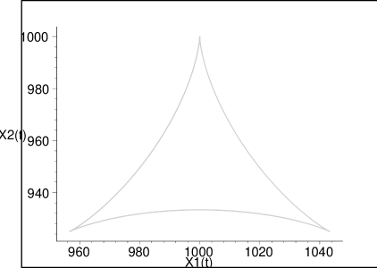
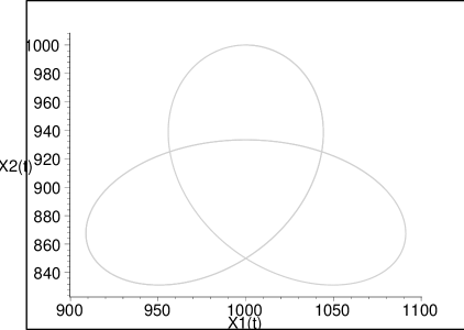
II.
In this case two circular movements superpose. It leads to the appearance of loops, sudden changing of direction and other complicated trajectories. Several examples are presented on Figures 2 and 3.
III.
Here the movement is also almost circular, but its radius is
IV. the resonance case. The motion is spiral, moreover, within some time the vortex can approach to the point with the coordinates and then move away. One of the possible situation is presented on Figure 4. Stress that this case hardly can be realized in the atmosphere, as the value of changes with the latitude.
In the situations presented on the Figures
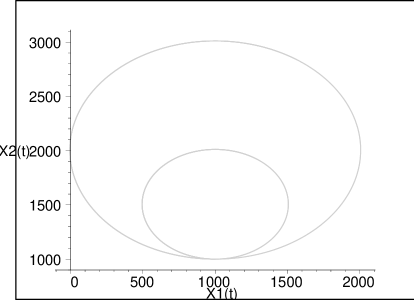
Figure 1. A circular trajectory. Here (the minor circle) (the larger circle).
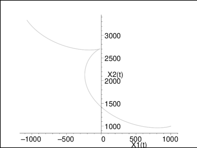
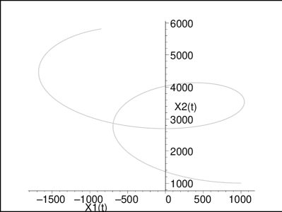
Figures 2 and 3. A slowly rotating typhoon (loops and change of direction). Here (Fig.2) (Fig.3).
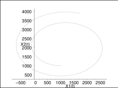
Figure 4. Resonance case. Here
Figures 5 and 6. A ”making time” typhoon. The examples of exotic trajectories are presented. Here (Fig.5), (Fig.6).
Let us stress, that as usual, except several cases, in the real atmosphere the typhoon doesn’t pass throughout all the trajectory before its decay, and one can speak about a part of this trajectory. Moreover, because the eye is not exactly in the equilibrium point, its trajectory oscillates near the trajectory presented in the picture.
Note that the rather usual behavior of intense typhoons is the motion first along the almost circular trajectory, becoming more curved as rises, and then along the almost strait trajectory. This can be explained as follows: if we are in the situation of quickly rotating typhoon (case I according to the classification of this section,), then firstly the difference is rather large, and the decisive influence to the value of radius of trajectory has the Coriolis parameter itself (see formula (4.1)). However, as the Coriolis parameter raises, this difference becomes small, it implies the augmentation of radius, thus the trajectory can look like a strait line. We can give examples of such typhoons: Isaac, category: 4 , 21 Sep – 01 Oct, 2000, Atlantic; Mitag, category: 5, 26 Feb – 08 Mar, 2002, Western Pacific; Pongsona, category: 4, 2–11 Dec, 2002, Western Pacific; Fabian, category: 4, 27 Aug – 08 Sep, 2003, Atlantic. (Recall that the number of category increases with the intensity of typhoon, the greatest is 5th, where the maximum wind amount to and higher.)
Typhoons, which trajectories loop, as usual (but not necessarily), are not very intense. Examples are the following: Fung Wong, category: 1, 20–27 July, 2002, Western Pacific; Tropical depression 28W, 18 –24 July, 2001, Western Pacific; Kyle, category: 1, 30 Sep – 12 Oct, 2002, Atlantic (however, Danas, category: 4, 3–12 Sep, 2001, Atlantic; Saomai, category: 5, 3–16 Sep, 2000,Western Pacific). They can be related to class II, on Figs.2 and 3 such trajectory is obtained for ”slow” typhoons, but one can get trajectories with loops and for intense typhoons, too.
At last it is possible that the typhoon passes to other equilibrium. It is known that that it can decay and regenerate several times. However it signifies that the trajectory of its motion modifies according to a new regime. Thus, as a rough approximation, the trajectory will be glued from several standard parts.
Forecasting possibilities
As we can see, in the frame of our model the trajectory behavior completely depends on initial data. The finding of correct initial data is a separate difficult problem, not only mathematical, but physical and statistical. The procedure of self-adapting (described in the introduction) may be of great use for this purpose.
Acknowledgements
The work was partially supported by the Russian Foundation of Basic Research Award no.03-02-16263 and the Leading Scientific Schools Project no.1464.2003.1.
The author is grateful to H.Fujita Yashima for attracting the attention to the subject and discussion, and to E.R.Rozendorn and V.A.Gordin for the interest to the work and useful commentaries.
References
-
[1]
http://weather.unisys.com/hurricane/index.html
http://www.aoml.noaa.gov/hrd/tcfaq/tcfaqHED.html
http://typhoon.atmos.colostate.edu/ - [2] Anthes, R.A.(1982) Tropical cyclones, Boston.
- [3] Hain, A.P. (1984) The mathematical modelling of tropical cyclones, Gidrometeoizdat, Leningrad, 247 p. (in Russian).
- [4] Kochin, N.E. (1922)A theoretical model of travelling cyclone in: Kochin N.E. Selected works, Vol.1, Moscow-Leningrad, Publication of the Academy of Science of URSS, 1949, pp.33–67.
- [5] Lord Rayleigh (1919). The travelling cyclone, Phylosophical Magazine, s.6, v.38, p.420.
- [6] Sir Napier Show (1918). The travel of circular depressions and tornadoes, Meteorologocal Office, Geophisical memoirs, N12.
- [7] Fridman A.A.(1921) An idea of rotating fluid in atmospherical motions, Meteorologicheskii vestnik, v.31, p.69. (in Russian)
- [8] Purganskiy, V.S. (1967)A method of computation of the trajectory of convective vortices of great intencivity, Trudy CAO (Publications of the Central aerologic observatory), issue 75, pp.84–96.(in Russian)
- [9] Kuo, H.L.(1963) Motion of vortices and circulating cylinder in shear flow with friction, J.Atm.Sci., v.26, N3, pp.390–398.
- [10] Shuleikin, V.V. (1973)On a computation of trajectory of tropical hurricanes, Izvestia of the Academy of Sciences of URSS, Physics of atmosphere and ocean, v.9, N 12, pp.1227–1238. (in Russian)
- [11] Jones, R.W. (1977) Vortex motion in a tropical cyclone model, J.Atm.Sci., v.34, N 10, pp.1518–1527.
- [12] Nesterova, A.V., Nesterov A.V. (1980)On a new model of a deplacement of tropocal cyclone, in book: Typhoon-78, Gidrometeoizdat, Leningrad, pp.202–213.
- [13] Khokhlova, A.V. (1984)Taking into account of parameters of the tropical cyclone in a semi-empirical model of its deplacement, Meteorology and Hydrology, N 10, pp.53–62.
- [14] Rostkova, T.B., Ordanovich, A.E. (1980)Applying of the method of self-adapting model to the study of the movement of tropical cyclone, Meteorology and Hydrology, N6, pp.49–56.
- [15] Rostkova, T.B., Ordanovich, A.E. (1982) The method of self-adapting model in application to problems of a determination of trajectory of tropical typhoon, In book: Certain problems of control dynamics of solid body, Moscow, Moscow State University Publishing.
- [16] Rostkova, T.B., Ordanovich, A.E. (1985) A forecasting of the trajectory of tropical cyclone according to the self-adapting model method, Meteorology and Hydrology, N1, pp.15–20.
- [17] Rostkova, T.B., Ordanovich, A.E. (1985) On a sensibility of the trajectory of tropical cyclone to certain parameters or equations describing its motion, Meteorology and Hydrology, N4, pp.110–114.
- [18] Dobryshman, E.M. (1994), Certain statistical characteristics and pecular features of typhoons, Meteorology and hydrology, no.11, pp.83 – 99.
- [19] Dobryshman, E.M. (1995), A nonstationary model of the typhoon eye, Meteorology and hydrology, no.12, pp.5 – 18.
- [20] Bulatov, V.V., Vladimirov, Yu.V., Danilov, V.G., Dobrokhotov, S.Yu.(1994)Calculations of hurricane trajectory on the basis of V. P. Maslov hypothesis. Dokl. Akad. Nauk, Ross. Akad. Nauk 338, No.1, pp.102–105.
- [21] Bulatov, V.V.; Vladimirov, Yu.V.; Danilov, V.G.; Dobrokhotov, S.Yu.(1994)On motion of the point algebraic singularity for two-dimensional nonlinear equations of hydrodynamics Math. Notes 55, No.3, pp.243–250; translation from Mat. Zametki 55, No.3, pp.11–20.
- [22] Bulatov, V.V.; Vladimirov, Yu.V.; Danilov, V.G.; Dobrokhotov, S.Yu.(1995) Propagation of point algebraic singularity for nonlinear equations of hydrodynamics and modelling of middle-scale vortices in nongomogenious atmosphere on the base of V.P.Maslov’ hypotesis. Preprint N 552, Institute of the mechanics problems RAS.
- [23] Dobrokhotov, S.Yu.(1999) Hugoniot-Maslov chains for solitary vortices of the shallow water equations. I: Derivation of the chains for the case of variable Coriolis forces and reduction to the Hill equation, Russ. J. Math. Phys. 6, No.2, pp.137–173.
- [24] Maslov V.P.(1980), Three algebras, corresponding to nonsmooth solutions to systems of quasilinear equations, Uspekhi Matematicheskih nauk, v.35, v.2(212), pp.252–253.
- [25] Ravindran, R, Prasard, P. (1990) A new theory of shock dynamics, Part I(II), Applied Mathematics Letters,(3), no.2(3), pp.107–109.
- [26] Gruza, G.V., Gres’ko, P.D. Statistical method of prognosis of tropical cyclons mouvement in Atlantic, Leningrad, Gidrometeoizdat, 1977, 134 p. (in Russian).
- [27] Moisseev, S.S., Oganian, K.R., Rutkevich, P.G., Tur, A.V. Influence of phase transitions of moisture to processes of generation of large-scale vortices in the stratufied turbulent atmosphere, Proceedings of the conference ”Problems of stratified flows”, Salaspils, 1988, Vol.2, pp.37–41.
- [28] Alishaev D.M.(1980), On dynamics of two-dimensional baroclinic atmosphere Izv.Acad.Nauk, Fiz.Atmos.Oceana,16, N 2, pp.99–107.
- [29] Intense atmospheric vortices. Proceedings of the Joint Simposium (IUTAM/IUGC) held at Reading (United Kingdom) July 14-17, 1981. Edited by L.Begtsson and J.Lighthill.
- [30] Obukhov A.M.(1949), On the geostrophical wind Izv.Acad.Nauk (Izvestiya of Academie of Science of URSS), Ser. Geography and Geophysics,XIII, pp.281–306.
- [31] Landau, L.D.; Lifshits, E.M.(1987), Fluid mechanics. 2nd ed. Volume 6 of Course of Theoretical Physics. Transl. from the Russian by J. B. Sykes and W. H. Reid. (English) Oxford etc.: Pergamon Press. XIII, 539 p.
- [32] O.S.Rozanova (2002): On classes of globally smooth solutions to the Euler equations in several dimensions. LANL e-print math.AP/0203230.
- [33] O.S.Rozanova (2003):On classes of globally smooth solutions to the Euler equations in several dimensions. In: Hyperbolic problems:Theory, Numerics, Applications. Proceedings of the Ninth International Conference on Hyperbolic problems held in CalTech, Pasadena, March 25–29, 2002. Springer. pp.861–871.
- [34] O.S.Rozanova(2003), Application of integral functionals to the study of the properties of solutions to the Euler equations on riemannian manifolds, J.Math.Sci. 117(5), pp.4551–4584.
- [35] Gray W.M.(1968)Global view of the origin of tropical disturbances and storms, Mon.Weath.Rev., v.96, pp.669–700.