Two-dimensional trapping of dipolar molecules in time-varying electric fields

Abstract

Simultaneous two-dimensional trapping of neutral dipolar molecules in low- and high-field seeking states is analyzed. A trapping potential of the order of 20 mK can be produced for molecules like ND₃ with time-dependent electric fields. The analysis is in agreement with an experiment where slow molecules with longitudinal velocities of the order of 20 m/s are guided between four 50 cm long rods driven by an alternating electric potential at a frequency of a few kHz.

Cold molecules offer new perspectives, e.g. for high precision measurements  Hinds and collisional physics studies  Balakrishnan . Pioneering work on cold molecules has been done using cryogenic buffer gas cooling Weinstein . Another promising technique for the production of cold molecules is based on the interaction of dipolar molecules with inhomogeneous electric fields. For example, low-field seeking molecules (LFS) have been slowed down in suitably tailored time-varying electric fields  MeyerDecel and have been trapped in inhomogeneous electrostatic fields  MeyerRing ; MeyerTrap . Furthermore, efficient filtering Bookcont of slow LFS from an effusive thermal source using a bent electrostatic quadrupole guide has been demonstrated Rangwala .

Compared to LFS, the manipulation of high-field seeking molecules (HFS) is much more difficult. This is mainly due to the fact that electrostatic maxima are not allowed in free space, and hence, HFS are quickly lost on the electrodes. Nevertheless, guiding of HFS in Keppler orbits Loesch and deceleration as well as acceleration of HFS MeyerAG is possible. Despite this progress in manipulating dipolar molecules, all techniques realized so far are suited only for either LFS or HFS, not both simultaneously. However, in future experiments with trapped samples of cold molecules, collisions or the interaction with light fields are likely to change HFS into LFS and vice versa. Therefore, a technique to trap both species simultaneously is vital. In this Letter, we investigate both theoretically and experimentally a new technique, which can trap both HFS and LFS. In particular, we report on the first experimental demonstration of two-dimensional trapping of slow ND₃ molecules from an effusive source in a bent four-wire guide driven by an alternating electric field.

Trapping neutral particles in oscillating electric fields works as follows Shimizu92 . The force on a molecule in an electric field, $E$, is given by $\vec{F}=-\vec{\nabla}W(E)$, with $W(E)$ the Stark energy of the molecule. Polar molecules like ND₃ and H₂CO predominantly experience a linear Stark shift, $W=s\,E$, where $s$ is the slope of the Stark shift. Other molecules, however, and atoms usually experience a quadratic Stark effect, $W=-\frac{1}{2}\alpha E^{2}$, with the polarizability $\alpha$.

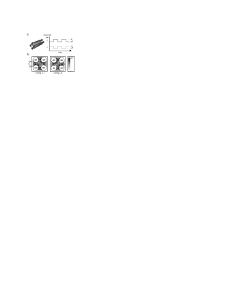
Figure 1: Schematic of the four-wire setup for typical operating voltages of $\pm 5\,$kV, where $E_{0}=35\,$kV/cm and $\beta=2.3\times 10^{3}\,$kV/cm³. The voltages on a pair of opposite electrodes are switched as shown in (a) in order to produce a time-varying field that alternates between configurations 1) and 2) shown in (b) with a repetition rate in the kHz range. The radius $r_{max}$ used in simulations is indicated by the dashed circles.

The inhomogeneous electric fields required for trapping can be realized in many different ways. Our trapping configuration is sketched in Fig. 1. It consists of 4 parallel rods with voltages as indicated. The field is rapidly switched between two dipole-like configurations with angular frequency $\omega$. Close to the center, the field can be expanded harmonically,

$$E=E_{0}+H(t)\beta(x^{2}-y^{2}),$$ (1)

where $E_{0}$ is the field in the center and $\beta$ is (half) the curvature of the field. The step function $H(t)=1$ if $nT<t<(n+\frac{1}{2})T$ and $H(t)=-1$ otherwise, with $T=2\pi/\omega$ the period of the driving field and $n$ an integer.

Independent of the slope and the sign of the Stark shift, the saddle-like dipole potential derived from Eq.(1) confines the particle in one direction and repels it in the perpendicular direction, depending on time. Therefore, the time average of the force is small at every position, and identical to zero for a linear Stark shift. However, the particle performs a micromotion which is locked to the external driving field so that the time-averaged force does not cancel and the particle experiences a net attractive force towards the center. This conclusion is independent from the exact form of H(t). Therefore, a sinusoidal change between two configurations would also work. However, instantaneous switching is more convenient to realize in the laboratory.

It is not difficult to solve the equation of motion for molecules in this dynamic field. As the x and y degrees of freedom separate, the equation of motion is reduced to one dimension. It reads $\ddot{x}=-H(t)\Omega^{2}x$, where we have introduced $\Omega^{2}=2s\beta/m$ for a linear Stark shift and $\Omega^{2}=2\alpha E_{0}\beta/m$ for a quadratic Stark shift of a particle with mass $m$. Following Morinaga94 , we search for orbits of the form $(x(t),\dot{x}(t))=U(t)(x(0),\dot{x}(0))$ with $U(nT+t)=U(t)[U(T)]^{n}$. Periodic solutions have the form $U(T)=U_{2}(T/2)\,U_{1}(T/2)$, with $(U_{1}(t),U_{2}(t))=\left(\!\left(\!\begin{array}[]{cc}\cosh(t\Omega)&\frac{1}{\Omega}\sinh(t\Omega)\\ \Omega\sinh(t\Omega)&\cosh(t\Omega)\end{array}\!\right)\!,\left(\!\begin{array}[]{cc}\cos(t\Omega)&\frac{1}{\Omega}\sin(t\Omega)\\ -\Omega\sin(t\Omega)&\cos(t\Omega)\end{array}\!\right)\!\right)\\$the evolution operators for the first and the second half cycle. From this, the main stable region can be found for $|\Omega T|\leq 3.75$. Narrow higher-order stable regions also exist but will further be neglected. Hence there exists a sharp drive-frequency threshold for every Stark shift, above which trapping is possible, irrespective of the sign of the Stark shift and independent of the initial conditions.

Note that the finite extension of our trap, $|x|\leq x_{max}$, limits the trap depth. This can be estimated by averaging over the micromotion, which is assumed to be smaller and faster than the macromotion. This results in a trap depth $m\pi^{2}x_{\rm{max}}^{2}\Omega^{4}/(24\omega^{2})$, typically of the order of 10 mK  Ghosh . For a more realistic estimate, a detailed analysis is made below.

It is interesting to compare molecule trapping with ion trapping in a Paul trap Ghosh . An ion experiences the Coulomb force $\vec{F}_{\rm C}$, which has zero divergence, $\vec{\nabla}\cdot\vec{F}_{\rm C}=0$. As a consequence, the the magnitude of the force is the same for positive and negative ions. For molecules with a linear Stark shift and in the harmonic approximation, $\vec{\nabla}\cdot\vec{F}=0$, and there is an accidental correspondence with the equations of motion of an ion in a Paul trap. It should nevertheless be emphasized that trapping neutral molecules differs from ion trapping in many ways. First, whereas ions are monopolar particles which can be trapped in an oscillating quadrupole field, neutrals have permanent or induced dipoles which can be trapped in an oscillating dipole field. Second, in contrast to ions, the force on a molecule in an electric field depends dramatically on the internal state of the molecule. Third, as is obvious from Fig. 1, the harmonic approximation is only valid in a small region around the center. In contrast to ions, which have vanishingly little kinetic energy compared to the $10^{5}\,$K trap depth, the temperature of the molecules is likely to be comparable to the trap depth. Hence, molecules explore the full volume of the shallow trap, including the outer regions. These outer regions are of paramount importance in our experiment. It is here that the harmonic approximation breaks down. The molecule-field interaction even allows $\vec{\nabla}\cdot\vec{F}\not=0$. This leads to different behavior for HFS and LFS away from the center, where the time-average of the force in configurations 1) and 2) is not zero. In particular, the regions near the electrodes are net repulsive for LFS and net attractive for HFS.

To take all these effects into account, we have performed a two-dimensional Monte Carlo simulation. In the simulation, point-like particles are injected on-axis in a random phase of the driving field. The input velocities $v_{x}$ and $v_{y}$ are varied. The particles are propagated under the influence of the periodically poled Stark force for 10 ms, a typical time in the experiment. They are considered lost if they leave a radius $r_{max}=1.25\,$mm. The amount of trapped trajectories can be expressed as an area $A$ in the two-dimensional $v_{x}v_{y}$-velocity space quadrant. $A$ is a good measure for the flux, if the guidable velocities are equally present in the source. Results for four different molecular states of ND₃ exhibiting linear Stark shifts with a slope, $s$, of $\pm$ 0.6 cm^-1/(100 $\frac{kV}{cm}$) and $\pm$ 1.2 cm^-1/(100 $\frac{kV}{cm}$) are plotted in Fig. 2. For a molecular state with a Stark shift of 1.2 cm^-1/(100 $\frac{kV}{cm}$) and at 9 kHz for our experimental parameters, the occupied $v_{x}v_{y}$-space has almost a quarter-disc shape, with which a trap depth of approximately 20 mK can be associated.

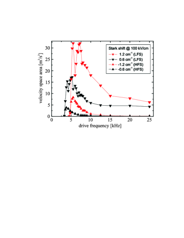
Figure 2: Area of guided molecules in transverse-velocity space obtained from a two-dimensional Monte-Carlo simulation. Curves for LFS ($\blacktriangledown,{\color[rgb]{1,0,0}\blacktriangledown}$) and HFS ($\blacktriangle,{\color[rgb]{1,0,0}\blacktriangle}$) ND₃ molecules with the given Stark shifts are displayed.

As expected from the analytic analysis, there is a sharp turn-on frequency above which guiding is possible both for LFS and HFS. For increasing frequencies, the area $A$ reaches a maximum before decreasing again for higher frequencies. Note that the maximum of $A$ is approximately four times larger for LFS than for HFS, indicating that LFS can be guided more efficiently. This is due to the anharmonicity of the trapping potential away from the center, where stable trajectories exist for LFS with comparatively high initial velocities. This effect also causes the substructure in the LFS curves in Fig. 2. For even higher frequencies, the amplitude of the micromotion becomes very small and the force on the molecules approaches the time-average of the force in configurations 1) and 2). This time-averaged force is small near the center but substantial and repulsive near the electrodes. Stable orbits therefore exist in the high-frequency limit for LFS. The stable orbits occupy disjunct areas in velocity space, of which the area, $A$, saturates. The notion of a trap depth becomes difficult in this limit. The behavior of HFS, however, is completely different: With the disappearing micromotion, there are no stable trajectories and $A$ vanishes in the limit of high drive frequency.

Obviously, the motion in the full anharmonic potential can be very complicated. In fact, we have found numerical evidence for chaotic motion for some initial conditions. But despite of the complicated dynamics, LFS and HFS are simultaneously trapped and there is a broad overlap between the trapping regions for different Stark shifts at the same frequencies, as evident from Fig. 2.

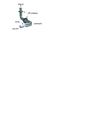
Figure 3: Schematic of the experimental setup. ND₃ molecules emerging from the nozzle are injected into the guide. The slowest molecules are kept within the guide and after passing two differential pumping stages they enter a UHV chamber where they are detected with a mass spectrometer. The fast molecules are pumped away.

Our experimental demonstration of AC guiding uses an effusive source of thermal polar ND₃ molecules, see the setup shown in Fig. 3 Rangwala . The double-bent guide consists of four wires which pass through two vacuum chambers with two differential pumping sections before ending in a UHV detection chamber. The guide has a length of 500 mm and is made of 2 mm diameter stainless steel rods, with a 1 mm gap between neighboring rods. The radii of curvature of the two bends are 25 mm and the rods are built around the 0.8 mm inner diameter ceramic nozzle, constituting the effusive source. Typical operation pressures in the nozzle are around 0.05 mbar in order to maintain molecular-flow conditions. Most of the molecules are not guided and escape into the first vacuum chamber, where an operational pressure of a few times $10^{-7}\,$ mbar is maintained. In the detection chamber, where a pressure below $10^{-10}\,$ mbar is achieved, the guided molecules are detected with an efficiency of about $10^{-4}$ counts/molecule by a quadrupole mass spectrometer (QMS)[Hiden Analytical, HAL 301/3F] with a pulse-counting channeltron. The pulses from the channeltron are processed in a multi-channel scaler. The ionization volume of the QMS begins 22 mm behind the guide. To protect the QMS from the high electric fields, a metal shield with a 5 mm diameter hole is placed 1 cm behind the exit of the guide. The time-varying electric fields are generated by switching high voltages with fast push-pull switches. Switching frequencies are typically in the range of a few kHz. In each phase of the alternating field, opposite rods carry voltages of up to $\pm\,7\,$kV. Due to the inversion splitting of the vibrational ground state, ND₃ shows in good approximation a linear Stark shift in the relevant electric field range (0-100) kV/cm  Schawlow .

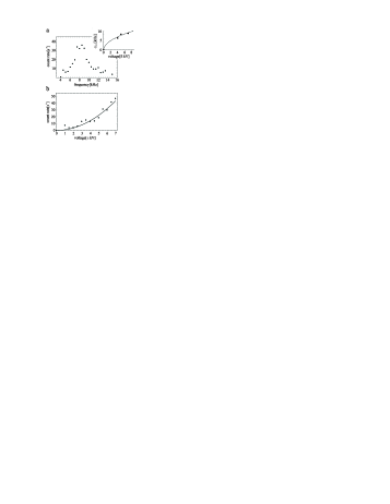
Figure 4: (a) Molecular flux as a function of the applied frequency for rod voltages of $\pm 5\,$kV. The graph in the inset shows the frequency of maximum flux, $\omega_{0}$, as a function of the applied voltage. The dashed line indicates the $\omega_{0}\propto\sqrt{V}$ dependence. (b) Flux as a function of the applied voltage. For each voltage, the frequency is adjusted for maximum flux according to (a). The line is a quadratic fit.

For detecting ND₃ molecules the QMS is set to mass 20. The influence of other gases at this mass is negligible. The QMS does not provide state-selective detection, which is very difficult to achieve if one considers the variety of molecular states involved in a thermal (room-temperature) ensemble. Our simulation, however, shows that the detection of HFS is suppressed, because under the influence of the high electric fields most of the HFS turn around at the exit of the guide, moving backwards on its outside, or they are reflected back into the guide.

To discriminate the guided molecules from background gas and dark counts, the alternating electric field is periodically applied for 200 ms followed by a 200 ms where no field is applied. This on-off sequence is repeated about 40000 times to obtain a good signal-to-noise ratio. From the instant when the alternating field is switched on, the molecules can propagate along the guide and the signal rises. After about 25 ms, the signal has reached 50% of the maximum increase, corresponding to velocities around 20 m/s or about 0.5 K. When the alternating field is switched off the flux instantaneously falls off. The flux of guided molecules is determined by subtracting the background count rate from that during the last 50 ms of the 200 ms-long interval where the field is applied. The same measurement without injecting gas yields no signal.

We now investigate the frequency dependence of the system. For electrode voltages of $\pm$5 kV, the switching frequency is varied between (4-15) kHz, and the flux of guided molecules is recorded in frequency steps of 500 Hz. The experimental data in Fig. 4a show that the signal amplitude reaches a pronounced maximum at a frequency of $\approx$8 kHz. No discernible signal is observed for frequencies below 4 kHz. This behavior can be understood from the simple analytic theory above, acknowledging the thermal ensemble of molecular states. For every molecular state there exists a cut-off frequency corresponding to the associated Stark shift below which no guiding is possible. This frequency increases with the Stark shift. For example, the cut-off frequencies for molecules with Stark shifts of 0.6 cm^-1 and 1.2 cm^-1 at an electric field strength of 100 kV/cm in our guide are 3.3 kHz and 4.7 kHz, respectively. For small frequencies stable trajectories exist only for molecules with small Stark shifts. These molecules are unlikely to be guided as the potential depth is too small compared to their kinetic energy. Higher frequencies allow stable trajectories for molecules with higher Stark shifts and so the number of guidable states increases. Furthermore the guiding efficiency for molecules with higher Stark shifts is much higher. Both effects cause the rise in the count rate for frequencies below 8 kHz. For higher frequencies the count rate decreases because the guided flux for every molecular state depends on the depth of the potential which drops off with $\omega^{-2}$.

Our conclusions are supported by two additional measurements. First, the dependence between the applied voltage and the frequency $\omega_{0}$ for which optimum guiding exists is analyzed. In the harmonic approximation, the stable region is given by $|\Omega T|\leq 3.75$ with $\Omega\propto\sqrt{\beta}$. As the curvature $\beta$ scales linearly with the applied voltage $V$, we obtain $\omega_{0}\propto\sqrt{V}$. Experimental data are shown together with the expected square root dependence in the inset of Fig. 4a. Unfortunately, the measurements cover only a small voltage interval, because for small voltages no guiding signal could be obtained, whereas sparks occurred for higher voltages. Nevertheless, the measured data agree with the calculated scaling. This allows one to choose the optimum switching frequency for a given voltage. In a second measurement, the flux is measured as a function of the applied voltage, using the optimum frequency for each voltage. The experimental data in Fig. 4b show a quadratic rise in flux with increasing voltage. This is expected for ND₃, where most states have a linear Stark shift Rangwala .

To summarize, two-dimensional trapping of neutral molecules with alternating electric fields is demonstrated experimentally. Our result proves that molecules with transverse and longitudinal temperatures of 20 mK and 0.5 K, respectively, can be filtered out of a room temperature effusive source efficiently. Our simulation shows that both HFS and LFS are guided, whereas the low-field seekers are guided and detected with a higher efficiency. The guiding efficiency for both classes will further increase if the injected molecules are precooled with cryogenic methods. An important aspect of our guide is that it is suited to trap laser-cooled atoms as well Shimizu92 . Two-dimensional trapping of both atoms and molecules should therefore be possible. Finally, an extension of our technique to trap sufficiently slow molecules in three dimensions Shimizu92 should be feasible.

References

- (1) J.J. Hudson, B.E. Sauer, M.R. Tarbutt, and E.A. Hinds, Phys. Rev. Lett. 89, 023003 (2002).
- (2) N. Balakrishnan, A. Dalgarno, Chem. Phys. Lett. 341, 652-656 (2001).
- (3) J.D. Weinstein et al., Nature (London) 395, 148 (1998).
- (4) H.L. Bethlem, G. Berden, and G. Meijer, Phys. Rev. Lett. 83, 1558 (1999).
- (5) F.M.H. Crompvoets, H.L. Bethlem, R.T. Jongma, and G. Meijer, Nature 411, 174 (2001).
- (6) H.L. Bethlem, G. Berden, F.M.H. Crompvoets, R.T. Jongma, A.J.A. van Roij, and G. Meijer, Nature 406, 491 (2000).
- (7) P.W.H. Pinkse, T. Junglen, T. Rieger, S.A. Rangwala, and G. Rempe, Interactions in Ultracold Gases, edited by M. Weidemüller and C. Zimmermann, (Wiley-VCH, Weinheim, 2003).
- (8) S.A. Rangwala, T. Junglen, T. Rieger, P.W.H. Pinkse, and G. Rempe, Phys. Rev. A 67, 043406 (2003).
- (9) H.J. Loesch and B. Scheel, Phys. Rev. Lett. 85, 2709-2712, (2000).
- (10) H.L. Bethlem, A.J.A. van Roij, R.T. Jongma, and G. Meijer, Phys. Rev. Lett. 88, 133003 (2002).
- (11) F. Shimizu and M. Morinaga, Jpn. J. Appl. Phys. 31, L1721 (1992).
- (12) D. Auerbach, E.E.A. Bromberg, and L. Wharton, J. Chem. Phys. 45, 2160 (1966).
- (13) M. Morinaga and F. Shimizu, Laser Physics 4, No. 2, 412 (1994).
- (14) P.K. Ghosh, Ion Traps, (Clarendon Press, Oxford, 1995).
- (15) C.H. Townes and A.L. Schawlow, Microwave Spectroscopy, (Dover Publications, Inc., New York, 1975).